Review

A Compendious Review on the Determination of Fundamental Site Period: Methods and Importance

Ingram School of Engineering, Texas State University, San Marcos, TX 78666, USA
Geotechnics 2023, 3(4), 1309-1323; https://doi.org/10.3390/geotechnics3040071
Submission received: 9 October 2023 / Revised: 28 November 2023 / Accepted: 30 November 2023 / Published: 4 December 2023
(This article belongs to the Special Issue Recent Advances in Geotechnical Engineering (2nd Edition))

Abstract

:
It is now well-known that ground motion characteristics can be influenced significantly by local site characteristics. In general, soil characteristics were classified by considering the time-average velocity down to 30 m (Vs30). However, recent studies have showed that the fundamental site period is a better proxy than Vs30, or the most complementary parameter to Vs30, for this purpose. Recent earthquakes have also revealed that the largest amplifications occur at the fundamental site period and cause heavy damage or the collapse of structures when they have similar vibrational characteristics with the site’s fundamental period, i.e., resonance. Therefore, many studies in the literature have been performed to determine the fundamental periods of layered soil profiles using different analytical, approximate, and data-driven methods. However, there is a requirement to evaluate these methods by following a systematic procedure. Hence, the reader will receive a comprehensive review of the available procedures for determining the site’s fundamental period of layered soil profiles and their applications at different scales, along with an exploration of current research gaps.

1. Introduction

It is now widely recognized that soil characteristics, particularly those of near-surface soil deposits, have a substantial effect on structural performance during intense strong ground motion [1]. Shallow soil deposits can amplify the effects of ground motion, such as acceleration on the surface, due to the wave impedance of relatively soft soils [2,3,4,5]. During earthquakes, structures experience the largest amplification when their structural periods match with the site’s fundamental period, resulting in resonance [6,7,8]. Therefore, mid- [3,9] and/or high-rise [10,11,12] structures resting on soft soils and low-rise structures resting on stiff soils [13] have higher vulnerability. Even low-rise buildings were observed to collapse during the 1943 and 1967 earthquakes in Adapazarı, Türkiye, where the fundamental periods were approximately 0.3 s [13]. This underscores the critical role of resonance in seismic vulnerability, emphasizing the need for a thorough understanding of soil-structure interaction to mitigate risks associated with different soil conditions.
In addition, the assessment of soil classification and local site effects has traditionally relied predominantly on only Vs30 [14]. However, it has been shown that the fundamental site period (T0) serves as a superior standalone proxy compared to Vs30 or, at the very least, the most effective complementary proxy toVs30 [15,16,17,18]. Notably, classifications based on the fundamental period have been shown to yield lower errors than conventional classifications solely based onVs30 [19,20,21,22].
The principal reason for the higher error associated with Vs30-based classification lies in the fact that Vs30 represents only near-surface stiffness. In contrast, the fundamental site period provides a more comprehensive representation, encapsulating both the stiffness and depth characteristics of the entire soil column [23]. This nuanced consideration allows for a more accurate and nuanced assessment of soil properties and seismic site conditions, emphasizing the importance of incorporating fundamental period-based analyses in geotechnical studies.
Due to the above-mentioned advantages, researchers have endeavored to enhance the precision of determining the fundamental site period through the development of analytical, numerical, data-driven methods, and artificial intelligence techniques. Several studies have delved into the effectiveness of these analyses [24,25,26,27,28,29,30]. While some studies indicate that one-dimensional (1D) ground response analysis (GRAs) falls short in capturing intricate soil characteristics [28], others report that 1D GRAs have reasonably good correlations with downhole array data [24,26,27,29,30]. These contrasting results underscore the complexity of soil-structure interactions and the diverse methods employed in their analysis.
Recognizing the pivotal role of fundamental site periods and the nuanced capabilities and limitations of 1D GRAs, this study offers a comprehensive state-of-the-art review of existing methodologies for calculating T0. This review includes analytical, numerical, data-driven, and artificial intelligence techniques, providing a systematic evaluation of the various approaches.
By shedding light on critical aspects of the topic, this study serves as a valuable resource for academia and industry professionals. The insights garnered from this review are poised to benefit researchers, engineers, and practitioners seeking a deeper understanding of the methodologies employed in determining fundamental site periods. This synthesis of methodologies and findings contributes to the ongoing discourse in seismic studies, facilitating informed decision-making and advancements in seismic risk assessment, and mitigation strategies.
The data for this study were obtained through an extensive literature search conducted on reputable databases, including Google Scholar, Scopus, and ScienceDirect. The search was executed using keywords such as site fundamental period, fundamental site period, site fundamental frequency, and fundamental site frequency. To ensure relevance and specificity of the gathered information, an initial exclusion criterion was applied to filter out studies pertaining solely to the fundamental period of specific structures, such as reinforced concrete or steel. Subsequently, the focus was refined to include studies presenting novel methodologies for determining the fundamental site period. The selected studies form the basis for citation and analysis in this research, providing a robust foundation for the investigation of innovative approaches in the determination of fundamental site periods.

2. Use of the Site’s Fundamental Period

Even though soils are characterized by the Vs30 value in many codes, it is now well-known that T0 is a better proxy than Vs30 or one of the best self-standing parameters for this purpose [15,16,17,18]. Furthermore, Vs30 is insufficient to reflect the site effects in many regions [31,32]. Therefore, in addition to determining resonance cases [33], the fundamental site period has also been used for ground motion prediction equations (GMPEs) [19,34].
Alessandro et al. [35] employed T0 for response spectra prediction equations in Italy. The study concluded that flat-frequency-response, deep, and shallow profiles were captured easily by considering T0. In addition, T0-based classification was found to be quick and cost-effective compared to shear-wave velocity-based methods.
Hassani and Atkinson [16] evaluated a Vs30-based site-effect model [36] for possible application to sites in central and eastern North America. The study revealed that while there was an acceptable level of correlation between site effects and Vs30 for regions with low frequency, i.e., high period, this correlation decreased significantly for regions with high fundamental site frequencies. Hassani and Atkinson [17] evaluated the efficiency of T0 as a proxy to Vs30 in central and eastern North America, aiming to reduce Vs30-related errors and the associated random variability of GMPEs. The study obtained a 3% reduction in variability on average when T0 was employed as a proxy for Vs30. It was stated that a greater reduction could be achieved by replacing Vs30 with improved site characterization parameters such as T0. Later, Hassani and Atkinson [18] developed a regional site-effects model for central and eastern North America, where the residuals were determined based on T0 for a selected database from NGA-East. The study showed that the random variability of GMPEs can be reduced by an average of 10% when Vs30 is replaced with T0. Finally, Hassani and Atkinson [37] developed an empirical site-response model for central and eastern North America by evaluating residuals of observed ground motion amplitudes concerning those obtained by a selected GMPE. In the study, two alternatives for site effects were considered. In the first alternative, T0 was the main parameter, while Vs30 was the proxy. In the second alternative, the conventional order was preferred. The study showed that the use of T0 as the primary site parameter could remove most Vs30-dependent trends in the site terms, and derive a satisfactory single-parameter model. Furthermore, Vs30 was found to be an inefficient parameter for the studied region. Recently, Yazdi et al. [38] showed that incorporating T0 into NGA-West2 ground motion models could significantly lower uncertainties, by an average of 13%.
Kotha et al. [39] stated that the classification of soils considering T0 for GMPEs works well at first; however, it may be insufficient to distinguish sites with identical T0 ranges but different amplification levels.
Kwak and Seyhan [40] described a two-stage nonlinear site amplification model for Japan, considering Vs30 and T0. In this model, the total empirical site effects were regressed based on Vs30, and then a function was fitted to the residuals considering T0. The study found that the first term reduces errors at mid-to-long period ranges, while the second term further reduces errors.

3. Determination of the Site’s Fundamental Period

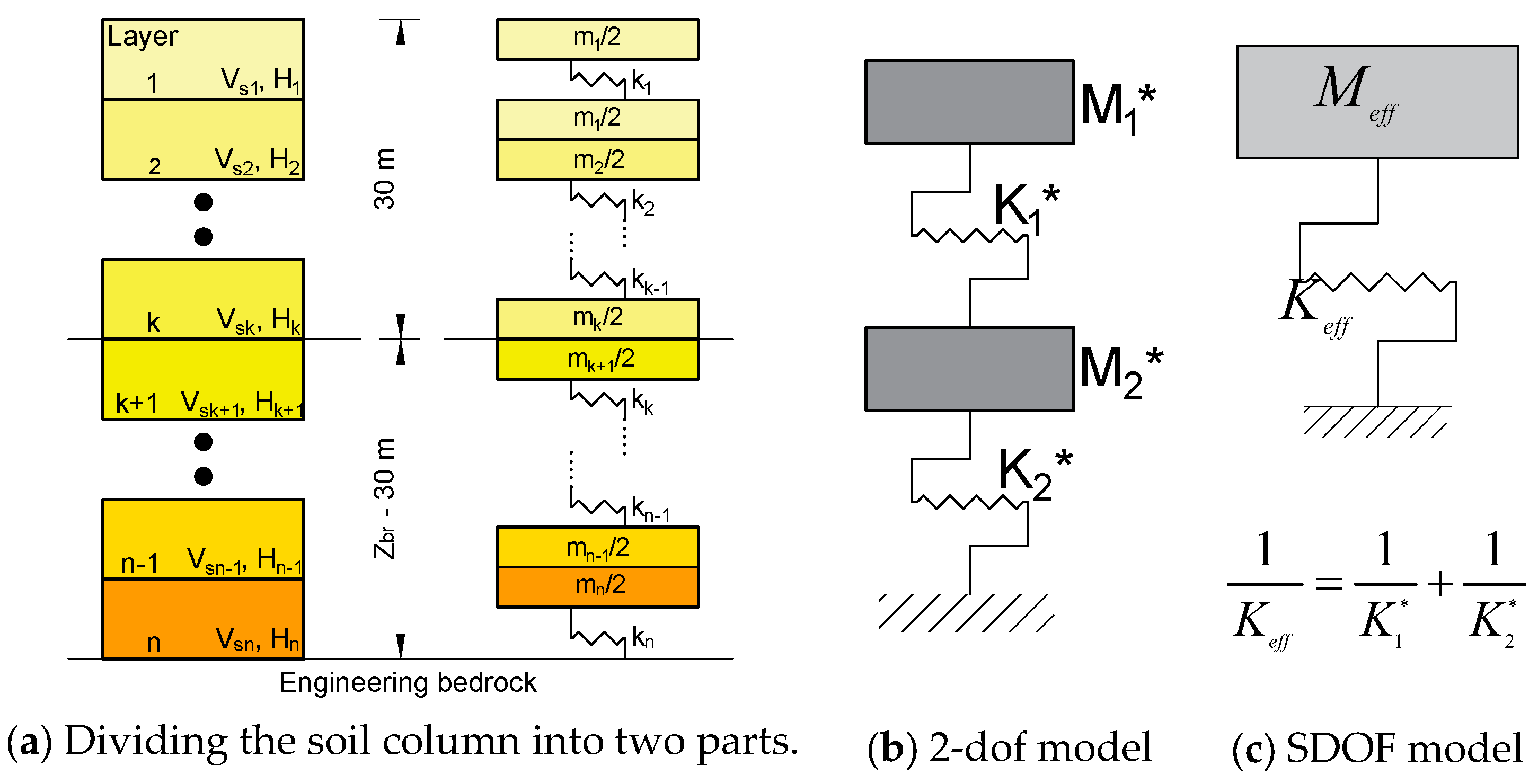
3.1. Analytical Methods

Early studies in the literature proposed analytical equations to calculate the site’s fundamental period, such as the linear shear modulus distribution method proposed by Ambraseys [41], Equation (1a), where the depth of the soil column is shown by H. The terms, K and V0, in the equation are given by Equations (1b) and (1c). In these equations, G0, GH, and ρ stand for the shear modulus at the top layer, shear modulus at the base of the layer, and density. The term α 1 is the first root of Equation (2), where Ji (i = 0, 1) and Yi (i = 0, 1) are the Bessel functions and Weber’s Bessel functions of order zero and one.
T = 4 π H K α 1 | 1 K 2 | V 0
K = G 0 / G H
V 0 = G 0 / ρ
J 0 ( α 1 ) Y 1 ( K α 1 ) J 1 ( K α 1 ) Y 0 ( α 1 ) = 0
Idriss and Seed [42] calculated the fundamental site period by considering the power-law distribution of the shear wave velocity, as given in Equation (3). In the equation, q1 is the first root of Jn(q1) = 0, where Jn( ) is the Bessel function of order n = (p − 1)/(2 − p).
T = 4 π H ( 2 p / 2 ) ( 2 ρ ) V 0 q 1
To simplify the problem, Madera [43] proposed a two-layer model. The method requires the calculation of the fundamental period of each layer (Ta and Tb) by Equation (4) and combining them considering Equation (5) to reach the final value (Tab). In the equations, ha and hb represent the heights of each layer. Later, an approximate solution to Madera’s method [42] was suggested by Hadjian [44].
T i = 4 h i V i ,       ( i = a ,   b )
tan ( π 2 T a T a b )   tan ( π 2 T b T a b ) = ρ b h b ρ a h a T a T b
The suggestion by Dobry et al. [45] to determine the fundamental site period is based on four times the travel time of the shear wave from bedrock to the ground surface, as shown in Equation (6). In the equation, i is the number of layers in the soil column. However, it was stated that this method overestimates the fundamental period by 20% [23]. Therefore, a correction factor was proposed by Motazedian et al. [46], as given in Equation (7). Later, Urzua et al. [47] showed that this method results in overestimation when the shear wave velocity increases with the depth of the soil column. Wang et al. [23] employed the simplified single-degree-of-freedom system method to improve Equation (6), resulting in Equation (8).
T i = 4 i = 1 n h i V i  
T i = 0.796 × ( 4 i = 1 n h i V i   ) 0.920
T i = π i = 1 n h i V i
Gazetas [48] also considered a linear shear wave velocity distribution through the depth of the soil column to obtain the fundamental site period, as seen in Equation (9). In this equation, η1 and μ1 are the first non-zero root of Equation (10) and the base-to-surface velocity ratio, respectively. The term a1 is a function of depth, travel time from surface to bedrock, and soil column height [23].
T = 4 H a 1 π ln μ 1 2 ( μ 1 1 ) η 1 2 + ( ln u ) 2
2 η 1 cos η 1 + ln ( μ 1 ) sin η 1 = 0
The Rayleigh method, which is considered one of the most convenient solutions for the studied problem, is based on equalizing the maximum kinetic and potential energies of the soil column system during its first mode of free vibration [49]. The solution is given by:
T = 2 π 0 H ρ X 2 d z 0 H ρ V ( d X d z ) 2 d z
where X(z) is the mode shape of the fundamental period at depth, z, ρ ( z ) = γ ( z ) / g , γ ( z ) is the unit weight of the soil at the same depth, and g is gravitational acceleration. Accordingly, the solution of Equation (11) requires computation of the fundamental modal shape of the soil column, which can be obtained through the equilibrium between inertial and elastic forces at depth z, as seen in Equation (12). The equation requires an iterative solution until the successive solutions, X(j) and X(j+1), are close enough.
X j + 1 ( z ) = 0 z [ ζ H ρ ( z ) X j ( z ) d z ] d z a ρ ( z a ) V 2 ( z a )
Due to the iterative nature of the Rayleigh method, Dobry et al. [45] proposed a simplified Rayleigh method that considers constant density of soil throughout the depth. These assumptions significantly simplified the solution, yielding fast convergence and high effectiveness, i.e., <3% relative error [48].
The Japanese seismic design code [50] considers the weighted value of a soil layer and employs the square root of the sum of the squares method to reach the fundamental site period, as shown in Equation (13), where the weight value of the soil layer is represented by the term 2 Hmi/hi, where H m i = H i 1 + H i / 2 . In the equation, h and H are the thickness and depth of the layer.
T = i = 1 n ( 4 h i V i ) 2 2 H m i h i

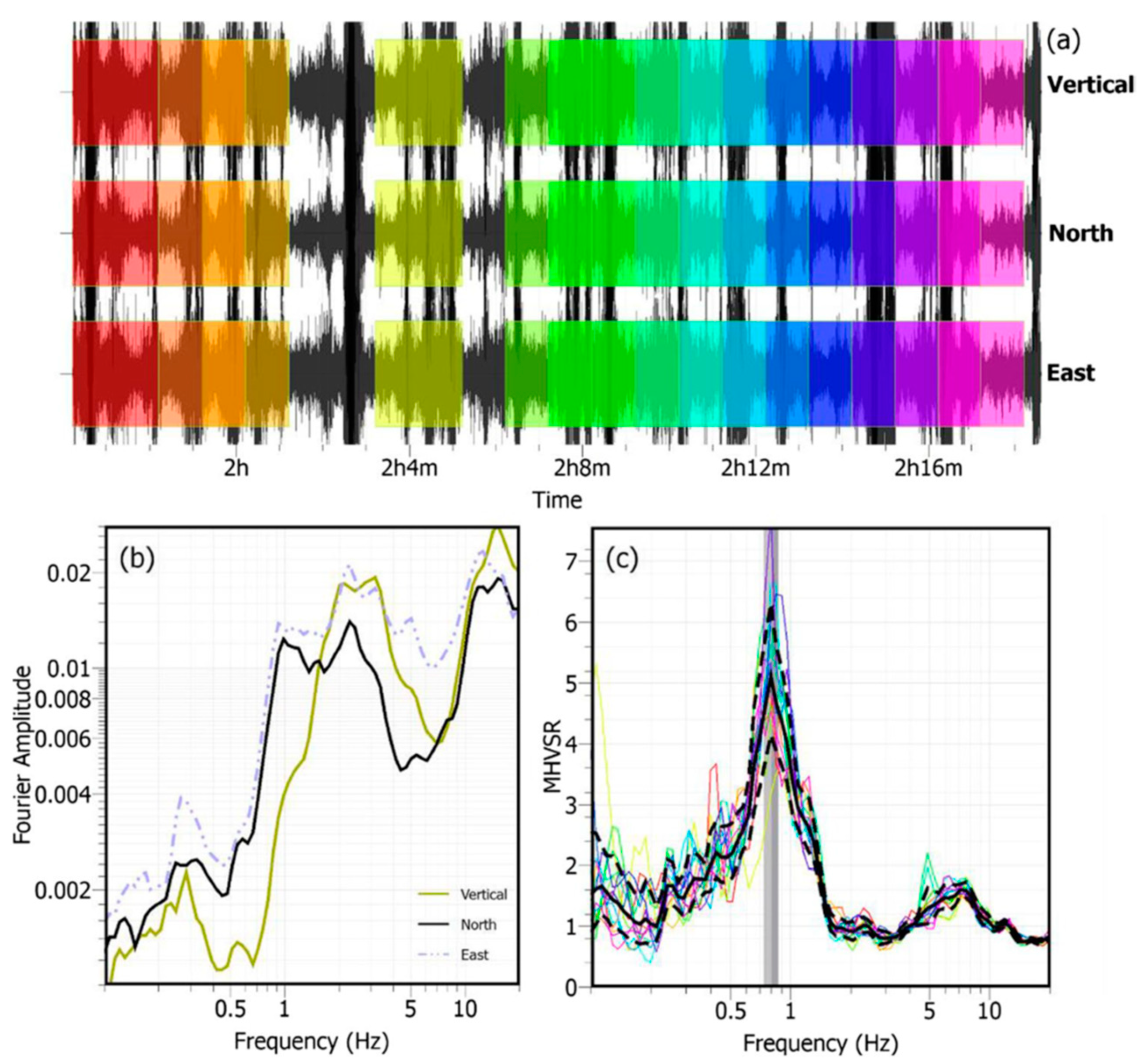
3.2. Horizontal-to-Vertical Spectral Ratio

One of the efficient ways to estimate the fundamental site period is the ratio of the horizontal-to-vertical components (HVSR) of microtremor measurements, namely Nakamura’s method [51]. The method is based on the assumption that the amplification in the horizontal component will be significantly higher than the amplification in the vertical component during seismic wave propagation. Therefore, the peaks of HVSR are associated with site periods. Nakamura updated the theory by including the contributions of surface waves [52] and P waves [53].
Impedance contrasts through the depth of the soil column cause multiple peaks in the HVSR curves. Peaks in the HVSR curve for impedance contrasts greater than four are linked to the horizontal polarization of the fundamental mode Rayleigh wave, coupled with the contribution of the Airy phase of the fundamental mode Love wave [54,55] Thus, sites are grouped in the literature based on the number of peaks in the HVSR curves, (i) without any significant peak, (ii) with one dominant peak, and (iii) with multiple peaks [56]. HVSRs of the considered sites can be calculated by either microtremor measurements (MHVRSs) or recorded earthquake ground motion records (EHVSRs). Kawase et al. [57] compared MHVRS and EHVRS and found similarities up to the first peak frequency. However, there were substantial differences at higher frequencies. The differences were caused by microtremors mainly consisting of surface waves, so the peaks associated with higher modes would not be major.
Empirical studies from different sites have shown that the lowest peak frequency in an MHVSR curve occurs at the fundamental site period [58,59,60]. This requires the use of a spectrum, such as the frequency amplitude spectrum (FAS) [61,62,63], or the 5% damped acceleration response spectrum (PSA) [23,64,65]. Zhu et al. [56] compared the efficiency of both spectra and suggested using the highest peak, not the first one, as the Fourier Amplitude Spectrum (FAS).
The easy-to-use characteristics of the MHVRS method have led to its widespread use in Europe [66,67], New Zealand [68], Turkiye [69,70], North and South America [71,72,73,74], etc. The process for MHVRS analysis is depicted in Figure 1 [75]. The different colors in Figure 1a shows different time windows. In Figure 1c, the mean MHVSR of these time windows were depicted by solid black lines. The dashed black lines represent the mean ± standard deviation.
In addition, several studies have attempted to improve MHVSR to take maximum advantage of the method. Herak [76] suggested using the ratio of S wave to P wave transfer function rather than using S and Rayleigh waves. In their innovative study, Kawase et al. [77] used the diffused field theory to optimize the method. The study demonstrated that the HVSR curve could theoretically be obtained from the imaginary parts of horizontal and vertical Green’s function. It resulted in a similar formula with a scaling factor between horizontal and vertical components at the seismological bedrock. Nagashima et al. [78] effectively used the method to reach an optimal HVSR procedure for subsurface structure investigation. Later, Kawase et al. [79] investigated the validity of theoretical HVSRs for microtremor measurements. It was found that predictions of the diffuse-field theory were generally in line with other methods. Similarly, it was proposed that microtremors form a diffuse field containing all types of body and surface waves [80]. The relative powers of seismic states arise from the equipartition of energy principle. Hence, within a diffuse field, the autocorrelation in the frequency domain is proportional to the imaginary part of Green’s function for source and receiver at the same point. Since average autocorrelations are proportional to average directional energy densities, another method to assess the MHVSR curve was given by Ref. [81], Equation (14), where E1 and E2 are horizontal directional energy densities, and E3 is the vertical one.
M H V S R = E 1 + E 2 E 3
Figure 1. Application of the MHVSR method: (a) windowing, (b) FAS of all components, (c) MHVRS [77].
Geotechnics 03 00071 g001
Since the autocorrelation in the frequency domain is proportional to the imaginary part of Green’s function, MHVSR can be obtained in terms of Green’s function as given by Equation (15), in which ImG parameters represent the imaginary part of Green’s function.
M H V S R = Im G 11 + Im G 22 Im G 33
It was also shown that Green’s function can be used satisfactorily to address lateral discontinuity in return for high computational cost [82,83,84].
Tuan et al. [85] considered several major effects, such as the arrangement of layers and impedance contrast between layers and the half-space, to improve HVSR. Since the suggested formula, Equation (16), was in explicit form, it was stated that it can be considered for direct or inverse problems efficiently. In the equation, I is the impedance value of the layer.
ω p 2 = 1 i = 1 n 1 j = i + 1 n ρ i ρ j V j 2 h i h j + 1 2 i = 1 n h i 2 V i 2 1 2 [ ( i = 1 n ρ i h i ) / I n + 1 i = 1 n 1 j = i + 1 n ρ i ρ j V j 2 h i h j + 1 2 i = 1 n h i 2 V i 2 ]
Equation (16) was simplified as given by Equation (17), where I ( n ) = ρ ¯ V ¯ s * is the average impedance of the layers.
f t = ω p 2 π = V ¯ s 4 h 1 I ( n ) 2 I n + 1 2
Darzi et al. [86] developed an automated method to determine the site’s fundamental resonance to improve HVSR and applied it to the updated Iranian database, as seen in Equation (18).
log 10 ( H V S R ¯ ) j = i = 1 n log 10 ( H V S R ) i j N j
The irregularly spaced microtremor data, which may lead to significant bias in the results due to access and budget restrictions, is another issue for HVSR curves. To address this issue, Cheng et al. [87] proposed employing Voronoi tessellations to obtain an unbiased, statistical representation of T0 from spatially distributed HVSR measurements.
Multiple automated methodologies for the computation of the fundamental site period and its uncertainty using HVSR curves were proposed by Yazdi et al. [14]. The study evaluated current practices, i.e., the use of geometric mean or RotD50, and the use of FAS or PSA. The results showed that being orientation-free is a major advantage for the RotD50 method, and PSA-based HVSR was found to be scenario-dependent. The study proposed four different methods to determine the fundamental site period. The first three methods were individually based on individual HVSR curves, while the last one requires both individual and HVSR curves. The proposed equations for methods 1, 2 and 4 are given below. For the sake of brevity, detailed information about the terms of the following equations and flow chart of the third method is not provided in this review.
  • Method #1
    ln L ( ϕ ) = i = 1 N ln { p ( F P   i j ϕ | ϕ ,   σ ) }
    p ( F P i j | ϕ ,     σ ) = 1 σ 2 π exp [ 1 2 ( ln F P i j ln ϕ σ ) 2 ]
  • Method #2
    ln L ( ϕ ) = i = 1 N w i ln { p ( F P   i j ϕ | ϕ ,   σ ) }
    w i = Prominence   of   P i j φ   from   event   i Sum   of   the   prominences   of   P i j φ   from   all   events
  • Method #3
    ln ( H V S R ) = i = 1 N ln ( H V S R i ) N
As mentioned above, EHVSR is another alternative in the literature for determining the fundamental site period. Several researchers have discussed the similarities between EHVSR and MHVSR in specific regions; however, there are significant differences in other regions. To eliminate these differences, studies have focused on the regression of EHVSR and MHVSR, and the EHVSR-to-MHVSR ratio. Hassani et al. [88] performed regression analyses between the fundamental periods obtained by EHVSR and MHVSR for California, as shown in Equation (24). In the study, it was mentioned that the difference was related to the difference in dominant waves for microtremor and earthquake data.
log 10 ( f d E H V S R ) = ( 0.1 ± 0.03 ) + ( 0.96 ± 0.07 ) log 10 ( f d M H V S R )
Kawase et al. [57] proposed an empirical method, the earthquake-to-microtremor data ratio (EMR), for this purpose. Multiplying the MHVSR by the EMR yields a closer curve to EHVSR. Yong et al. [89] compared Vs30 and T0 values from single-station EMR and multi-station array-based site characterization methods. The results of the study showed that there might be a need to develop site-specific EMR correction factors. The method was employed by Ito et al. [90] for different tectonic settings. Kawase et al. [91] evaluated the effectiveness of the EMR correction for the Grenoble basin.
Even though EHVSR was considered a little bit truer, the amplification of the vertical ground motion component affects it [92,93,94,95].

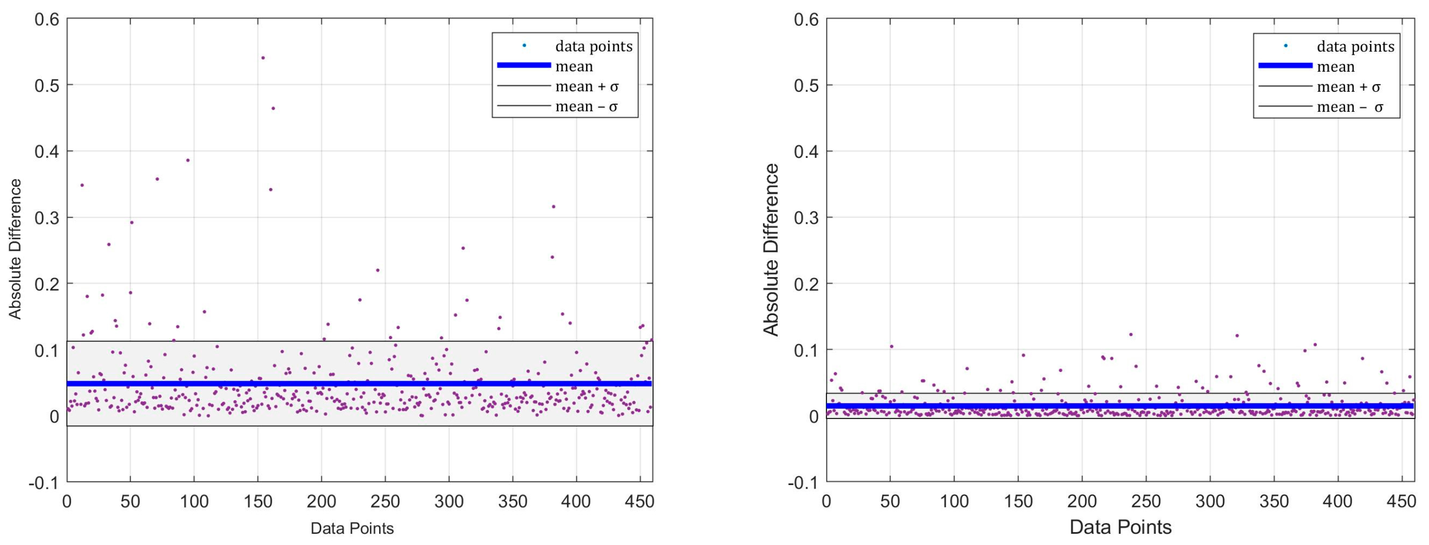
3.3. Data-Driven Method

Databases, such as KiK-net in Japan, provides researchers with invaluable opportunities to apply statistical and theoretical analyses and verify results. Therefore, many data-driven techniques that employ the fundamental site period have been published in the literature, especially for on-site response evaluation [96,97,98,99,100].
Cadet et al. [96] studied the empirical correlations between amplification factors and simple site parameters, T0 and Vsz, where z was 5, 10, 20, and 30 m, obtained from a large subset of the KiK-net. The lowest misfit value was provided by the T0 and Vs30 couple. The data-driven method showed that the best single parameter was also the fundamental site period.
Kaklamanos et al. [101] evaluated critical parameters affecting bias in site-response analyses based on KiK-net downhole array data, where the fundamental site frequency/period was also considered a critical parameter. The study concluded that the most influential parameters were maximum shear strain in the soil profile, observed peak ground acceleration at the ground surface, and the predominant spectral period of the ground surface.
Mousavi Anzehaee et al. [102] used the Bayesian data fusion method and a database to estimate the fundamental site period. The results of different data windows were employed for fusion. It was stated that the method does not require additional filters but rather a simple band-pass filter. The results showed that the method is a high-performance and easy-to-apply technique.
Zhu et al. [103] released an open-source database of strong-motion stations in Japan, in which the EHVSRs of each station were given in detail. Zhu et al. [104] evaluated the goodness of earthquake site response predictions using1725 K-NET and KiK-net sites in Japan. Therefore, the random forest algorithm was employed to perform multivariate non-parametric and nonlinear regressions in addition to conventional regression analyses. In the study, the peak period of the EHVSR was considered the fundamental site period. It was mentioned that two types of uncertainty: (i) modeling uncertainty arising from simplifications, assumptions, and approximations, and (ii) parametric uncertainty related to the input parameters and model coefficients, influence the predictions. Later, Zhu et al. [105] compared the success of machine learning and physics-based modeling techniques. The results showed that the supervised learning technique, which requires a few input parameters, is superior to detailed 1D ground response analyses.
In practice, the basic 4H/V equation is preferred owing to its simplicity. However, as mentioned above, this equation overestimates the fundamental site period by 20%. Therefore, Güllü and Hasanoğlu [106] proposed a best-fit coefficient for the total travel time, which resulted in a minimum standard deviation for 459 KiK-net stations. The study proposed a simple yet more accurate equation based on statistical analyses, as shown in Equation (25). The residuals of the original and improved equations were compared in Figure 2 to exemplify the improvement.
T 0 = 3.51 H V
Although it was shown in the literature that the use of Vs30 is not self-sufficient for soil classification. However, many studies have been performed to determine Vs30 in the literature since the seismic codes dictate the use of this term. Therefore, Güllü et al. [107] developed a data-driven methodology to take advantage of the previously performed studies on Vs30, which is not suitable by itself, to calculate the fundamental site period. In this study, the soil column is first divided into two segments at a depth of 30 m, Figure 3a. The upper part of the soil column is linked to the Vs30, while the bottom part is associated with engineering bedrock depth. Two different depths, namely 760 (Z0.76) and 1000 m (Z1.0), were considered as bedrock in the study. In the second step, the soil column was reduced to a two-degree-of-freedom system, Figure 3b. Finally, the two-degree-of-freedom system condensed to a single-degree-of-freedom system again, Figure 3c.
Based on the solution of the undamped equation of motion for the resulting single-degree-of-freedom system, the fundamental site periods were obtained as given by Equations (26) and (27). The method is highly suitable for large-scale applications with physics-informed machine-learning techniques.
T 0.76 = 2 π 0.76 M e f f 0.76 K e f f = 2 π 0.3268 × Z 0.76 ( 1 0.07965 × V s 30 2 18.66 × V s 30 + 2514 + Z 0.76 30 6.974 × 10 5 ) 1
T 1.0 = 2 π 1.0 M e f f 1.0 K e f f = 2 π 0.3342 × Z 1.0 ( 1 0.07448 × V s 30 2 14.94 × V s 30 + 1991 + Z 1.0 30 7.101 × 10 5 ) 1

4. Discussion

In this review, various approaches for determining the site fundamental period, including analytical methods, Horizontal-to-Vertical Spectral Ratio (HVSR), and data-driven techniques, were critically examined. Analytical methods offer nearly exact solutions, but their computational demands can become prohibitively expensive, especially when applied over wide-ranging scenarios rather than individual points.
Even though the site fundamental period was mainly preferred for the development of ground motion prediction equations as a single parameter or proxy, novel structural design methods showed that the fundamental site period is significantly important in determining the resonance risk, which imparts maximum seismic energy to a structure [108,109,110]. Expressly, seismic energy imparted to a structure is related to fundamental periods/frequencies of the structure, soil, and ground motion, as shown in Figure 4.
The HVSR method has gained widespread acceptance due to its simplicity, cost-effectiveness, sensitivity to in-situ conditions, and suitability for microzonation studies. However, it does have drawbacks, including sensitivity to noise and depth, with a particular sensitivity to shallow subsurface conditions. Furthermore, its accuracy tends to decrease at higher frequencies, limiting its applicability under certain conditions.
Data-driven methods, such as the approach outlined in Reference [107], present practical tools, particularly for regional studies. Nevertheless, these methods introduce a level of uncertainty into the analysis that should be quantified to take advantage of these methods.
Finally, the selection of an appropriate method to determine the site’s fundamental period should be guided by the specific requirements and constraints of the seismic analysis being undertaken.

5. Conclusions

This study combined the studies aimed at determining the site’s fundamental period and understanding its importance. A wide range of studies, from those proposing the simplest equations to the most complex ones, are summarized in this review. All these studies agree on the importance of the fundamental site period for several purposes. However, there are still some discussions on the procedures. In the literature, the site’s fundamental period was determined mainly by frequency amplitude and pseudo-acceleration spectra when employing the HVSR method. However, using the seismic input energy spectrum to determine the fundamental site period would reduce uncertainties.
In general, the fundamental site period is determined by one-dimensional analyses. In many cases, this may not be sufficient due to local geological irregularities/discontinuities. Finally, all existing data should be examined to find alternative procedures for determining fundamental site periods at the community/city level where three-dimensional surface and subsurface topography are rapidly varying.

Funding

This research received no external funding.

Data Availability Statement

No new data were created or analyzed in this study. Data sharing is not applicable to this article.

Conflicts of Interest

The author declares no conflict of interest.

References

  1. Kitazawa, G. Damages to the wooden houses in the City of Tokyo and its suburbs. Bull. Earthq. Investig. Commun. 1926, 100, 1–126. (In Japanese) [Google Scholar]
  2. Kramer, S.L. Geotechnical Earthquake Engineering; Prentice Hall: Upper Saddle River, NJ, USA, 1996. [Google Scholar]
  3. Deniz, A.; Yüksel, E.; Çelik, O.C.; Çakır, Z.; Yaltırak, C.; Serter, E.; Yıldırım, H.; Güllü, A. 30.10.2020 Izmir Earthquake Evaluation Report; Istanbul Technical University: Istanbul, Turkey, 2020. (In Turkish) [Google Scholar]
  4. Beresnev, I.A.; Wen, K.L. Nonlinear soil response-A reality? Bull. Seismol. Soc. Am. 1996, 86, 1964–1978. [Google Scholar] [CrossRef]
  5. Borcherdt, R.D. Effects of local geology on ground motion near San Francisco Bay. Bull. Seismol. Soc. Am. 1970, 60, 29–61. [Google Scholar]
  6. Kagami, H.; Duke, C.M.; Liang, G.C.; Ohta, Y. Evaluation of site effect upon seismic wave amplification due to extremely deep soil deposits. Bull. Seismol. Soc. Am. 1982, 72, 987–998. [Google Scholar] [CrossRef]
  7. Bard, P.Y.; Bouchon, M. The seismic response of sediment-filled valleys. Part I. The case of incident SH waves. Bull. Seismol. Soc. Am. 1980, 70, 1263–1286. [Google Scholar] [CrossRef]
  8. Housner, G.W. Behavior of structures during earthquakes. J. Eng. Mech. Div. ASCE 1959, EM4, 109–129. [Google Scholar] [CrossRef]
  9. Goda, K.; Kiyota, T.; Pokhrel, R.M.; Chiaro, G.; Katagiri, T.; Sharma, K.; Wilkinson, S. The 2015 Gorkha Nepal earthquake: Insights from earthquake damage survey. Front. Built Environ. 2015, 1, 8. [Google Scholar] [CrossRef]
  10. Beck, J.L.; HallJ, F. Factors contributing to the catastrophe in Mexico City during the earthquake of September 19, 1985. Geophys. Res. Lett. 1986, 3, 593–596. [Google Scholar] [CrossRef]
  11. Kawase, H. Irregular ground analysis to interpret time-characteristics of strong motion recorded in Mexico City during 1985 Mexico earthquake. Dev. Geotech. Eng. 1987, 44, 467–476. [Google Scholar]
  12. Panzera, F.; Lombardo, G.; Imposa, S.; Grassi, S.; Gresta, S.; Catalano, S.; Romagnoli, G.; Tortorici, G.; Patti, F.; Di Maio, E. Correlation between earthquake damage and seismic site effect: The study case of Lentini and Carlentini, Italy. Eng. Geol. 2018, 240, 149–162. [Google Scholar] [CrossRef]
  13. AFAD Disaster and Emergency Management Authority of Turkey. Available online: https://deprem.afad.gov.tr/tarihteBuAy?id=25 (accessed on 27 September 2023). (In Turkish)
  14. Yazdi, M.; Motamed, R.; Anderson, J.G. A New Set of Automated Methodologies for Estimating Site Fundamental Frequency and Its Uncertainty Using Horizontal-to-Vertical Spectral Ratio Curves. Seismol. Res. Lett. 2022, 93, 1721–1736. [Google Scholar] [CrossRef]
  15. Zhu, C.; Pilz, M.; Cotton, F. Which is a better proxy, site period or depth to bedrock, in modeling linear site response in addition to the average shear-wave velocity? Bull. Earthq. Eng. 2020, 18, 797–820. [Google Scholar] [CrossRef]
  16. Hassani, B.; Atkinson, G.M. Applicability of the NGAwest2 site-effects model for central and eastern North America. Bull. Seismol. Soc. Am. 2016, 106, 1331–1341. [Google Scholar] [CrossRef]
  17. Hassani, B.; Atkinson, G.M. Applicability of the site fundamental frequency as a VS30 proxy for central and eastern North America. Bull. Seismol. Soc. Am. 2016, 106, 653–664. [Google Scholar] [CrossRef]
  18. Hassani, B.; Atkinson, G.M. Site-effects model for central and eastern North America based on peak frequency. Bull. Seismol. Soc. Am. 2016, 106, 2197–2213. [Google Scholar] [CrossRef]
  19. Zhao, J.X.; Xu, H. A comparison of VS30 and site period as site effect parameters in response spectral ground-motion prediction equations. Bull. Seismol. Soc. Am. 2013, 103, 1. [Google Scholar] [CrossRef]
  20. Pitilakis, K.; Riga, E.; Anastasiadis, A. New code site classification, amplification factors and normalized response spectra based on a worldwide ground-motion database. Bull. Earthq. Eng. 2013, 11, 925–966. [Google Scholar] [CrossRef]
  21. Hassani, B.; Atkinson, G.M. Application of a site-effects model based on peak frequency and average shear-wave velocity to California. Bull. Seismol. Soc. Am. 2018, 108, 351–357. [Google Scholar] [CrossRef]
  22. Luzi, L.; Puglia, R.; Pacor, F.; Gallipoli, M.; Bindi, D.; Mucciarelli, M. Proposal for a soil classification based on parameters alternative or complementary to Vs30. Bull. Earthq. Eng. 2011, 9, 1877–1898. [Google Scholar] [CrossRef]
  23. Wang, Y.S.; Shi, Y.; Jiang, W.P.; Yao, E.L.; Miao, Y. Estimating site fundamental period from shear-wave velocity profile. Bull. Seismol. Soc. Am. 2018, 108, 3431–3445. [Google Scholar] [CrossRef]
  24. Borja, R.I.; Chao, H.-Y.; Montáns, F.J.; Lin, C.-H. Nonlinear ground response at Lotung LSST site. J. Geotech. Geoenviron. Eng. 1999, 125, 187–197. [Google Scholar] [CrossRef]
  25. Baturay, M.B.; Stewart, J.P. Uncertainty and bias in ground-motion estimates from ground response analyses. Bull. Seismol. Soc. Am. 2003, 93, 2025–2042. [Google Scholar] [CrossRef]
  26. Lee, C.-P.; Tsai, Y.-B.; Wen, K.-L. Analysis of nonlinear site response using the LSST downhole accelerometer array data. Soil Dyn. Earthq. Eng. 2006, 26, 435–460. [Google Scholar] [CrossRef]
  27. Tsai, C.-C.; Hashash, Y.M. Learning of dynamic soil behavior from downhole arrays. J. Geotech. Geoenviron. Eng. 2009, 135, 745–757. [Google Scholar] [CrossRef]
  28. Thompson, E.M.; Baise, L.G.; Tanaka, Y.; Kayen, R.E. A taxonomy of site response complexity. Soil Dyn. Earthq. Eng. 2012, 41, 32–43. [Google Scholar] [CrossRef]
  29. Yee, E.; Stewart, J.P.; Tokimatsu, K. Elastic and large-strain nonlinear seismic site response from analysis of vertical array recordings. J. Geotech. Geoenviron. Eng. 2013, 139, 1789–1801. [Google Scholar] [CrossRef]
  30. Kaklamanos, J.; Baise, L.G.; Thompson, E.M.; Dorfmann, L. Comparison of 1-D linear, equivalent-linear, and nonlinear site response models at six KiK-net validation sites. Soil Dyn. Earthq. Eng. 2015, 69, 207–219. [Google Scholar] [CrossRef]
  31. Pinzón, L.A.; Leiva, D.A.H.; Moya-Fernández, A.; Schmidt-Díaz, V.; Pujades, L.G. Seismic site classification of the Costa Rican Strong-Motion Network based on V S30 measurements and site fundamental period. Earth Sci. Res. J. 2021, 25, 383–389. [Google Scholar] [CrossRef]
  32. Benjumea, B.; Hunter, J.A.; Pullan, S.E.; Brooks, G.R.; Pyne, M.; Aylsworth, J.M. VS30 and fundamental site period estimates in soft sediments of the Ottawa Valley from near-surface geophysical measurements. J. Environ. Eng. Geophys. 2008, 13, 313–323. [Google Scholar] [CrossRef]
  33. Laouami, N. Vertical ground motion prediction equations and vertical-to-horizontal (V/H) ratios of PGA and PSA for Algeria and surrounding region. Bull. Earthq. Eng. 2019, 17, 3637–3660. [Google Scholar] [CrossRef]
  34. Chousianitis, K.; Del Gaudio, V.; Pierri, P.; Tselentis, G.A. Regional ground-motion prediction equations for amplitude-, frequency response-, and duration-based parameters for Greece. Earthq. Eng. Struct. Dyn. 2018, 47, 2252–2274. [Google Scholar] [CrossRef]
  35. Alessandro, C.D.; Bonilla, L.F.; Boore, D.M.; Rovelli, A.; Scotti, O. Predominant-Period Site Classification for Response Spectra Prediction Equations in Italy. Bull. Seismol. Soc. Am. 2012, 102, 680–695. [Google Scholar] [CrossRef]
  36. Seyhan, E.; Stewart, J.P. Semi-empirical nonlinear site amplification from NGA-West2 data and simulations. Earthq. Spectra 2014, 30, 1241–1256. [Google Scholar] [CrossRef]
  37. Hassani, B.; Atkinson, G.M. Site-effects model for central and eastern North America based on peak frequency and average shear-wave velocity. Bull. Seismol. Soc. Am. 2018, 108, 338–350. [Google Scholar] [CrossRef]
  38. Yazdi, M.; Anderson, J.G.; Motamed, R. Reducing the uncertainties in the NGA-West2 ground motion models by incorporating the frequency and amplitude of the fundamental peak of the horizontal-to-vertical spectral ratio of surface ground motions. Earthq. Spectra 2023, 39, 1088–1108. [Google Scholar] [CrossRef]
  39. Kotha, S.R.; Cotton, F.; Bindi, D. A new approach to site classification: Mixed-effects Ground Motion Prediction Equation with spectral clustering of site amplification functions. Soil Dyn. Earthq. Eng. 2018, 110, 318–329. [Google Scholar] [CrossRef]
  40. Kwak, D.Y.; Seyhan, E. Two-stage nonlinear site amplification modeling for Japan with VS 30 and fundamental frequency dependency. Earthq. Spectra 2020, 36, 1359–1385. [Google Scholar] [CrossRef]
  41. Ambraseys, N.N. A note on the response of an elastic overburden of varying rigidity to an arbitrary ground motion. Bull. Seismol. Soc. Am. 1959, 49, 211–220. [Google Scholar] [CrossRef]
  42. Idriss, I.M.; Seed, H.B. Seismic response of horizontal soil layers. J. Soil Mech. Found. Div. 1968, 94, 1003–1034. [Google Scholar] [CrossRef]
  43. Madera, G.A. Fundamental Period and Peak Accelerations in Layered Systems; Research Report R70–37; Department of Civil Engineering, MIT: Cambridge, MA, USA, 1971. [Google Scholar]
  44. Hadjian, A.H. Fundamental period and mode shape of layered soil profiles. Soil Dyn. Earthq. Eng. 2002, 22, 885–891. [Google Scholar] [CrossRef]
  45. Dobry, R.; Oweis, I.; Urzua, A. Simplified procedures for estimating the fundamental period of a soil profile. Bull. Seismol. Soc. Am. 1976, 66, 1293–1321. [Google Scholar]
  46. Motazedian, D.K.; Hunter, B.J.; Sivathayalam, S.; Crow, H.; Brooks, G. Comparison of site periods derived from different evaluation methods. Bull. Seismol. Soc. Am. 2011, 101, 2492–2954. [Google Scholar] [CrossRef]
  47. Urzua, A.; Dobry, R.; Christian, J. Is harmonic averaging of shear wave velocity or the simplified Rayleigh method appropriate to estimate the period of a soil profile. Earthq. Spectra 2017, 33, 895–915. [Google Scholar] [CrossRef]
  48. Gazetas, G. Vibrational characteristics of soil deposits with variable wave velocity. Int. J. Numer. Anal. Methods Geomech. 1982, 6, 1–20. [Google Scholar] [CrossRef]
  49. Biggs, J.M. Introduction to Structural Dynamics; McGraw Hill: New York, NY, USA, 1964. [Google Scholar]
  50. Building Center of Japan (BCJ). Building Standard Law; Building Center of Japan (BCJ): Tokyo, Japan, 2005. [Google Scholar]
  51. Nakamura, Y. A method for dynamic characteristics estimation of subsurface using microtremor on the ground surface. Q. Rep. Railw. Tech. Res. Inst. 1989, 30, 25–33. [Google Scholar]
  52. Nakamura, Y. Real-time information systems for seismic hazards mitigation UrEDAS, HERAS and PIC. Q. Rep.-Rtri 1996, 37, 112–127. [Google Scholar]
  53. Nakamura, Y. Clear identification of fundamental idea of Nakamura’s technique and its applications. In Proceedings of the 12th World Conference on Earthquake Engineering, Auckland, New Zealand, 30 January–4 February 2000; pp. 1–8. [Google Scholar]
  54. Lunedei, E.; Albarello, D. Theoretical HVSR curves from full wavefield modelling of ambient vibrations in a weakly dissipative layered Earth. Geophys. J. Int. 2010, 181, 1093–1108. [Google Scholar] [CrossRef]
  55. Konno, K.; Ohmachi, T. Ground-motion characteristics estimated from spectral ratio between horizontal and vertical components of microtremor. Bull. Seismol. Soc. Am. 1998, 88, 228–241. [Google Scholar] [CrossRef]
  56. Zhu, C.; Cotton, F.; Pilz, M. Detecting site resonant frequency using HVSR: Fourier versus response spectrum and the first versus the highest peak frequency. Bull. Seismol. Soc. Am. 2020, 110, 427–440. [Google Scholar] [CrossRef]
  57. Kawase, H.; Mori, Y.; Nagashima, F. Difference of horizontal-to-vertical spectral ratios of observed earthquakes and microtremors and its application to S-wave velocity inversion based on the diffuse field concept. Earth Planets Space 2018, 70, 1. [Google Scholar] [CrossRef]
  58. Field, E.; Jacob, K. The theoretical response of sedimentary layers to ambient seismic noise. Geophys. Res. Lett. 1993, 20, 2925–2928. [Google Scholar] [CrossRef]
  59. Bour, M.; Fouissac, D.; Dominique, P.; Martin, C. On the use of microtremor recordings in seismic microzonation. Soil Dyn. Earthq. Eng. 1998, 17, 465–474. [Google Scholar] [CrossRef]
  60. Haghshenas, E.; Bard, P.Y.; Theodulidis, N. Sesame WP04 Team. Empirical evaluation of microtremor H/V spectral ratio. Bull. Earthq. Eng. 2008, 6, 75–108. [Google Scholar] [CrossRef]
  61. Molnar, S.; Cassidy, J.F. A comparison of site response techniques using weak-motion earthquakes and microtremors. Earthq. Spectra 2006, 22, 169–188. [Google Scholar] [CrossRef]
  62. Bard, P.-Y.; Acerra, C.; Aguacil, G.; Anastasiadis, A.; Atakan, K.; Azzara, R.; Basili, E.; Bertrand, B.; Bettig, B.; Blarel, F.; et al. Guidelines for the implementation of the H/V spectral ratio technique on ambient vibrations measurements, processing and interpretation. Bull. Earthq. Eng. 2008, 6, 1–2. [Google Scholar] [CrossRef]
  63. Kwak, Y.; Stewart, J.P.; Mandokhail, S.J.; Park, D. Supplementing VS30 with H/V spectral ratios for predicting site effects. Bull. Seismol. Soc. Am. 2017, 107, 2028–2042. [Google Scholar] [CrossRef]
  64. Ghofrani, H.; Atkinson, G.M.; Goda, K. Implications of the 2011 M9. 0 Tohoku Japan earthquake for the treatment of site effects in large earthquakes. Bull. Earthq. Eng. 2013, 11, 171–203. [Google Scholar] [CrossRef]
  65. Ghofrani, H.; Atkinson, G.M. Site condition evaluation using horizontal-to-vertical response spectral ratios of earthquakes in the NGA-West 2 and Japanese databases. Soil Dyn. Earthq. Eng. 2014, 67, 30–43. [Google Scholar] [CrossRef]
  66. Acerra, C.; Aguacil, G.; Anastasiadis, A.; Atakan, K.; Azzara, R.; Bard, P.Y.; Zacharopoulos, S. Guidelines for the Implementation of the H/V Spectral Ratio Technique on Ambient Vibrations Measurements, Processing and Interpretation; EVG1-CT-2000-00026 SESAME; European Commission: Brussels, Belgium, 2004; Available online: http://sesame.geopsy.org/Delivrables/Del-D23-HV_User_Guidelines.pdf (accessed on 27 September 2023).
  67. Bard, P.Y. The H/V technique: Capabilities and limitations based on the results of the SESAME project. Bull. Earthq. Eng. 2008, 6, 1–2. [Google Scholar] [CrossRef]
  68. Vantassel, J.; Cox, B.; Wotherspoon, L.; Stolte, A. Mapping depth to bedrock, shear stiffness, and fundamental site period at CentrePort, Wellington, using surface-wave methods: Implications for local seismic site amplification. Bull. Seismol. Soc. Am. 2018, 108, 1709–1721. [Google Scholar] [CrossRef]
  69. Özalaybey, S.; Zor, E.; Ergintav, S.; Tapırdamaz, M.C. Investigation of 3-D basin structures in the Izmit Bay area (Turkey) by single-station microtremor and gravimetric methods. Geophys. J. Int. 2011, 186, 883–894. [Google Scholar] [CrossRef]
  70. Eskişar, T.; Özyalin, Ş.; Kuruoǧlu, M.; Yilmaz, H.R. Microtremor measurements in the northern coast of Izmir Bay, Turkey to evaluate site-specific characteristics and fundamental periods by H/V spectral ratio method. J. Earth Syst. Sci. 2013, 122, 123–136. [Google Scholar] [CrossRef]
  71. Pilz, M.; Parolai, S.; Leyton, F.; Campos, J.; Zschau, J. A comparison of site response techniques using earthquake data and ambient seismic noise analysis in the large urban areas of Santiago de Chile. Geophys. J. Int. 2009, 178, 713–728. [Google Scholar] [CrossRef]
  72. Leyton, F.; Ruiz, S.; Sepúlveda, S.A.; Contreras, J.P.; Rebolledo, S.; Astroza, M. Microtremors’ HVSR and its correlation with surface geology and damage observed after the 2010 Maule earthquake (Mw 8.8) at Talca and Curicó, Central Chile. Eng. Geol. 2013, 161, 26–33. [Google Scholar] [CrossRef]
  73. Stephenson, W.J.; Asten, M.W.; Odum, J.K.; Frankel, A.D. Shear-wave velocity in the Seattle Basin to 2 km depth characterized with the krSPAC microtremor array method: Insights for urban basin-scale imaging. Seismol. Res. Lett. 2019, 90, 1230–1242. [Google Scholar] [CrossRef]
  74. Teague, D.P.; Cox, B.R.; Rathje, E.M. Measured vs. predicted site response at the Garner Valley Downhole Array considering shear wave velocity uncertainty from borehole and surface wave methods. Soil Dyn. Earthq. Eng. 2018, 113, 339–355. [Google Scholar] [CrossRef]
  75. Molnar, S.; Sirohey, A.; Assaf, J.; Bard, P.Y.; Castellaro, S.; Cornou, C.; Cox, B.; Guillier, B.; Hassani, B.; Kawase, H. A review of the microtremor horizontal-to-vertical spectral ratio (MHVSR) method. J. Seismol. 2022, 26, 653–685. [Google Scholar] [CrossRef]
  76. Herak, M. ModelHVSR—A Matlab® tool to model horizontal-to-vertical spectral ratio of ambient noise. Comput. Geosci. 2008, 34, 1514–1526. [Google Scholar] [CrossRef]
  77. Kawase, H.; Sánchez-Sesma, F.J.; Matsushima, S. The optimal use of horizontal-to-vertical spectral ratios of earthquake motions for velocity inversions based on diffuse-field theory for plane waves. Bull. Seismol. Soc. Am. 2011, 101, 2001–2014. [Google Scholar] [CrossRef]
  78. Nagashima, F.; Matsushima, S.; Kawase, H.; Sánchez-Sesma, F.J.; Hayakawa, T.; Satoh, T.; Oshima, M. Application of horizontal-to-vertical spectral ratios of earthquake ground motions to identify subsurface structures at and around the K-NET site in Tohoku, Japan. Bull. Seismol. Soc. Am. 2014, 104, 2288–2302. [Google Scholar] [CrossRef]
  79. Kawase, H.; Matsushima, S.; Satoh, T.; Sánchez-Sesma, F.J. Applicability of theoretical horizontal-to-vertical ratio of microtremors based on the diffuse field concept to previously observed data. Bull. Seismol. Soc. Am. 2015, 105, 3092–3103. [Google Scholar] [CrossRef]
  80. Sánchez-Sesma, F.J.; Rodríguez, M.; Iturrarán-Viveros, U.; Luzón, F.; Campillo, M.; Margerin, L.; García-Jerez, A.; Suarez, M.; Santoyo, M.A.; Rodríguez-Castellanos, A. A theory for microtremor H/V spectral ratio: Application for a layered medium. Geophys. J. Int. 2011, 186, 221–225. [Google Scholar] [CrossRef]
  81. Arai, H.; Tokimatsu, K. S-wave velocity profiling by inversion of microtremor H/V spectrum. Bull. Seismol. Soc. Am. 2004, 94, 53–63. [Google Scholar] [CrossRef]
  82. Spica, Z.; Caudron, C.; Perton, M.; Lecocq, T.; Camelbeeck, T.; Legrand, D.; Piña-Flores, J.; Iglesias, A.; Syahbana, D.K. Velocity models and site effects at Kawah Ijen volcano and Ijen caldera (Indonesia) determined from ambient noise cross-correlations and directional energy density spectral ratios. J. Volcanol. Geotherm. Res. 2015, 302, 173–189. [Google Scholar] [CrossRef]
  83. Spica, Z.J.; Perton, M.; Nakata, N.; Liu, X.; Beroza, G.C. Site characterization at Groningen gas field area through joint surface-borehole H/V analysis. Geophys. J. Int. 2018, 212, 412–421. [Google Scholar] [CrossRef]
  84. Spica, Z.; Perton, M.; Nakata, N.; Liu, X.; Beroza, G.C. Shallow VS imaging of the Groningen area from joint inversion of multimode surface waves and H/V spectral ratios. Seismol. Res. Lett. 2018, 89, 1720–1729. [Google Scholar] [CrossRef]
  85. Tuan, T.T.; Vinh, P.C.; Ohrnberger, M.; Malischewsky, P.; Aoudia, A. An improved formula of fundamental resonance frequency of a layered half-space model used in H/V ratio technique. Pure Appl. Geophys. 2016, 173, 2803–2812. [Google Scholar] [CrossRef]
  86. Darzi, A.; Pilz, M.; Zolfaghari, M.R.; Fäh, D. An automatic procedure to determine the fundamental site resonance: Application to the Iranian strong motion network. Pure Appl. Geophys. 2019, 176, 3509–3531. [Google Scholar] [CrossRef]
  87. Cheng, T.; Hallal, M.M.; Vantassel, J.P.; Cox, B.R. Estimating unbiased statistics for fundamental site frequency using spatially distributed HVSR measurements and Voronoi tessellation. J. Geotech. Geoenviron. Eng. 2021, 147, 04021068. [Google Scholar] [CrossRef]
  88. Hassani, B.; Yong, A.; Atkinson, G.M.; Feng, T.; Meng, L. Comparison of site dominant frequency from earthquake and microseismic data in California. Bull. Seismol. Soc. Am. 2019, 109, 1034–1040. [Google Scholar] [CrossRef]
  89. Yong, A.; Ngashima, F.; Ito, E.; Kawase, H.; Fletcher, J.B.; Hayashi, K.; Martin, A.J.; Grant, A. Comparison of VS30 and f0 values from single station earthquake-to-microtremor ratio (EMR) and multi-station array-based site characterization methods. In Proceedings of the AGU Fall Meeting Abstracts, Online, 7–11 December 2020; p. S002-0006. [Google Scholar]
  90. Ito, E.; Cornou, C.; Nagashima, F.; Kawase, H. Estimation of velocity structures in the Grenoble Basin, France, using pseudo earthquake horizontal-to-vertical spectral ratio from microtremors. Bull. Seismol. Soc. Am. 2021, 111, 627–653. [Google Scholar] [CrossRef]
  91. Kawase, H.; Nagashima, F.; Ito, E.; Cornou, C. S-Wave Velocity Inversion Based on Microtremor HVR: Effectiveness of the EMR Correction for the Grenoble Basin. In Earthquake Geotechnical Engineering for Protection and Development of Environment and Constructions; CRC Press: Boca Raton, FL, USA, 2019; pp. 3250–3258. [Google Scholar]
  92. Lermo, J.; Chávez-García, F.J. Site effect evaluation using spectral ratios with only one station. Bull. Seismol. Soc. Am. 1993, 83, 1574–1594. [Google Scholar] [CrossRef]
  93. Parolai, S.; Bindi, D.; Augliera, P. Application of the generalized inversion technique (GIT) to a microzonation study: Numerical simulations and comparison with different site-estimation techniques. Bull. Seismol. Soc. Am. 2000, 90, 286–297. [Google Scholar] [CrossRef]
  94. Raptakis, D.; Chávez-Garcıa, F.J.; Makra, K.; Pitilakis, K. Site effects at Euroseistest—I. Determination of the valley structure and confrontation of observations with 1D analysis. Soil Dyn. Earthq. Eng. 2000, 19, 1–22. [Google Scholar] [CrossRef]
  95. Rong, M.; Li, H.; Yu, Y. The difference between horizontal-to-vertical spectra ratio and empirical transfer function as revealed by vertical arrays. PLoS ONE 2019, 14, e0210852. [Google Scholar] [CrossRef]
  96. Cadet, H.; Bard, P.-Y.; Duval, A.M.; Bertrand, E. Site effect assessment using KiK-net data: Part 2—Site amplification prediction equation based on f0 and Vsz. Bull. Earthq. Eng. 2012, 10, 451–489. [Google Scholar] [CrossRef]
  97. Kokusho, T.; Sato, K. Surface-to-base amplification evaluated from KiK-net vertical array strong motion records. Soil Dyn. Earthq. Eng. 2008, 28, 707–716. [Google Scholar] [CrossRef]
  98. Régnier, J.; Bonilla, L.F.; Bertrand, E.; Semblat, J.F. Influence of the VS profiles beyond 30 m depth on linear site effects: Assessment from the KiK-net data. Bull. Seismol. Soc. Am. 2014, 104, 2337–2348. [Google Scholar] [CrossRef]
  99. Régnier, J.; Cadet, H.; Bonilla, L.F.; Bertrand, E.; Semblat, J.F. Assessing nonlinear behavior of soils in seismic site response: Statistical analysis on KiK-net strong-motion data. Bull. Seismol. Soc. Am. 2013, 103, 1750–1770. [Google Scholar] [CrossRef]
  100. Han, B.; Yang, Z.; Zdravkovic, L.; Kontoe, S. Non-linearity of gravelly soils under seismic compressional deformation based on KiK-net downhole array observations. Geotech. Lett. 2015, 5, 287–293. [Google Scholar] [CrossRef]
  101. Kaklamanos, J.; Bradley, B.A.; Thompson, E.M.; Baise, L.G. Critical parameters affecting bias and variability in site-response analyses using KiK-net downhole array data. Bull. Seismol. Soc. Am. 2013, 103, 1733–1749. [Google Scholar] [CrossRef]
  102. Mousavi Anzehaee, M.; Heydarzadeh, K.; Adib, A. Employing the Bayesian data fusion to estimate the fundamental frequency of site by means of microtremor data. Acta Geod. Geophys. 2018, 53, 523–541. [Google Scholar] [CrossRef]
  103. Zhu, C.; Weatherill, G.; Cotton, F.; Pilz, M.; Kwak, D.Y.; Kawase, H. An open-source site database of strong-motion stations in Japan: K-NET and KiK-net (v1. 0.0). Earthq. Spectra 2021, 37, 2126–2149. [Google Scholar] [CrossRef]
  104. Zhu, C.; Cotton, F.; Kawase, H.; Haendel, A.; Pilz, M.; Nakano, K. How well can we predict earthquake site response so far? Site-specific approaches. Earthq. Spectra 2022, 38, 1047–1075. [Google Scholar] [CrossRef]
  105. Zhu, C.; Cotton, F.; Kawase, H.; Nakano, K. How well can we predict earthquake site response so far? Machine learning vs physics-based modeling. Earthq. Spectra 2023, 39, 478–504. [Google Scholar] [CrossRef]
  106. Güllü, A.; Hasanoğlu, S. A statistical investigation to determine dominant frequency of layered soil profiles. Turk. J. Eng. 2022, 6, 95–105. [Google Scholar] [CrossRef]
  107. Güllü, A.; Hasanoğlu, S.; Yüksel, E. A Practical Methodology to Estimate Site Fundamental Periods Based on the KiK-net Borehole Velocity Profiles and Its Application to Istanbul. Bull. Seismol. Soc. Am. 2022, 112, 2606–2620. [Google Scholar] [CrossRef]
  108. Güllü, A.; Yüksel, E.; Yalçın, C.; Anıl Dindar, A.; Özkaynak, H.; Büyüköztürk, O. An improved input energy spectrum verified by the shake table tests. Earthq. Eng. Struct. Dyn. 2019, 48, 27–45. [Google Scholar] [CrossRef]
  109. Güllü, A.; Yüksel, E.; Yalcin, C.; Buyukozturk, O. Damping effect on seismic input energy and its verification by shake table tests. Adv. Struct. Eng. 2021, 24, 2669–2683. [Google Scholar] [CrossRef]
  110. Hasanoğlu, S.; Güllü, E.; Güllü, A. Empirical correlations of constant ductility seismic input and hysteretic energies with conventional intensity measures. Bull. Earthq. Eng. 2023, 21, 4905–4922. [Google Scholar] [CrossRef]
Figure 2. Comparison of the calculated absolute residuals and ±1 standard deviation regions of the original equation (left) and the improved equation (right).
Geotechnics 03 00071 g002
Figure 3. Illustration of the proposed methodology originating from Ref. [107] with improvements.
Geotechnics 03 00071 g003
Figure 4. Comparison of the seismic input energy spectrum, power amplitude spectrum, and shake table test results performed on single-degree-of-freedom systems (SDOFs) with different structural damping ratios (ξ) [109].
Geotechnics 03 00071 g004
Disclaimer/Publisher’s Note: The statements, opinions and data contained in all publications are solely those of the individual author(s) and contributor(s) and not of MDPI and/or the editor(s). MDPI and/or the editor(s) disclaim responsibility for any injury to people or property resulting from any ideas, methods, instructions or products referred to in the content.

