Article

Optimal Temporal Windows for Mapping Fynbos Seep Wetlands Using Unmanned Aerial Vehicle Data

1
Department of Architecture, Planning and Geomatics, University of Cape Town, Cape Town 7700, South Africa
2
Department of Civil Engineering and Geomatics, Cape Peninsula University of Technology, Cape Town 8000, South Africa
*
Author to whom correspondence should be addressed.
Geographies 2025, 5(4), 60; https://doi.org/10.3390/geographies5040060
Submission received: 29 July 2025 / Revised: 8 September 2025 / Accepted: 15 September 2025 / Published: 19 October 2025

Abstract

Despite growing international interest in seasonal effects on wetland vegetation mapping, there is a notable lack of research focused on South Africa’s unique fynbos wetlands, leaving a critical gap in understanding the spatiotemporal dynamics of fynbos ecosystems. This study aimed to assess the ability of Parrot Sequoia and MicaSense RedEdge-M UAV data collected during six seasonal periods between 2018 and 2020 to discriminate between fynbos wetland vegetation species. It also identifies the most suitable time of year for accurate species-level classification. The highest classification accuracy (OA = 98.0%) was achieved in late winter and early summer (OA = 90.1%), while the lowest (OA = 57.2%) occurred in mid-autumn. Most species attained high user and producer accuracies, though Erica serrata and Tetraria thermalis were more inconsistently classified. A Kruskal–Wallis test revealed a significant effect of seasonality on user and producer accuracy as well as kappa (p < 0.05). A Wilcoxon rank-sum test indicated that the accuracy metrics were not significantly different (p > 0.05) when different sensors were used within the same season. The results suggest that conservation agencies and researchers should collect remote sensing data at the end of winter to take advantage of phenological differences between plant species.

Graphical Abstract

1. Introduction

The fynbos biome, a Mediterranean ecogeographic region confined within the Cape Floristic Region (CFR) of South Africa, boasts rich floral diversity with over 8500 species, more than 70% of which are endemic to the Southern, South-Eastern, and South-Western Cape [1]. However, this biodiversity hotspot faces increasing risks from expanding economic activity in the region, valued at billions of Rands, and from invasive alien species, which are more prevalent in fynbos than in any other South African biome [2,3]. In response, remote sensing methods have been explored in studies monitoring vegetation in the CFR [4]. Some of the topics investigated include land use monitoring in the CFR [5], fire occurrence [6] and recovery [7], understanding plant–water interactions [8], habitat degradation [9], monitoring groundwater-dependent vegetation [10], monitoring invasive alien vegetation [11], ecological forecasting [12], land surface phenology [13] and wetland soil moisture [14] and species mapping [15]. While these threats have drawn research attention to fynbos conservation more broadly, wetlands within the fynbos biome remain critically under-researched, despite their ecological importance. Addressing this gap necessitates the development of effective methods for mapping wetland vegetation at the species level to guide evidence-based management and long-term preservation.
Wetlands are transitional zones between terrestrial and aquatic ecosystems, characterized by a water table typically at or near the surface or by land covered with shallow water [16]. They contribute almost 40% of the value of ecosystem services [17] and are crucial due to their wide-ranging biodiversity and their significance in hydrological and biogeochemical cycles [18]. Their benefits include providing habitats for terrestrial and marine species, assimilating waste, controlling stream flow, sequestering carbon, trapping sediment, improving water quality, mitigating erosion, and attenuating floods, as well as offering recreational attributes [19,20,21]. The effective management of wetlands necessitates the development of tools to monitor ecological risk arising from interactions between topography, environmental processes and the influence of human activities [22,23,24].
Though some studies have successfully relied on physical exploration for wetland biodiversity monitoring [25], this approach remains labour-intensive, time-consuming, and limited in spatial and temporal coverage, posing significant challenges for consistent and comprehensive monitoring [26]. This has led to the adoption of innovative methods and emerging technologies, including remote sensing data, to generate a detailed and up-to-date inventory of wetland biodiversity [27]. Thus, researchers have also utilized unmanned aerial vehicles [28,29], nanosatellites [30,31], hyperspectral and multispectral datasets [32,33], LiDAR [34,35] and Synthetic Aperture Radar [36,37] to advance wetland research. While these remote sensing-based approaches have significantly advanced wetland monitoring by overcoming many of the constraints of physical exploration, they still face challenges, particularly in capturing species-level vegetation dynamics due to spectral limitations. These deficiencies have mainly been addressed through the strategic use of vegetation indices (VIs) [38] and the optimization of temporal data acquisition windows to align with plant phenology [39].
The latter approach highlights the importance of accounting for phenological stages, demonstrating that strategically timing image acquisition improves classification accuracy by capturing distinct spectral signatures linked to seasonal changes [40,41]. Changes in foliar biochemical and biophysical characteristics occur throughout different phenological stages [42]. The spectral reflectance characteristics of plant species can be affected by various factors, such as the stage of growth, soil moisture levels, plant water content, canopy coverage, and the orientation of the plants [43]. As a result, the spectral attributes necessary for distinguishing between species differ across various climate zones and seasons [44,45,46]. So, studies in this body of literature prescribe the use of multi-seasonal data, either as an amalgamated dataset for classification or for determining an optimum season for distinguishing between species [47,48]. This is even more critical in wetlands because wetland topography and seasonal variability in hydroperiod can lead to diverse habitat types, which, in turn, support a wide range of plant species adapted to the different hydrological conditions [49,50]. Consequently, many wetland studies have focused on identifying the ideal phenological stage for plant discrimination [51,52,53].
In South Africa, van Deventer [54] used field spectrometry to assess the separability of tree species in the iSimangaliso Wetland Park in the KwaZulu-Natal Province in South Africa. The study did not identify any significant variations in classification accuracy when using all the feature-selected bands across various seasons. However, when only the bands corresponding to the World View 2 and Rapid Eye multispectral bands were selected, the spring dataset yielded the highest classification accuracies [54]. Another study in the iSimangaliso Wetland Park assessed the capability of multitemporal RapidEye imagery, captured in different seasons, to discriminate nine wetland and dryland plant communities [55]. The data was collected in 2011 (autumn, winter and spring) and 2012 (summer). The Random Forest classifier was used, and the season results showed the highest overall accuracies were in spring (80%), summer (79.5%), autumn (78.8%) and then winter (66.2%) when only captured spectral bands were used [55]. The best accuracy was achieved in autumn (79.8%) compared to winter (67.2%), spring (79.1%) and summer (79.5%) when vegetation indices were integrated.
Despite a growing body of international work on optimal temporal windows for wetland-vegetation mapping, only two published studies, both confined to iSimangaliso Wetland Park, which is not within the CFR, have explored seasonality in South African wetlands. This scant coverage highlights a clear research gap in understanding the spatiotemporal dynamics of South Africa’s diverse and rich wetland ecosystem. Given the limited research on remote sensing in Fynbos wetlands, this study aimed to assess the ability of UAV data to distinguish between fynbos wetland vegetation species within the influence of seasonal changes, identify the optimal time of year for achieving accurate species-level classification within these unique ecosystems, and evaluate the challenges associated with species-level classification by comparing the performance of different UAV-based multispectral sensors during similar seasonal periods.

2. Materials and Methods

2.1. Study Area

The site is situated in the Western Cape province, on municipal land within the Steenbras Nature Reserve, in the City of Cape Town. It is located 80 km from Cape Town at geographical coordinates 34°10′53.5″ S and 18°54′23.8″ E (see Figure 1). The region is recognized by the United Nations Educational, Scientific and Cultural Organisation (UNESCO) as an area of international importance. The reserve is used for a variety of recreational activities, including a range of walking trails. However, the municipality has recognized this area as a crucial site for aquifer water extraction to support the water supply for the City of Cape Town. Therefore, it is vital to monitor groundwater-fed seep wetlands.
The study area is a seep wetland of Kogelberg Sandstone fynbos. This diverse seep wetland relies on groundwater flows and is vulnerable to water table lowering, which can lead to gradual changes in plant composition.
The region receives most of its annual rainfall from April to September, and the dry seasons are typically from November to March. The northern portions of the wetland are lower in elevation and remain permanently inundated. In contrast, the southern portions, which are at higher elevations, are only seasonally saturated. The seasonal patterns influence vegetation phenology, and the best season for data collection needs to be identified to optimize conservation efforts.

2.2. The Dominant Wetland Species

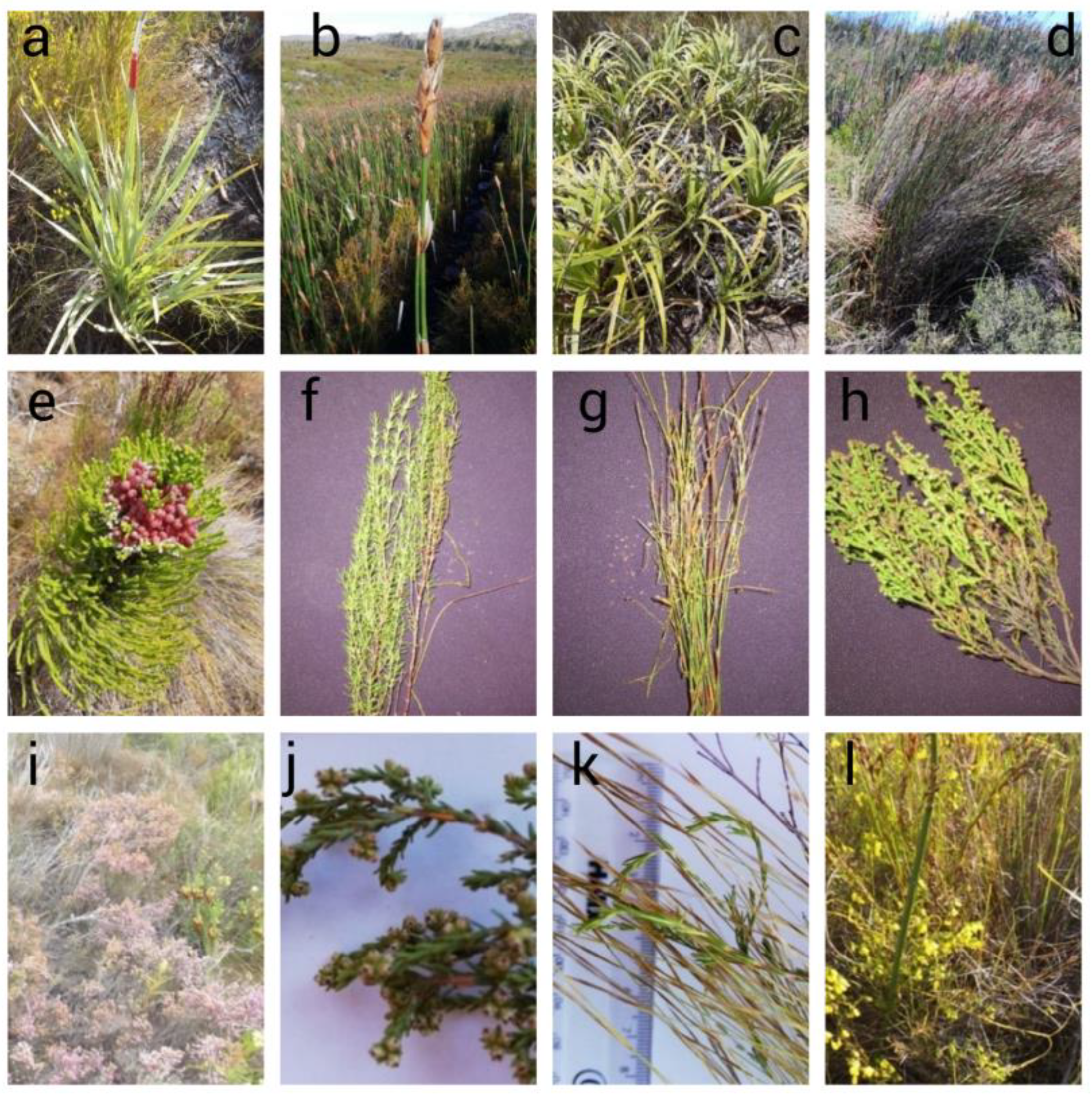
Eleven spatially dominant wetland plant species comprising several fynbos families were identified by traversing the wetland along transect lines with a botanist (see Figure 2). Table 1 summarizes key plant traits of the dominant species.
Elegia mucronata and Platycaulos compressus (Restioaceae) are tall, tufted restios found in moist soils. Their tall clusters and dark flowers are easily identifiable in aerial photos, while Restio dispar and Restio leptostachyus, also belonging to this family, occupy waterlogged zones. The former features red tufts that stand out in aerial images. Berzelia lanuginosa (Bruniaceae) is distinguished by its cottony, radiating flowerheads. Bobartia gladiata (Iridaceae), a yellow-flowering geophyte, is typically associated with post-fire recovery. The striking colours of the flowers in both species are important for their identification in aerial photography. The Erica species—E. serrata, E. intervallaris, and E. campanularis (Ericaceae)—occur on the drier peripheries, with small brown, pink, and yellow flowers, respectively. However, their small size and canopy make them less distinguishable than other species. Grubbia rosmarinifolia (Grubbiaceae), a shrub with narrow, rosemary-like leaves, is restricted to very waterlogged soils, while Tetraria thermalis (Cyperaceae), a non-wetland pioneer sedge, is found on the drier western margins. Most species flower lower in spring. This diverse assemblage reflects the influence of hydrological gradients and microhabitat variation within the wetland system.

2.3. Reconnaisance and Acquisition of UAV Data

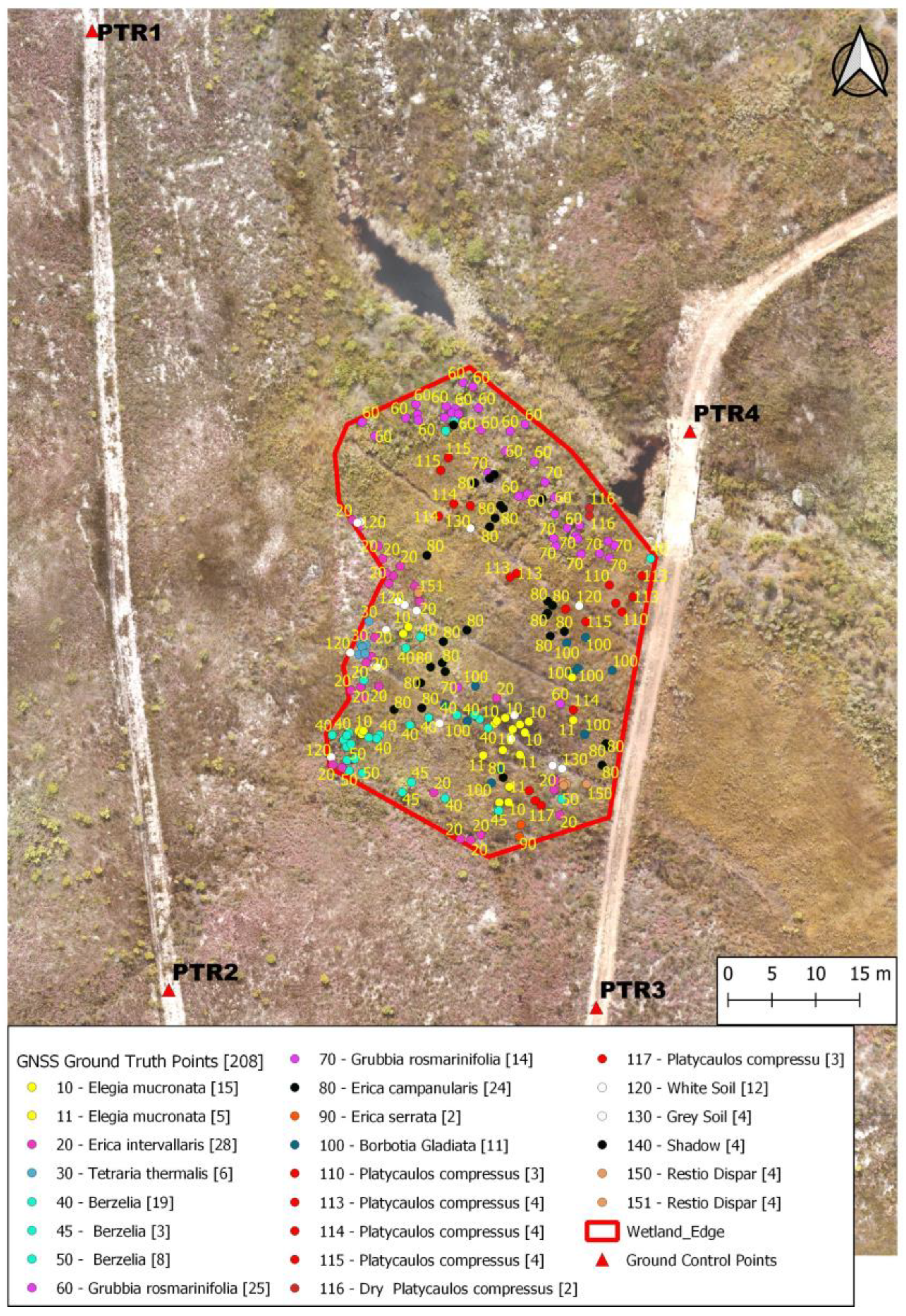
Ground control points were placed on site before the acquisition of aerial photography to ensure high positional and geometric accuracy in the processed orthomosaics. Five Ground Control Points (GCPs) points were surveyed around the edges of the study area (Figure 3).
An additional 211 ground truth points and their corresponding land cover per point were also surveyed within the wetland as ground truthing data. The sampling was mainly based on Stratified Proportional Random Sampling (SPRS) [57,58]. The wetland was divided into strata according to plant species distribution zones, with more intensive sampling in larger or more diverse strata, that is, areas with high species diversity. The SPRS approach aimed to improve classification accuracy by ensuring each vegetation type was represented correctly, enhancing the overall mapping and monitoring of species. Based on the points, 257 polygons were digitized in a GIS environment to correspond with the points.
A Parrot Sequoia camera (AgEagle Aerial Systems, Wichita, KS, USA) mounted on a DJI Phantom 3 quadcopter, and a MicaSense RedEdge-M camera (AgEagle Aerial Systems, Wichita, KS, USA) mounted on a DJI Phantom 4 Professional (DJI, Shenzhen, China) were used for image capture. The flights were conducted at an altitude of 25 m above ground level, with 80% forward and side overlap and a flight speed of 5 m/s. This low flying altitude helped capture detailed imagery while minimizing atmospheric distortion. However, the flight was high enough so as not to disturb the vegetation through propeller downdraft. The high degree of overlap also ensured that each GCP appeared in multiple images, enhancing georeferencing accuracy.
The Parrot Sequoia and MicaSense RedEdge-M sensors were calibrated using a calibration panel and irradiance sensors, respectively. The specific spectral bands for both sensors are detailed in Table 2 and Table 3. Flight dates, times, and corresponding seasons are summarized in Table 4.

2.4. Processing UAV Data

The data processing was performed in Pix4Dmapper version 4.4.12 (Pix4D SA, Lausanne, Switzerland). The first step in processing UAV data involved geometric calibration to correct distortions caused by factors such as lens and sensor misalignment, as well as terrain variation. These distortions can affect spatial accuracy, leading to pixel mismatches and image blur. To address this, the study employed a self-calibration bundle block adjustment based on image data, structure from motion (SfM), and ground control points (GCPs) surveyed using GNSS. The camera pose was established using metadata and updated in the aerial triangulation process. The resulting sparse point cloud was georeferenced to the South African Hartebeesthoek94 coordinate system, and elevations were constrained to SAGEOID 2010. This process facilitated the generation of high-resolution orthomosaics (1–3 cm) and a Digital Surface Model (DSM).
The second step was radiometric correction to convert raw UAV data into at-surface reflectance values. Radiometric correction was also done using Pix4Dmapper version 4.4.12 (Pix4D SA, Lausanne, Switzerland). For MicaSense RedEdge data, reflectance was calculated using irradiance metadata, while for Parrot Sequoia, reflectance was derived from pre- and post-flight calibration panel photos. The targetless approach relies on irradiance sensors to measure in situ solar irradiance mid-flight, as well as the omega, phi, and kappa flight orientation angles to calculate at-surface reflectance by dividing camera radiance by sensor irradiance [59,60]. Due to the brevity of UAV flights, the effects of variability in solar altitude, azimuth angles, and solar radiation during data capture on small sites are often considered negligible [61]. In the calibration panel approach, an empirical line regression was calculated between the digital numbers of the reflectance panels and their known reflectance and used to convert the digital numbers in the photographs to at-surface reflectance [62,63]. Overall, the study’s radiometric correction methods were consistent with those used in previous UAV-based research and produced comparable results.

2.5. Creating Spectral Indices

Vegetation indices are typically calculated between bands with the most significant variance in reflectance, i.e., those highly absorbed and those highly reflected by vegetation [64]. The choice of bands depends on the environmental and biophysical characteristics being investigated, such as leaf pigment content, biomass, moisture content, leaf structure and soil moisture [65,66,67,68]. This study utilized multispectral band orthomosaics to calculate indices in Pix4Dmapper version 4.4.12 (Pix4D SA, Lausanne, Switzerland), corresponding to several environmental and biophysical characteristics. The indices calculated were NGRDI [69], NDRE [70], CIRE [71], RG [15], Log Red [15], and Log Red Edge [15], which were selected because they had been highlighted in previous research [15] for their effectiveness in discriminating fynbos wetland species. Their efficacy stems from their sensitivity to leaf pigments (mainly chlorophyll and anthocyanins), leaf area, biomass, and canopy water content among the plant species. The indices were layer stacked with the captured spectral bands prior to feature selection and classification.

2.6. Classification of the Wetland Species

Geographic object-based image analysis (GEOBIA) classification techniques are increasingly being used in remote sensing studies. However, identifying the ideal segmentation criteria is often based on trial and error, which can sometimes lead to the identification of numerous and conflicting criteria, under-segmentation and over-segmentation [71,72]. Moreover, the segmentation process is sensitive to changes in radiometric conditions; thus, the transferability of the segmentation and classification parameters between different scenes is poor [73]. Considering these challenges, despite the increasing popularity of GEOBIA, Pixel-based (PB) classification approaches are still very popular in wetland studies [5,74,75]. Further, studies have compared the accuracy of GEOBIA and PB methods with conflicting results. Some found the GEOBIA approach gave better results [76,77,78], and others recommended the PB approach [79,80,81,82]. Consequently, this study used a PB approach with a Random Forest classifier (RF).
RF is an ensemble learning algorithm that builds several decision trees and combines their results to improve classification accuracy [83]. One of the central hyperparameters of Random Forest is ‘mtry’, which defines the number of randomly drawn candidate variables considered at each split when growing a tree; lower values lead to more diverse, less correlated trees and thus greater stability when aggregating. Another key parameter is the number of trees (ntree), which controls how reliable and stable the aggregated predictions are because too few trees result in instability. Conversely, too many add unnecessary computation [84].
The dataset consisted of the multispectral bands and calculated indices. In the latter, the dimensionality of the data was reduced by feature selection using recursive feature elimination (RFE) in R software (version 4.3.1) using ‘Caret’ and ‘Random Forest’ libraries. RFE iteratively trains a classification model, starting with all features and discarding the lowest-ranking features based on their contribution to the model’s performance [85]. The top ten features were layer-stacked for the classification of wetland species using Quantum GIS (QGIS) software (version 3.40).
Ground truth data were used to train a Random Forest (RF) classifier, with 70% of the samples allocated for supervised classification. RF has been reported to perform well in mapping heterogeneous wetlands [86,87,88]. RF relies on the ‘collective wisdom of the crowd’ to identify the appropriate class of the feature of interest. During training, decision trees are created on randomly selected subsets of the training data and available features [89]. This technique, called bagging, reduces overfitting by increasing diversity among trees in the prediction [90,91,92]. RF aggregates the predictions of multiple independent decision trees to determine the final classification and overall robustness of the classification model [83,90]. Before classification, the optimal hyperparameters (‘ntree’ and ‘mtry’) were determined through an iterative grid search using the ‘Dzetsaka’ plugin in QGIS [93]. The use of feature selection and hyperparameter tuning is commonly recommended in land cover studies [94]. Finally, the classification accuracy was assessed using the residual 30% of the samples as a validation set, with accuracy metrics calculated via the ‘Semi-Automatic Classification Plugin (SCP)’ [95] version 8.5.0. The evaluation metrics included overall accuracy, the kappa coefficient, and class-specific producer and user accuracies.

2.7. Statistical Analysis

A Shapiro–Wilk and Levene’s test [96] were used to assess the normality and homogeneity of the classification results (kappa, user accuracy, and producer accuracy), respectively. Subsequently, since the PA, UA, and Kappa were not normally distributed, Kruskal–Wallis and Wilcoxon tests (with Bonferroni correction) [97] were performed, using seasons as the predictor variable and the classification results as the response variables, to verify the significance of accuracy differences between seasons and sensors. A direct comparison, without Bonferroni correction, was also made between late Summer 2019 and late summer 2020, where different sensors were used.
The methodology is summarized in Figure 4; however, a more detailed description of the GNSS survey, geometric and radiometric corrections is described in our previous publications [15,56].

3. Results and Discussion

This study sought to address two key gaps in the limited research on remote sensing of Fynbos wetlands. The first objective was to evaluate the influence of seasonal variation on the ability of UAV data to discriminate between wetland vegetation species. The second was to identify the most suitable time of year for achieving accurate species-level classification within these distinctive ecosystems.

3.1. Seasonal Classification Results

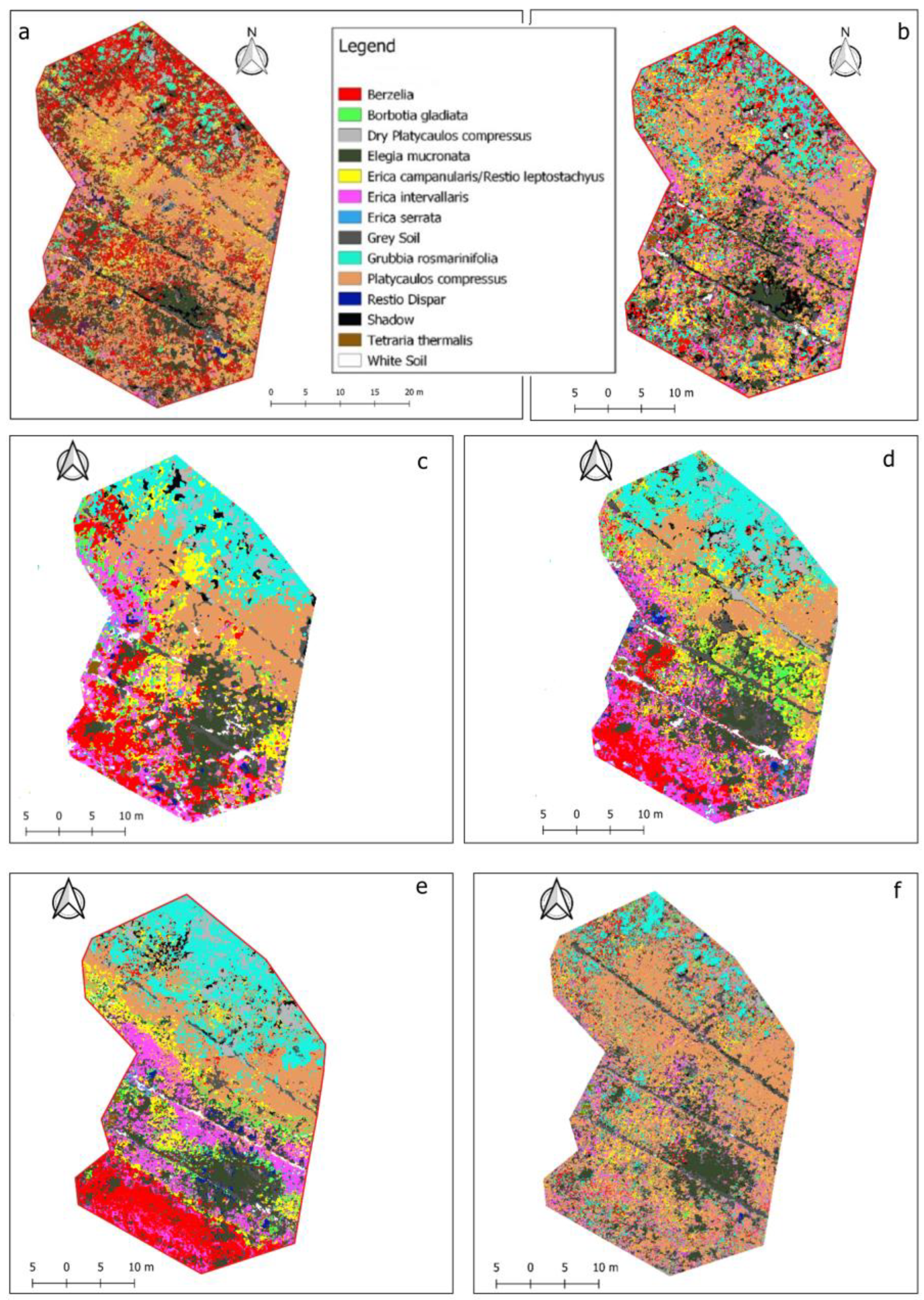
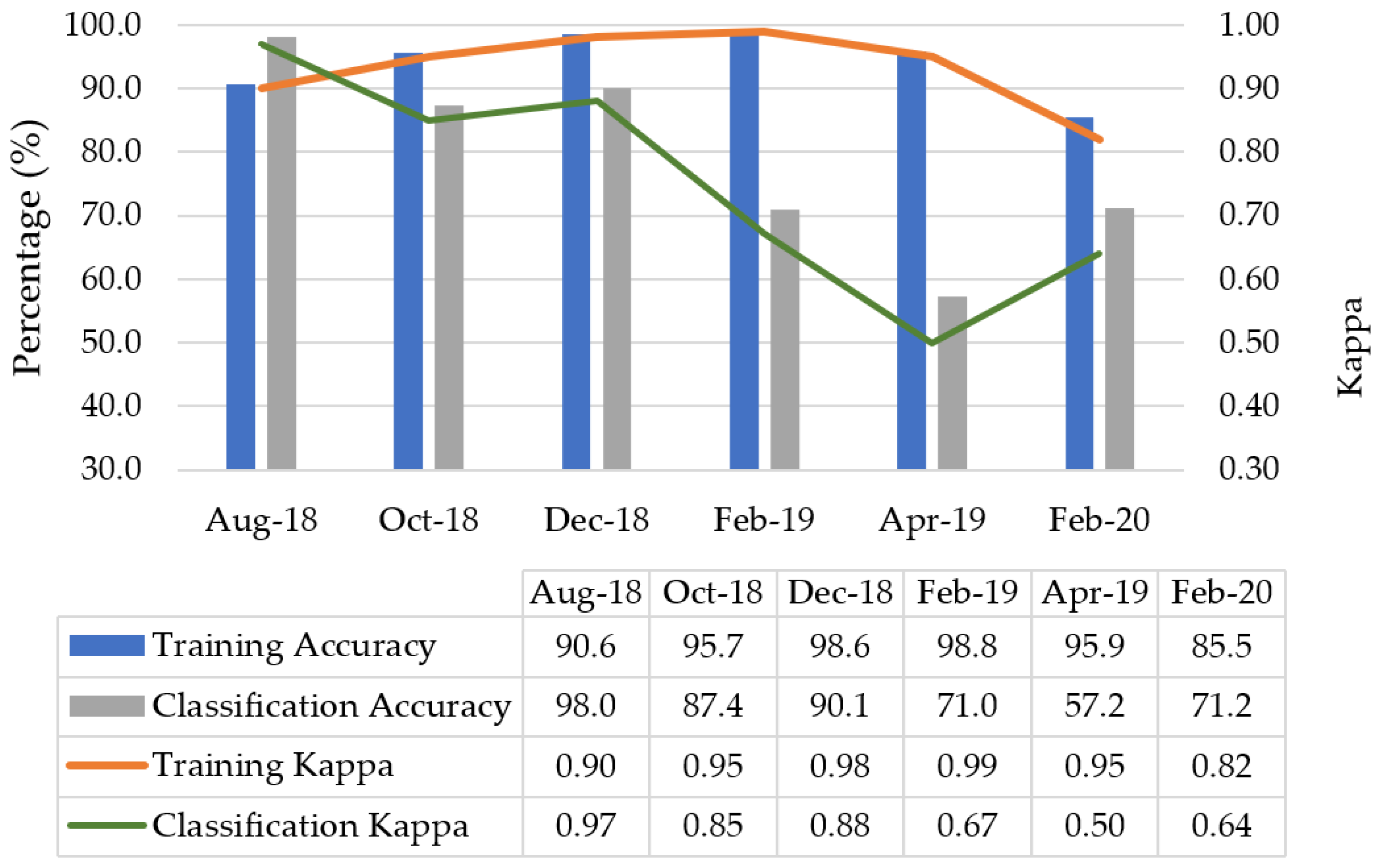
Figure 5 shows the classification maps, and Figure 6 shows the classification accuracies that were created for each of the seasons. The classification maps consistently show clusters of Elegia mucronata in the southwest of the wetland site. Platycaulos compressus was the most dominant wetland plant around the northernmost transect line. Similarly, Grubbia rosmarinifolia was also located in the northern part of the wetland, which is always inundated. The Ericicae species were consistently classified in the centre of the wetland along the second transect line in seasonally inundated soils. In general, Platycaulos compressus, Grubbia rosmarinifolia, Elegia mucronata, and Bobartia gladiata were the most stable classifications across seasons, occurring in both seasonal and permanently inundated areas of the wetland.
The classification training accuracies were generally high, ranging between 85.5% and 98.8% (Figure 6). The classification accuracy peaked in August 2018 (late winter), followed by December 2018 (early summer), and October 2018 (late spring).
The poorest overall accuracy was recorded in April 2019. There were similar classification accuracies in February 2019 and February 2020 (late summer). The results suggest that the optimal time for species discrimination occurs at the onset of the flowering season, marking the end of winter and the beginning of spring. However, the ideal time for the classification of specific species may vary across different seasons.

3.2. Temporal Insights into Species-Specific Classification Accuracy

Figure 7 shows the seasonal kappa values per class. The acronyms in the figure are: B (Berzelia), BG (Borbotia gladiata), DPC (Dry or Dead Platycaulos compressus), EM (Elegia mucronata), EC (Erica campanularis), EI (Erica intervallaris), ES (Erica serrata), GR (Grubbia rosmarinifolia), PC (Platycaulos compressus), RD (Restio Dispar), and TT (Tetraria thermalis).
The most consistently distinguishable species across the seasons were E. mucronata, G. rosmarinifolia, and P. compressus Additionally, T. thermalis was generally well classified across the seasons except for autumn 2019 (April) and summer 2020 (February). G. rosmarinifolia and P. compressus were located in the northern part of the wetland, which is the lowest-lying and consistently wet area. The persistent wetness in that part of the wetland may explain the spectral stability of the species throughout the different seasons.
Conversely, E. mucronata and T. thermalis were in the periodically inundated sections of the wetland; consequently, their spectral separability may be due to their better adaptation to seasonally fluctuating soil moisture in the seep wetland. Previous studies have shown that the diversity and reflectance spectra of wetlands are influenced by underlying water and moist soil. Table 5 provides a summary of the confusion matrices, emphasizing the classification accuracies of the species across different seasons. The complete confusion matrices have been included as Supplementary Materials.
The overall classification metric in August was 8% higher than the next best classification from December 2018. Apart from Tetraria thermalis, the producer accuracy of the plant species ranged from 75.4% to 100%, indicating that the random forest classification model could adequately fit the training data for most plant species. Furthermore, the user accuracies ranged from 83.3% to 100%, suggesting that the final classification maps generally reflect the actual locations of the plant species within the wetland. The lowest producer and user accuracies were attributed to Erica serrata. The results show that the model correctly predicted this class 83.3% of the time. However, it missed more than half of the actual instances, possibly due to within-class spectral variations.
The descriptions of the acronyms above are as follows: OA denotes Overall accuracy, PA denotes Producer Accuracy, UA denotes User Accuracy. B (Berzelia), BG (Borbotia gladiata), DPC (Dry or Dead Platycaulos compressus), EM (Elegia mucronata), EC (Erica campanularis), EI (Erica intervallaris), ES (Erica serrata), GR (Grubbia rosmarinifolia), PC (Platycaulos compressus), RD (Restio Dispar), and TT (Tetraria thermalis).
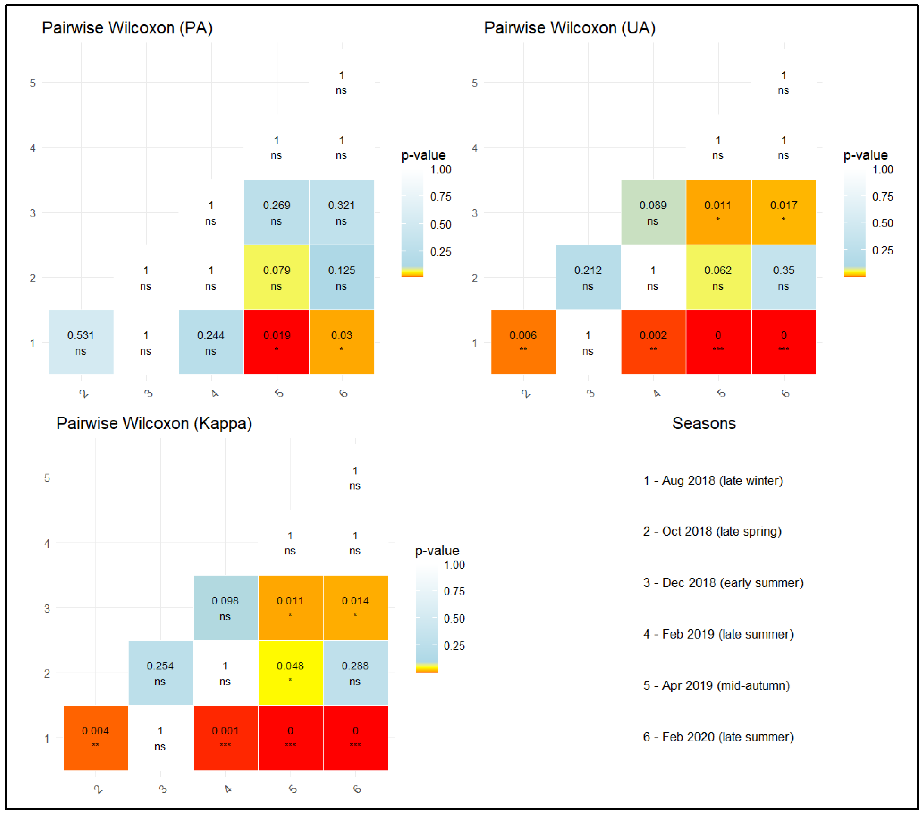
The Kruskal–Wallis test results for the cross-seasonal PA, UA and kappa were p = 0.000626, p = 0.00000106 and p = 0.000000651, respectively. The results (p-values < 0.05) confirm statistically significant differences in classification accuracies between seasons for all three metrics (PA, UA, and Kappa). Figure 8 presents the results of the pairwise Wilcoxon tests. Significant differences (p-values much lower than 0.05) were found between the user accuracies in the late winter season and those in all other seasons, except early summer.
Furthermore, there were significant differences in user accuracies between early summer and mid-autumn, as well as between early summer and late summer. Similar trends were observed for the Kappa accuracies. The significant differences for the producer accuracies were observed between late winter and mid-autumn, as well as between late winter and late summer.
These findings suggest that species discrimination is most effective at the onset of the flowering season, particularly during late winter and early spring, although optimal classification periods may differ among species.

3.3. Cross-Sensor Evaluation of Seasonal Species Classification Accuracy

The aerial photographs were captured in February 2019 and February 2020 using a Parrot Sequoia and a MicaSense RedEdge-M sensor, respectively. A comparison of the classification results across the two dates reveals similar trends in the classification of the species, except for E. serrata, R. dispar, and T. thermalis (see Figure 7, Table 5 and Figure 9).
The significance of the differences in accuracy was assessed using the Kruskal–Wallis test. The results showed p-values of 1.00 for PA, UA and Kappa metrics (Figure 8). The direct comparison (Wilcoxon rank-sum test) showed that the unadjusted p-values between both summer dates were 0.300, 0.439, 0.478 for PA, UA and Kappa, respectively. Both tests show that across all three metrics (PA, UA, Kappa), the two late summer classifications do not differ significantly, meaning the classification performance in February 2019 and February 2020 is statistically equivalent.
Consequently, the variance in classification accuracy may be due to changing conditions in the wetland such as soil moisture as opposed to sensor differences. Seasonal changes in plant phenology, such as flowering and senescence, or variations in environmental conditions, can significantly impact spectral reflectance and are inherently challenging to model.

3.4. Optimizing Remote Sensing Data Collection in CFR Seep Wetlands

Several satellite-based studies have demonstrated that classification accuracy can be improved by using data from multiple seasons. For example, Jenačković et al. [98] studied 185 permanent wetland vegetation plots with eleven plant communities across several seasons in the central Balkan Peninsula, showing that summer was optimal for identifying most species in hydrologically stable habitats, whereas spring was more appropriate for periodically inundated habitats. Similarly, Piaser & Villa [99] tested several combinations of feature dates across European lakes and found the highest accuracies when classifying aquatic vegetation using July–August datasets. Van Deventer et al. [55] found that combing four seasons of RapidEye Imagery improved the classification accuracy of wetland and dryland vegetation communities in iSimangaliso Wetland Park in South Africa by 6%. These studies all highlight the benefits of combining multi-seasonal data.
Other studies, however, have focused on a single year of seasonal data to identify optimal classification windows. Rupasinghe & Chow-Fraser [100], using one year of Landsat 7, Landsat 8, and Sentinel-2 data, demonstrated that late summer and fall were the most effective periods for distinguishing invasive Phragmites australis from other wetland species in Canadian Lake Erie wetlands. Similarly, Dong et al. [101] tracked the spread of Spartina alterniflora in mangrove forests in China using Sentinel-1 SAR and Sentinel-2 multispectral data. They observed spectral similarity among wetland species but concluded that January and August were the best months for classification, achieving accuracies up to 99.63%.
Unlike satellite sensors, where spatial resolution is relatively coarse, UAV data provides very high spatial detail. While this is advantageous for fine-scale vegetation mapping, it makes the integration of multitemporal datasets technically challenging. For this reason, we adopted an approach of assessing each season separately rather than combining them. This strategy not only leverages the spatial strengths of UAV data but also allows phenological differences across seasons to be fully explored. The findings from this approach can inform future conservation and monitoring initiatives in the Cape Floristic Region (CFR), where understanding seasonal dynamics is critical for effective wetland management.

4. Conclusions

4.1. Seasonal Classification Results

The classification results demonstrated high training accuracies across all seasons, with the highest overall accuracy achieved in late winter (August 2018) and early summer (December 2018). Classification performance declined toward mid-autumn, with the lowest accuracy recorded in April 2019. Notably, similar levels of accuracy were observed in late summer seasons (February 2019 and February 2020). These findings suggest that conservation agencies and future research should prioritize remote sensing data collection at the end of winter or early summer to capitalize on phenological differences between plant species.

4.2. Temporal Insights into Species-Specific Classification Accuracy

The Elegia mucronata, Grubbia rosmarinifolia, and Platycaulos compressus were the most consistently classified species. The spectral stability of G. rosmarinifolia and P. compressus may be attributed to their occurrence in the permanently wet northern zone of the wetland. In contrast, the reliable classification of E. mucronata and T. thermalis, which occur in seasonally inundated areas, may reflect their adaptation to fluctuating moisture conditions. These findings support previous research linking wetland vegetation reflectance to soil moisture dynamics and highlight the importance of seasonal timing in species-level wetland classification.

4.3. Cross-Sensor Evaluation of Seasonal Species Classification Accuracy

The classification results across these two summer dates and different sensors (Parrot Sequoia and a MicaSense RedEdge-M) revealed broadly similar trends. This suggests that the observed variance in classification accuracy may be more driven by changes in wetland conditions, such as soil moisture, rather than by differences between sensors. Future studies should incorporate additional ground-truth data and sensors to better account for confounding environmental factors.

4.4. Future Work: Leveraging Emerging Technologies for Improved Wetland Vegetation Mapping

A promising future research trajectory for fynbos wetland monitoring lies in the integration of emerging digital technologies, particularly Artificial Intelligence (AI), Big Data, and the Internet of Things (IoT) [102]. AI can enhance species classification, predict ecological dynamics, and refine conservation strategies with greater precision. Big Data analytics provide the capacity to manage and analyze diverse datasets from remote sensing platforms, in situ measurements, and citizen science initiatives, enabling the detection of complex ecological patterns [103]. Additionally, IoT-enabled sensor networks can facilitate continuous data collection on hydrological processes, vegetation dynamics, and environmental stressors, supporting adaptive management responses [104]. Together, these technologies can establish a data-driven framework that enhances the accuracy, scalability, and temporal resolution of fynbos wetland monitoring, ultimately contributing to more effective conservation in the Cape Floristic Region.
As a further research direction, the BioSCape project [4,105,106] provides an important opportunity: its large-scale multi-sensor data acquisitions in October and November 2023 across the Greater Cape Floristic Region (GCFR) coincide with the seasonal windows identified in this study as optimal for classification. Leveraging BioSCape data to map wetlands, particularly where vegetation clusters are large and relatively homogeneous, holds great promise for improving our understanding of the phenological traits of endemic species in the CFR.

Supplementary Materials

The following supporting information can be downloaded at: https://www.mdpi.com/article/10.3390/geographies5040060/s1, Table S1: Seasonal confusion matrices.

Author Contributions

Conceptualization, K.M.; methodology, K.M., M.S. and J.S.; software, K.M.; validation, K.M.; formal analysis, K.M.; investigation, K.M.; resources, K.M., M.S. and J.S.; data curation, K.M.; writing—original draft preparation, K.M.; writing—review and editing, K.M., M.S. and J.S.; visualization, K.M.; supervision, M.S. and J.S.; project administration, M.S. and J.S. All authors have read and agreed to the published version of the manuscript.

Funding

The study was supported by the Cape Peninsula University of Technology Staff Development Programme.

Data Availability Statement

The datasets presented in this article are not readily available because the datasets are part of an ongoing study. Requests to access the datasets should be directed to the corresponding author.

Acknowledgments

We are thankful to the botanists who assisted with identifying the plant species in the field. We are also grateful to the UCT Biological Sciences Department and Drone Solutions International, who supported the data collection in this study. We are also thankful to the anonymous reviewers who assessed our paper.

Conflicts of Interest

The authors declare no conflicts of interest.

References

  1. Esterhuizen, N.; Forrester, J.; Esler, K.J.; Wigley-Coetzee, C.; Morcillo, R.J.; Kleinert, A.; Pérez-Fernández, M.; Valentine, A.J. Nitrogen and Phosphorus Influence Acacia Saligna Invasiveness in the Fynbos Biome. Plant Ecol. 2020, 221, 309–320. [Google Scholar] [CrossRef]
  2. Kraaij, T.; Baard, J.A.; Rikhotso, D.R.; Cole, N.S.; Van Wilgen, B.W. Assessing the Effectiveness of Invasive Alien Plant Management in a Large Fynbos Protected Area. Bothalia 2017, 47, a2105. [Google Scholar] [CrossRef]
  3. Hall, S.A.; Bastos, R.; Vicente, J.; Vaz, A.S.; Honrado, J.P.; Holmes, P.M.; Gaertner, M.; Esler, K.J.; Cabral, J.A. A Dynamic Modeling Tool to Anticipate the Effectiveness of Invasive Plant Control and Restoration Recovery Trajectories in South African Fynbos. Restor. Ecol. 2021, 29, e13324. [Google Scholar] [CrossRef]
  4. Cardoso, A.W.; Brodrick, P.G.; Wilson, A.M.; Slingsby, J.A.; Forbes, C.J.; Thornton, M.; Hestir, E.L. Increasing Data Access in Multi-Sensor Airborne Campaigns: Lessons from BioSCape in South Africa. In Proceedings of the IGARSS 2024—2024 IEEE International Geoscience and Remote Sensing Symposium, Athens, Greece, 7–12 July 2024; pp. 2898–2901. [Google Scholar]
  5. Thamaga, K.H.; Dube, T.; Shoko, C. Evaluating the Impact of Land Use and Land Cover Change on Unprotected Wetland Ecosystems in the Arid-Tropical Areas of South Africa Using the Landsat Dataset and Support Vector Machine. Geocarto Int. 2022, 37, 10344–10365. [Google Scholar] [CrossRef]
  6. Xulu, S.; Mbatha, N.; Peerbhay, K. Burned Area Mapping over the Southern Cape Forestry Region, South Africa Using Sentinel Data within GEE Cloud Platform. ISPRS Int. J. Geoinf. 2021, 10, 511. [Google Scholar] [CrossRef]
  7. van Blerk, J.J.; West, A.G.; Smit, J.; Altwegg, R.; Hoffman, M.T. UAVs Improve Detection of Seasonal Growth Responses During Post-Fire Shrubland Recovery. Landsc. Ecol. 2022, 37, 3179–3199. [Google Scholar] [CrossRef]
  8. Jovanovic, N.; Garcia, C.L.; Bugan, R.D.H.; Teich, I.; Rodriguez, C.M.G. Validation of Remotely-Sensed Evapotranspiration and NDWI Using Ground Measurements at Riverlands, South Africa. Water SA 2014, 40, 211–220. [Google Scholar] [CrossRef]
  9. Skowno, A.L.; Jewitt, D.; Slingsby, J.A. Rates and Patterns of Habitat Loss across South Africa’s Vegetation Biomes. S. Afr. J. Sci. 2021, 117, 1–6. [Google Scholar] [CrossRef]
  10. Chiloane, C.; Dube, T.; Shoko, C. Multispectral Remote Sensing of Potential Groundwater Dependent Vegetation in the Greater Floristic Region of the Western Cape, South Africa. S. Afr. Geogr. J. 2023, 105, 481–499. [Google Scholar] [CrossRef]
  11. Duncan, P.; Podest, E.; Esler, K.J.; Geerts, S.; Lyons, C. Mapping Invasive Herbaceous Plant Species with Sentinel-2 Satellite Imagery: Echium Plantagineum in a Mediterranean Shrubland as a Case Study. Geomatics 2023, 3, 328–344. [Google Scholar] [CrossRef]
  12. Slingsby, J.A.; Wilson, A.M.; Maitner, B.; Moncrieff, G.R. Regional Ecological Forecasting across Scales: A Manifesto for a Biodiversity Hotspot. Methods Ecol. Evol. 2023, 14, 757–770. [Google Scholar] [CrossRef]
  13. van Blerk, J.J.; Slingsby, J.A.; West, A.G. Unpacking Satellite Pixels: UAVs Reveal Fine-Scale Drivers of Land Surface Phenology in a Winter Rainfall Shrubland. Environ. Res. Lett. 2024, 19, 084008. [Google Scholar] [CrossRef]
  14. van Deventer, H.; Naidoo, L.; Apleni, P.; le Roux, J.; Blaauw, C.; Nel, W.; Tema, H. Remote Sensing Monitoring of Soil Moisture for South African. Water Wheel 2025, 24, 28–31. [Google Scholar]
  15. Musungu, K.; Dube, T.; Smit, J.; Shoko, M. Using UAV Multispectral Photography to Discriminate Plant Species in a Seep Wetland of the Fynbos Biome. Wetl. Ecol. Manag. 2024, 32, 207–227. [Google Scholar] [CrossRef]
  16. Walmsley, R. A Description of the Wetlands Research Programme; Foundation for Research Development: Pretoria, South Africa, 1988; Volume 145. [Google Scholar]
  17. Liu, H.; Liao, T.; Wang, Y.; Qian, X.; Liu, X.; Li, C.; Li, S.; Guan, Z.; Zhu, L.; Zhou, X.; et al. Fine-Grained Wetland Classification for National Wetland Reserves Using Multi-Source Remote Sensing Data and Pixel Information Expert Engine (PIE-Engine). GIsci. Remote Sens. 2023, 60, 2286746. [Google Scholar] [CrossRef]
  18. McDonald, A.; Gillespie, J. Beyond the Selective Regulation of Wetlands: Towards a Rights of Wetlands. Aust. Geogr. 2024, 55, 329–344. [Google Scholar] [CrossRef]
  19. Grenfell, M.C.; Abrahams, E.; Fisher, R.-M. Analysis and Conceptual Geospatial Modelling of the Intermediary Role of Wetlands in Drylands in Post-Fire Material Flux Dynamics, Silvermine River Catchment, Cape Town. Wetl. Ecol. Manag. 2022, 30, 623–645. [Google Scholar] [CrossRef]
  20. van Blerk, J.J.; Cramer, M.D.; West, A.G.; Musker, S.D.; Verboom, G.A. The Contribution of Hydric Habitats to the Richness of the Cape Fynbos Flora. Divers. Distrib. 2025, 31, e13962. [Google Scholar] [CrossRef]
  21. Chi, J.; Afandi, S.H.M.; Matthew, N.K.A. Mapping Hotspots and Emerging Trends in Global Wetlands Research: A Scientometric Analysis (2002–2022). J. Environ. Earth Sci. 2025, 7, 101–116. [Google Scholar] [CrossRef]
  22. He, Q.; Zhang, Z.; Zhang, Y.; Sun, T.; Wang, W.; Zhang, Z. Spatiotemporal Evolution and Driving Mechanisms of Ecological Risk in the Yuncheng Salt Lake Wetland, China. Water 2025, 17, 524. [Google Scholar] [CrossRef]
  23. Kaiss, R.; Benjouid, Z.; Snoussi, N.; El Mountassir, E.K.; Nabil, N.; Halim, A.; Zarouali, S.S. Impact of Climate Change on Water Resources and Ecological Sustainability in Morocco: A 1990–2022 Analysis. Res. Ecol. 2025, 7, 53–70. [Google Scholar] [CrossRef]
  24. Sadiki, M.; van Deventer, H.; Hansen, C. Assessing the Extent to Which African Wetland Inventories Can Report to the Global Targets on Biodiversity, Including Goal A of the Global Biodiversity Framework. Afr. J. Aquat. Sci. 2024, 49, 254–261. [Google Scholar] [CrossRef]
  25. Servat, G.P.; Alcocer, R.; Larico, M.V.; Olarte, M.E.; Linares-Palomino, R.; Alonso, A.; Ledesma, K. The Effects of Area and Habitat Heterogeneity on Bird Richness and Composition in High Elevation Wetlands (“Bofedales”) of the Central Andes of Peru. Wetlands 2018, 38, 1133–1145. [Google Scholar] [CrossRef]
  26. Stephenson, P.J.; Ntiamoa-Baidu, Y.; Simaika, J.P. The Use of Traditional and Modern Tools for Monitoring Wetlands Biodiversity in Africa: Challenges and Opportunities. Front. Environ. Sci. 2020, 8, 1–12. [Google Scholar] [CrossRef]
  27. Dube, T.; Musasa, T. Wetland Vegetation Species Diversity and Productivity Assessment: Implications on Ecosystem Services. In Revealing Ecosystem Services Through Geospatial Technologies; Mutanga, O., Pandey, P.C., Das, S., Chatterjee, U., Eds.; Spinger Nature: Cham, Switzerland, 2025; pp. 171–184. [Google Scholar]
  28. Faelga, R.A.; Assiri, M.; Silvestri, S. UAV Photogrammetry-Based Leaf Area Index for Above-Ground Biomass Estimation in Wetlands. IEEE J. Sel. Top Appl. Earth Obs. Remote Sens. 2025, 18, 13844–13861. [Google Scholar] [CrossRef]
  29. Hu, Q.; Zhang, L.; Drahota, J.; Woldt, W.; Varner, D.; Bishop, A.; LaGrange, T.; Neale, C.M.U.; Tang, Z. Combining Multi-View UAV Photogrammetry, Thermal Imaging, and Computer Vision Can Derive Cost-Effective Ecological Indicators for Habitat Assessment. Remote Sens. 2024, 16, 1081. [Google Scholar] [CrossRef]
  30. Fromm, L.T.; Smith, L.C.; Kyzivat, E.D. Wetland Vegetation Mapping Improved by Phenological Leveraging of Multitemporal Nanosatellite Images. Geocarto Int. 2025, 40, 2452252. [Google Scholar] [CrossRef]
  31. Hill, W.; Unwin, M.; Eckersley, S.; Bernadini, N.; Turconi, A.; Da Silva Curiel, A.; Cardellach, E.; Pirat, C. HydroSwarm: Using a Cooperative Swarm of CubeSats to Enhance GNSS-R Capabilities for Surface Soil Moisture and Inundation Measurements. In Proceedings of the Small Satellites Systems and Services Symposium (4S 2024), Palma de Mallorca, Spain, 27–31 May 2024; Petrozzi-Ilstad, M., Ed.; SPIE: Bellingham, WA, USA, 2025; p. 113. [Google Scholar]
  32. Alizadeh Moghaddam, S.H.; Gazor, S.; Homayouni, S.; Karami, F. Multiscale Deformable DenseNet for Wetland Mapping Using Hyperspectral Images. IEEE Geosci. Remote Sens. Lett. 2025, 22, 1–5. [Google Scholar] [CrossRef]
  33. Magidi, J.; Bangira, T.; Kelepile, M.; Shoko, M. Land Use and Land Cover Changes in Notwane Watershed, Botswana, Using Extreme Gradient Boost (XGBoost) Machine Learning Algorithm. Afr. Geogr. Rev. 2024, 44, 497–517. [Google Scholar] [CrossRef]
  34. Solórzano, J.V.; Peralta-Carreta, C.; Gallardo-Cruz, J.A. Mapping Tropical Forested Wetlands Biomass with LiDAR: A Machine Learning Comparison. Remote Sens. 2025, 17, 1076. [Google Scholar] [CrossRef]
  35. Paudel, A.; Richardson, M.; King, D. Multispectral and LiDAR-Derived Vegetation Indicators of Water Table Dynamics in Forested Wetlands. Can. J. Remote Sens. 2025, 51, 2471502. [Google Scholar] [CrossRef]
  36. Deng, Y.; Shi, R.; Zhang, C.; Wang, X.; Liu, C.; Gao, W. Wetland Vegetation Species Classification Using Optical and SAR Remote Sensing Images: A Case Study of Chongming Island, Shanghai, China. Chin. Geogr. Sci. 2025, 35, 510–527. [Google Scholar] [CrossRef]
  37. Varugu, B.K.; Jones, C.E.; Oliver-Cabrera, T.; Simard, M.; Jensen, D.J. Study of Hydrologic Connectivity and Tidal Influence on Water Flow Within Louisiana Coastal Wetlands Using Rapid-Repeat Interferometric Synthetic Aperture Radar. Remote Sens. 2025, 17, 459. [Google Scholar] [CrossRef]
  38. Taddeo, S.; Dronova, I.; Depsky, N. Spectral Vegetation Indices of Wetland Greenness: Responses to Vegetation Structure, Composition, and Spatial Distribution. Remote Sens. Environ. 2019, 234, 111467. [Google Scholar] [CrossRef]
  39. Miller, G.J.; Dronova, I.; Oikawa, P.Y.; Knox, S.H.; Windham-Myers, L.; Shahan, J.; Stuart-Haëntjens, E. The Potential of Satellite Remote Sensing Time Series to Uncover Wetland Phenology under Unique Challenges of Tidal Setting. Remote Sens. 2021, 13, 3589. [Google Scholar] [CrossRef]
  40. Borges, J.; Higginbottom, T.P.; Symeonakis, E.; Jones, M. Sentinel-1 and Sentinel-2 Data for Savannah Land Cover Mapping: Optimising the Combination of Sensors and Seasons. Remote Sens. 2020, 12, 3862. [Google Scholar] [CrossRef]
  41. Pargieła, K. Optimising UAV Data Acquisition and Processing for Photogrammetry: A Review. Geomat. Environ. Eng. 2023, 17, 29–59. [Google Scholar] [CrossRef]
  42. Surasinghe, T.D.; Singh, K.K.; Smart, L.S. Leveraging Phenology to Assess Seasonal Variations of Plant Communities for Mapping Dynamic Ecosystems. Remote Sens. 2025, 17, 1778. [Google Scholar] [CrossRef]
  43. Im, J.; Jensen, J.R. Hyperspectral Remote Sensing of Vegetation. Geogr. Compass 2008, 2, 1943–1961. [Google Scholar] [CrossRef]
  44. Conrad, C.; Dech, S.; Dubovyk, O.; Fritsch, S.; Klein, D.; Löw, F.; Schorcht, G.; Zeidler, J. Derivation of Temporal Windows for Accurate Crop Discrimination in Heterogeneous Croplands of Uzbekistan Using Multitemporal RapidEye Images. Comput. Electron. Agric. 2014, 103, 63–74. [Google Scholar] [CrossRef]
  45. Jönsson, P.; Cai, Z.; Melaas, E.; Friedl, M.; Eklundh, L. A Method for Robust Estimation of Vegetation Seasonality from Landsat and Sentinel-2 Time Series Data. Remote Sens. 2018, 10, 635. [Google Scholar] [CrossRef]
  46. Kang, X.; Hao, Y.; Cui, X.; Chen, H.; Huang, S.; Du, Y.; Li, W.; Kardol, P.; Xiao, X.; Cui, L. Variability and Changes in Climate, Phenology, and Gross Primary Production of an Alpine Wetland Ecosystem. Remote Sens. 2016, 8, 391. [Google Scholar] [CrossRef]
  47. Ai, J.; Gao, W.; Gao, Z.; Shi, R.; Zhang, C. Phenology-Based Spartina Alterniflora Mapping in Coastal Wetland of the Yangtze Estuary Using Time Series of GaoFen Satellite No. 1 Wide Field of View Imagery. J. Appl. Remote Sens. 2017, 11, 026020. [Google Scholar] [CrossRef]
  48. Fan, C.; Yang, J.; Zhao, G.; Dai, J.; Zhu, M.; Dong, J.; Liu, R.; Zhang, G. Mapping Phenology of Complicated Wetland Landscapes through Harmonizing Landsat and Sentinel-2 Imagery. Remote Sens. 2023, 15, 2413. [Google Scholar] [CrossRef]
  49. Larkin, D.J. Wetland Heterogeneity. In The Wetland Book; Springer: Dordrecht, The Netherlands, 2018; pp. 177–182. ISBN 9789048196593. [Google Scholar]
  50. Nhamo, L.; Magidi, J.; Dickens, C. Determining Wetland Spatial Extent and Seasonal Variations of the Inundated Area Using Multispectral Remote Sensing. Water SA 2017, 43, 543–552. [Google Scholar] [CrossRef]
  51. Torbick, N.; Salas, W. Mapping Agricultural Wetlands in the Sacramento Valley, USA with Satellite Remote Sensing. Wetl. Ecol. Manag. 2015, 23, 79–94. [Google Scholar] [CrossRef]
  52. Dronova, I.; Taddeo, S.; Harris, K. Plant Diversity Reduces Satellite-Observed Phenological Variability in Wetlands at a National Scale. Sci. Adv. 2022, 8, 8214. [Google Scholar] [CrossRef]
  53. Kovács, G.M.; Horion, S.; Fensholt, R. Characterizing Ecosystem Change in Wetlands Using Dense Earth Observation Time Series. Remote Sens. Environ. 2022, 281, 113267. [Google Scholar] [CrossRef]
  54. Van Deventer, H. Remote Sensing of Wetland Tree Species in the ISimangaliso Wetland Park, KwaZulu-Natal, South Africa; University of KwaZulu-Natal: Pietermaritzburg, South Africa, 2016. [Google Scholar]
  55. van Deventer, H.; Cho, M.A.; Mutanga, O. Multi-Season RapidEye Imagery Improves the Classification of Wetland and Dryland Communities in a Subtropical Coastal Region. ISPRS J. Photogramm. Remote Sens. 2019, 157, 171–187. [Google Scholar] [CrossRef]
  56. Musungu, K.; Shoko, M.; Smit, J. Determining the Spectral Characteristics of Fynbos Wetland Vegetation Species Using Unmanned Aerial Vehicle Data. Geomatics 2025, 5, 17. [Google Scholar] [CrossRef]
  57. Mu, X.; Hu, M.; Song, W.; Ruan, G.; Ge, Y.; Wang, J.; Huang, S.; Yan, G. Evaluation of Sampling Methods for Validation of Remotely Sensed Fractional Vegetation Cover. Remote Sens. 2015, 7, 16164–16182. [Google Scholar] [CrossRef]
  58. Shetty, S.; Gupta, P.K.; Belgiu, M.; Srivastav, S.K. Assessing the Effect of Training Sampling Design on the Performance of Machine Learning Classifiers for Land Cover Mapping Using Multi-Temporal Remote Sensing Data and Google Earth Engine. Remote Sens. 2021, 13, 1433. [Google Scholar] [CrossRef]
  59. Cao, S.; Danielson, B.; Clare, S.; Koenig, S.; Campos-Vargas, C.; Sanchez-Azofeifa, A. Radiometric Calibration Assessments for UAS-Borne Multispectral Cameras: Laboratory and Field Protocols. ISPRS J. Photogramm. Remote Sens. 2019, 149, 132–145. [Google Scholar] [CrossRef]
  60. Daniels, L.; Eeckhout, E.; Wieme, J.; Dejaegher, Y.; Audenaert, K.; Maes, W.H. Identifying the Optimal Radiometric Calibration Method for UAV-Based Multispectral Imaging. Remote Sens. 2023, 15, 2909. [Google Scholar] [CrossRef]
  61. Guo, Y.; Senthilnath, J.; Wu, W.; Zhang, X.; Zeng, Z.; Huang, H. Radiometric Calibration for Multispectral Camera of Different Imaging Conditions Mounted on a UAV Platform. Sustainability 2019, 11, 978. [Google Scholar] [CrossRef]
  62. Tmušić, G.; Manfreda, S.; Aasen, H.; James, M.R.; Gonçalves, G.; Ben-Dor, E.; Brook, A.; Polinova, M.; Arranz, J.J.; Mészáros, J.; et al. Current Practices in UAS-Based Environmental Monitoring. Remote Sens. 2020, 12, 1001. [Google Scholar] [CrossRef]
  63. Zhu, H.; Huang, Y.; An, Z.; Zhang, H.; Han, Y.; Zhao, Z.; Li, F.; Zhang, C.; Hou, C. Assessing Radiometric Calibration Methods for Multispectral UAV Imagery and the Influence of Illumination, Flight Altitude and Flight Time on Reflectance, Vegetation Index and Inversion of Winter Wheat AGB and LAI. Comput. Electron. Agric. 2024, 219, 108821. [Google Scholar] [CrossRef]
  64. Solymosi, K.; Kövér, G.; Romvári, R. The Progression of Vegetation Indices: A Short Overview. Acta Agrar. Kaposváriensis 2019, 23, 75–90. [Google Scholar] [CrossRef]
  65. Xue, J.; Su, B. Significant Remote Sensing Vegetation Indices: A Review of Developments and Applications. J. Sens. 2017, 2017, 1353691. [Google Scholar] [CrossRef]
  66. Bhagat, V.; Kada, A.; Kumar, S. Analysis of Remote Sensing Based Vegetation Indices (VIs) for Unmanned Aerial System (UAS): A Review. Remote Sens. Land 2020, 3, 58–73. [Google Scholar] [CrossRef]
  67. Giovos, R.; Tassopoulos, D.; Kalivas, D.; Lougkos, N.; Priovolou, A. Remote Sensing Vegetation Indices in Viticulture: A Critical Review. Agriculture 2021, 11, 457. [Google Scholar] [CrossRef]
  68. Ma, S.; Zhou, Y.; Gowda, P.H.; Dong, J.; Zhang, G.; Kakani, V.G.; Wagle, P.; Chen, L.; Flynn, K.C.; Jiang, W. Application of the Water-Related Spectral Reflectance Indices: A Review. Ecol. Indic. 2019, 98, 68–79. [Google Scholar] [CrossRef]
  69. Poley, L.; McDermid, G. A Systematic Review of the Factors Influencing the Estimation of Vegetation Aboveground Biomass Using Unmanned Aerial Systems. Remote Sens. 2020, 12, 1052. [Google Scholar] [CrossRef]
  70. Walsh, O.S.; Shafian, S.; Marshall, J.M.; Jackson, C.; McClintick-Chess, J.R.; Blanscet, S.M.; Swoboda, K.; Thompson, C.; Belmont, K.M.; Walsh, W.L. Assessment of UAV Based Vegetation Indices for Nitrogen Concentration Estimation in Spring Wheat. Adv. Remote Sens. 2018, 7, 71–90. [Google Scholar] [CrossRef]
  71. Guirado, E.; Tabik, S.; Alcaraz-Segura, D.; Cabello, J.; Herrera, F. Deep-Learning Versus OBIA for Scattered Shrub Detection with Google Earth Imagery: Ziziphus Lotus as Case Study. Remote Sens. 2017, 9, 1220. [Google Scholar] [CrossRef]
  72. Dronova, I. Object-Based Image Analysis in Wetland Research: A Review. Remote Sens. 2015, 7, 6380–6413. [Google Scholar] [CrossRef]
  73. Veljanovski, T.; Kanjir, U.; Oštir, K. Object-Based Image Analysis of Remote Sensing Data. Geod. Vestn. 2011, 55, 641–688. [Google Scholar] [CrossRef]
  74. Slagter, B.; Tsendbazar, N.E.; Vollrath, A.; Reiche, J. Mapping Wetland Characteristics Using Temporally Dense Sentinel-1 and Sentinel-2 Data: A Case Study in the St. Lucia Wetlands, South Africa. Int. J. Appl. Earth Obs. Geoinf. 2020, 86, 102009. [Google Scholar] [CrossRef]
  75. van Deventer, H.; Linström, A.; Naidoo, L.; Job, N.; Sieben, E.J.J.; Cho, M.A. Comparison between Sentinel-2 and WorldView-3 Sensors in Mapping Wetland Vegetation Communities of the Grassland Biome of South Africa, for Monitoring under Climate Change. Remote Sens. Appl. 2022, 28, 100875. [Google Scholar] [CrossRef]
  76. Zheng, J.Y.; Hao, Y.Y.; Wang, Y.C.; Zhou, S.Q.; Wu, W.B.; Yuan, Q.; Gao, Y.; Guo, H.Q.; Cai, X.X.; Zhao, B. Coastal Wetland Vegetation Classification Using Pixel-Based, Object-Based and Deep Learning Methods Based on RGB-UAV. Land 2022, 11, 2039. [Google Scholar] [CrossRef]
  77. Simioni, J.P.D.; Guasselli, L.A. Dual-Season Comparison of OBIA and Pixel-Based Approaches for Coastal Wetland Classification. Rev. Bras. Recur. Hidr. 2024, 29, e5. [Google Scholar] [CrossRef]
  78. Tonyaloğlu, E.E.; Erdoğan, N.; Çavdar, B.; Kurtşan, K.; Nurlu, E. Comparison of Pixel and Object Based Classification Methods on Rapideye Satellite Image. Turk. J. For. Sci. 2021, 5, 1–11. [Google Scholar] [CrossRef]
  79. Dervisoglu, A.; Bilgilioglu, B.B.; Yağmur, N. Comparison of Pixel-Based and Object-Based Classification Methods in Determination of Wetland Coastline. Int. J. Environ. Geoinform. 2020, 7, 213–220. [Google Scholar] [CrossRef]
  80. Islam, M.K.; Simic Milas, A.; Abeysinghe, T.; Tian, Q. Integrating UAV-Derived Information and WorldView-3 Imagery for Mapping Wetland Plants in the Old Woman Creek Estuary, USA. Remote Sens. 2023, 15, 1090. [Google Scholar] [CrossRef]
  81. Abeysinghe, T.; Simic Milas, A.; Arend, K.; Hohman, B.; Reil, P.; Gregory, A.; Vázquez-Ortega, A. Mapping Invasive Phragmites Australis in the Old Woman Creek Estuary Using UAV Remote Sensing and Machine Learning Classifiers. Remote Sens. 2019, 11, 1380. [Google Scholar] [CrossRef]
  82. De Giglio, M.; Greggio, N.; Goffo, F.; Merloni, N.; Dubbini, M.; Barbarella, M. Comparison of Pixel- and Object-Based Classification Methods of Unmanned Aerial Vehicle Data Applied to Coastal Dune Vegetation Communities: Casal Borsetti Case Study. Remote Sens. 2019, 11, 1416. [Google Scholar] [CrossRef]
  83. Breiman, L. Random Forests. Mach. Learn. 2001, 45, 5–32. [Google Scholar] [CrossRef]
  84. Probst, P.; Wright, M.N.; Boulesteix, A. Hyperparameters and Tuning Strategies for Random Forest. WIREs Data Min. Knowl. Discov. 2019, 9, e1301. [Google Scholar] [CrossRef]
  85. Speiser, J.L.; Miller, M.E.; Tooze, J.; Ip, E. A Comparison of Random Forest Variable Selection Methods for Classification Prediction Modeling. Expert Syst. Appl. 2019, 134, 93–101. [Google Scholar] [CrossRef]
  86. Berhane, T.M.; Costa, H.; Lane, C.R.; Anenkhonov, O.A.; Chepinoga, V.V.; Autrey, B.C. The Influence of Region of Interest Heterogeneity on Classification Accuracy in Wetland Systems. Remote Sens. 2019, 11, 551. [Google Scholar] [CrossRef]
  87. Deshambo, A.; Stewart, E.C.; Ulik, S.; Williams, J.M. Delineating Wetland Vegetation Species Using a UAV-Mounted Multi-Spectral Camera and Computer-Aided Classification. Proc. Wis. Space Conf. 2023, 1, 1. [Google Scholar] [CrossRef]
  88. Martínez Prentice, R.; Villoslada Peciña, M.; Ward, R.D.; Bergamo, T.F.; Joyce, C.B.; Sepp, K. Machine Learning Classification and Accuracy Assessment from High-Resolution Images of Coastal Wetlands. Remote Sens. 2021, 13, 3669. [Google Scholar] [CrossRef]
  89. Okolie, C.; Adeleke, A.; Mills, J.; Smit, J.; Maduako, I.; Bagheri, H.; Komar, T.; Wang, S. Assessment of Explainable Tree-Based Ensemble Algorithms for the Enhancement of Copernicus Digital Elevation Model in Agricultural Lands. Int. J. Image Data Fusion 2024, 15, 430–460. [Google Scholar] [CrossRef]
  90. Breiman, L. Bagging Predictors. Mach. Learn. 1996, 24, 123–140. [Google Scholar] [CrossRef]
  91. Eisavi, V.; Homayouni, S.; Yazdi, A.M.; Alimohammadi, A. Land Cover Mapping Based on Random Forest Classification of Multitemporal Spectral and Thermal Images. Environ. Monit. Assess 2015, 187, 291. [Google Scholar] [CrossRef]
  92. Ghasemian, N.; Akhoondzadeh, M. Introducing Two Random Forest Based Methods for Cloud Detection in Remote Sensing Images. Adv. Space Res. 2018, 62, 288–303. [Google Scholar] [CrossRef]
  93. Karasiak, N. Dzetsaka QGIS Classification Plugin 2016. Available online: https://github.com/nkarasiak/dzetsaka (accessed on 18 August 2025).
  94. Sovann, C.; Olin, S.; Mansourian, A.; Sakhoeun, S.; Prey, S.; Kok, S.; Tagesson, T. Importance of Spectral Information, Seasonality, and Topography on Land Cover Classification of Tropical Land Cover Mapping. Remote Sens. 2025, 17, 1551. [Google Scholar] [CrossRef]
  95. Congedo, L. Semi-Automatic Classification Plugin: A Python Tool for the Download and Processing of Remote Sensing Images in QGIS. J. Open Source Softw. 2021, 6, 3172. [Google Scholar] [CrossRef]
  96. Kim, S.; Lee, C.W.; Park, H.-J.; Hwang, J.E.; Park, H.B.; Yoon, Y.-J.; Kim, Y.-J. UAV Telephotography Elucidates Floristic Variability and Beta Diversity of Island Cliffs Under Grazing Interventions. Sci. Rep. 2024, 14, 15465. [Google Scholar] [CrossRef]
  97. Surasinghe, T.D.; Chen, Y.; Singh, K.K. Restored Wetlands Show Rapid Vegetation Recovery and Substantial Surface-water Expansion. Restor. Ecol. 2025, 33, e70046. [Google Scholar] [CrossRef]
  98. Jenačković, D.D.; Lakušić, D.; Zlatković, I.; Jušković, M.; Ranđelović, N.V. Emergent Wetland Vegetation Data Recording: Does an Optimal Period Exist? Appl. Veg. Sci. 2019, 22, 200–212. [Google Scholar] [CrossRef]
  99. Piaser, E.; Villa, P. Evaluating Capabilities of Machine Learning Algorithms for Aquatic Vegetation Classification in Temperate Wetlands Using Multi-Temporal Sentinel-2 Data. Int. J. Appl. Earth Obs. Geoinf. 2023, 117, 103202. [Google Scholar] [CrossRef]
  100. Rupasinghe, P.A.; Chow-Fraser, P. Identification of Most Spectrally Distinguishable Phenological Stage of Invasive Phramites Australis in Lake Erie Wetlands (Canada) for Accurate Mapping Using Multispectral Satellite Imagery. Wetl. Ecol. Manag. 2019, 27, 513–538. [Google Scholar] [CrossRef]
  101. Dong, D.; Wang, C.; Yan, J.; He, Q.; Zeng, J.; We, Z. Combing Sentinel-1 and Sentinel-2 Image Time Series for Invasive Spartina Alterniflora Mapping on Google Earth Engine: A Case Study in Zhangjiang Estuary. J. Appl. Remote Sens. 2020, 14, 044504. [Google Scholar]
  102. Lu, B.; Francescutto, L.; Howie, S.; Lin, H.; Wu, Q.; Hedley, N.; Jamali, A.; McDonald, I. Exploring the Concept of Digital Twins of Wetlands for Supporting Ecosystem Monitoring and Management. Big Earth Data 2025, 1–31. [Google Scholar] [CrossRef]
  103. Liu, Y.; He, K.; Qin, F. Remote Sensing Big Data Analysis of the Lower Yellow River Ecological Environment Based on Internet of Things. J. Sens. 2021, 2021, 1059517. [Google Scholar] [CrossRef]
  104. Sharma, L.K.; Naik, R. Future Technologies for Wetland Studies. In Conservation of Saline Wetland Ecosystems; Springer Nature: Singapore, 2024; pp. 175–215. [Google Scholar]
  105. Cardoso, A.W.; Hestir, E.L.; Slingsby, J.A.; Forbes, C.J.; Moncrieff, G.R.; Turner, W.; Skowno, A.L.; Nesslage, J.; Brodrick, P.G.; Gaddis, K.D.; et al. BioSCape Combines Local Knowledge and Remote-Sensing Technology for Inclusive Biodiversity Science. Nat. Rev. Biodivers. 2025, 1, 2–4. [Google Scholar] [CrossRef]
  106. Cardoso, A.W.; Hestir, E.L.; Slingsby, J.A.; Forbes, C.J.; Moncrieff, G.R.; Turner, W.; Skowno, A.L.; Nesslage, J.; Brodrick, P.G.; Gaddis, K.D.; et al. The Biodiversity Survey of the Cape (BioSCape), Integrating Remote Sensing with Biodiversity Science. npj Biodivers. 2025, 4, 2. [Google Scholar] [CrossRef]
Figure 1. The study area (Google Earth imagery and UAV RGB composites) [56].
Geographies 05 00060 g001
Figure 2. The Key Wetland Plant Species [56]. The figure shows (a) Borbotia gladiata, (b) Elegia mucronata, (c) Tetraria thermalis, (d) Restio dispar, (e) Berzelia lanuginose, (f) Grubbia rosmarinifolia, (g) Platycaulos compressus, (h) Erica intervallaris, (i) Erica intervallaris in bloom (purple flowers), (j) Erica serrata, (k) Erica campanularis (with narrow-linear leaves) and Restio leptostachyus (with a grassy appearance), and (l) Restio leptostachyus (with a grass-like appearance) alongside Erica campanularis (with its yellow flowers) in the wetland.
Geographies 05 00060 g002
Figure 3. The study area (overlayed on an RGB orthomosaic derived from UAV photos).
Geographies 05 00060 g003
Figure 4. Flowchart of the methodology used in this study.
Geographies 05 00060 g004
Figure 5. Classification maps: (a) August 2018 (late winter), (b) October 2018 (late spring), (c) December 2018 (early summer), (d) February 2019 (late summer), (e) April 2019 (mid-autumn), (f) February 2020 (late summer).
Geographies 05 00060 g005
Figure 6. Image classification accuracies across all seasons, i.e., August 2018 (late winter), October 2018 (late spring), December 2018 (early summer), February 2019 (late summer), April 2019 (mid-autumn), February 2020 (late summer).
Geographies 05 00060 g006
Figure 7. Seasonal Kappa values per class.
Geographies 05 00060 g007
Figure 8. Pairwise Wilcoxon comparisons (Bonferroni-adjusted p-values) of classification statistics. The stars indicate the extent of significance.
Geographies 05 00060 g008
Figure 9. Comparisons of classification statistics in late summer.
Geographies 05 00060 g009
Table 1. The characteristics of key plant species in the study area.
Plant NameLeavesSoil MoistureAverage Height (m)
Berzelia lanuginosaSmall and narrow in whorlsSeasonally inundated1.5 m
Bobartia gladiataRigid ensiformSeasonally inundated0.8 m
Elegia mucronataStout erect sheathsSeasonally inundated2.0 m
Erica campanularisSmall needle-likeSeasonally inundated0.7 m
Erica intervallarisIncurved, erect squarroseSeasonally inundated0.7 m
Erica serrataSerrated edgesSeasonally inundated0.7 m
Grubbia rosmarinifoliaGlossy narrow lanceolatePermanently Inundated1.3 m
Platycaulos compressusLong and narrowPermanently Inundated0.5 m
Restio disparReed-like tuftsSeasonally inundated1.0 m
Restio leptostachyusFeathery plume-like spikeletsSeasonally inundated0.5 m
Tetraria thermalisDrooping sword-shapedSeasonally inundated0.4 m
Table 2. Spectral properties of the Parrot Sequoia.
BandsCentre Wavelength (nm)Bandwidth (nm)
Green55040
Red66040
Red Edge73510
Near-Infrared79040
Table 3. Spectral properties of the Micasense RedEdge-M.
BandsCentre Wavelength (nm)Bandwidth (nm)
Blue47540
Green56040
Red66840
Red Edge71710
Near-Infrared84040
Table 4. Flight details.
DateTimeSensorSeason
31 August 201811 h 15Parrot SequoiaLate Winter
4 October 201810 h 45Parrot SequoiaLate Spring
10 December 201814 h 57Parrot SequoiaEarly Summer
8 February 201913 h 02Parrot SequoiaLate Summer
26 April 201911 h 34Micasense RedEdge-MMid-Autumn
22 February 202013 h 03Micasense RedEdge-MLate Summer
Table 5. Classification accuracies per class.
August 2018 (Late Winter)-Overall Accuracy [%] = 98.0 and Kappa = 0.97
ClassBBGDPCEMECEIESGRPCRDTT
PA [%]98.193.594.599.496.979.9100.0100.0100.075.444.7
UA [%]98.994.497.599.595.798.795.093.298.0100.083.3
Kappa 0.990.940.970.990.950.990.950.930.971.000.83
October 2018 (late spring)-Overall Accuracy [%] = 87.4 and Kappa = 0.85
PA [%]85.183.888.094.788.389.735.474.893.047.387.2
UA [%]66.785.292.992.873.283.557.590.296.960.782.7
Kappa 0.630.850.930.920.720.820.570.880.960.600.83
December 2018 (early summer)-Overall Accuracy [%] = 90.1 and Kappa = 0.88
PA [%]100.074.799.5100.094.782.732.970.598.349.9100.0
UA [%]44.1100.0100.097.487.577.8100.0100.093.1100.0100.0
Kappa 0.421.001.000.970.870.761.001.000.921.001.00
February 2019 (late summer)-Overall Accuracy [%] = 71.0 and Kappa = 0.67
PA [%]69.765.761.686.471.277.025.986.177.221.3100.0
UA [%]64.787.023.263.927.173.487.585.093.955.494.1
Kappa 0.610.860.220.610.240.700.870.830.920.550.94
April 2019 (mid autumn)-Overall Accuracy [%] = 57.2 and Kappa = 0.50
PA [%]55.684.979.176.538.835.35.167.260.726.171.5
UA [%]28.861.424.479.932.531.044.475.692.052.423.5
Kappa0.240.600.230.770.280.230.430.700.890.510.23
February 2020 (late summer)-Overall Accuracy [%] = 71.2 and Kappa = 0.64
PA [%]54.734.477.375.259.045.032.581.886.718.553.2
UA [%]72.568.870.866.249.336.966.079.384.068.632.5
Kappa0.700.680.700.610.470.320.650.770.740.680.32
Disclaimer/Publisher’s Note: The statements, opinions and data contained in all publications are solely those of the individual author(s) and contributor(s) and not of MDPI and/or the editor(s). MDPI and/or the editor(s) disclaim responsibility for any injury to people or property resulting from any ideas, methods, instructions or products referred to in the content.