
Modeling Insolation, Multi-Spectral Imagery and LiDAR Point-Cloud Metrics to Predict Plant Diversity in a Temperate Montane Forest


Abstract
:1. Introduction
2. Materials and Methods
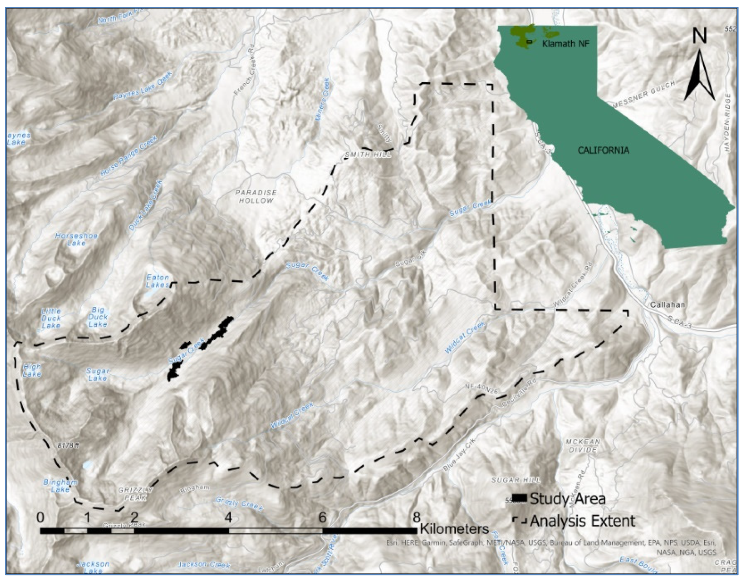
2.1. Study Area
2.2. Biogeography
2.3. Forest Species
2.4. Meteorology and Fire Regime
2.5. Area Solar Radiation, Canopy Structure and Insolation Partitioning
2.6. Data
2.6.1. Multispectral Imagery Data Specification
2.6.2. LiDAR Data Acquisition and Specification
2.7. Methods
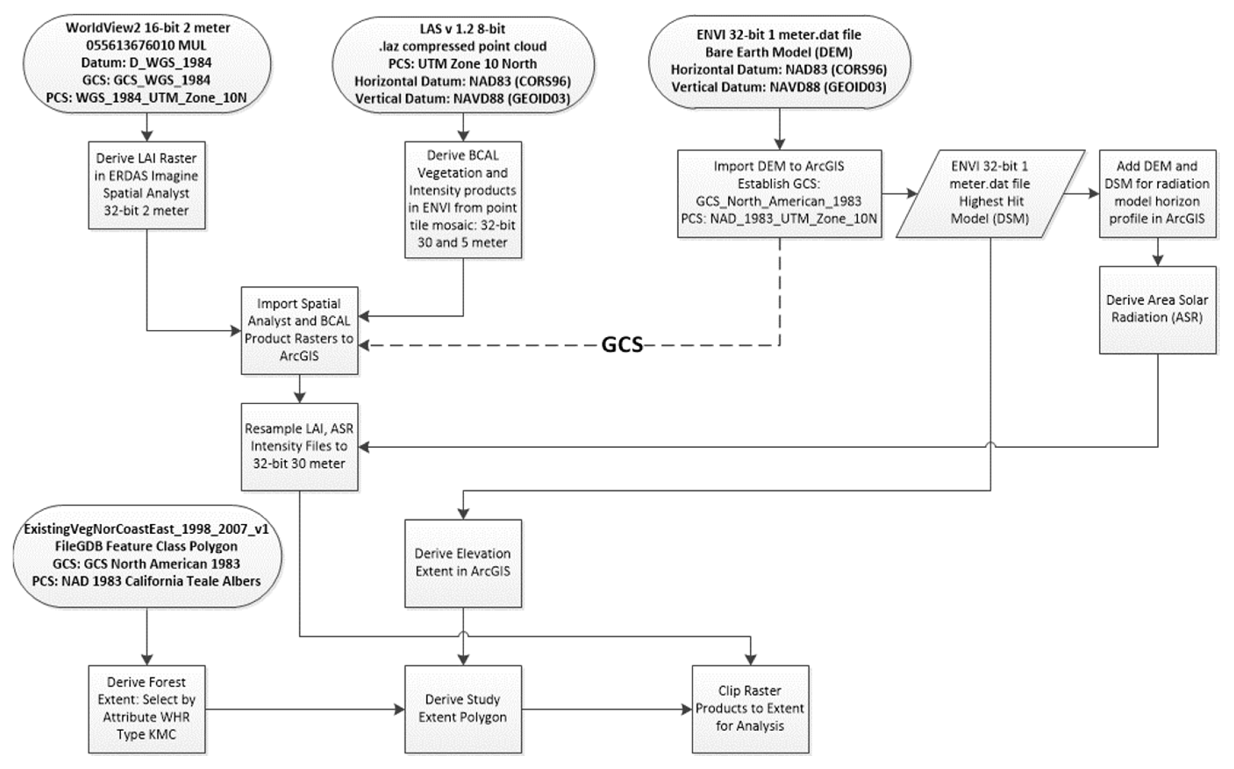
2.7.1. Data Processing Summary
2.7.2. Canopy Structure and Area Solar Radiation Metrics
- t is the proportion of PAR incident at the top of the canopy that is transmitted to a given point x within the canopy;
- LAI(x) is the total leaf area above point x;
- K is the extinction coefficient.
- 1.
- Canopy Height (CHM) in meters was determined from the LiDAR digital surface model (DSM) and the first returns data at 1 m resolution. It was utilized to derive area incident solar radiation adjusted for topography as well as to provide data required for sample plot selection by using the average values at 30 m resolution matched to the gridded canopy metrics raster [40,41,42].
- 2.
- Area Solar Radiation (ASR) in WH/m2 was derived using the sum of 12 monthly values (2015 calendar year) for the analysis extent and resampled to 30 m resolution. ASR was modeled in ArcGIS using the sum of the LiDAR bare earth surface product (DEM) and the canopy height model (CHM) product as the topographic parameter, including topographic elevation data for the entire watershed used as the horizon parameters for the ASR model equations [43,44].Radiation parameters included diffuse model type (radiation flux varied with zenith angle in a non-uniform overcast sky condition), diffuse proportion (proportion of global normal radiation flux that is diffuse by month), and atmospheric transmissivity (fraction of radiation that passes through the atmosphere by month). Input parameters were derived from meteorological data acquired from a field station within close proximity to the analysis extent in 2015.ASR is a term used to describe irradiation, or the sum of downward area irradiance per unit area over a stated time interval expressed in WH/m2. Irradiance is the instantaneous density of solar radiation on a unit area expressed in W/m2. It comprises a global radiation value (Globaltot), or the sum of direct (Dirtot) and diffuse (Diftot) radiation of all sun map and sky map sectors as shown in the solar model equation [43,44]:Dirtot for a given location is the sum of the direct insolation (Dirθ,α) from all sun map sectors. Direct insolation from the sun map sector (Dirθ,α) with a centroid at zenith angle (θ) and azimuth angle (α) is calculated using the following equation:where:
- SConst is the solar flux outside the atmosphere at the mean earth–sun distance, known as solar constant. The solar constant used in the analysis is 1367 W/m2. This is consistent with the World Radiation Center (WRC) solar constant;
- β is the transmissivity of the atmosphere (averaged over all wavelengths) for the shortest path (in the direction of the zenith);
- m(θ) is the relative optical path length, measured as a proportion relative to the zenith path length;
- SunDurθ,α is the time duration represented by the sky sector. For most sectors, it is equal to the day interval (for example, a month) multiplied by the hour interval (for example, a half hour). For partial sectors (near the horizon), the duration is calculated using spherical geometry;
- SunGapθ,α is the gap fraction for the sun map sector;
Total diffuse solar radiation for the location (Diftot) is calculated as the sum of the diffuse solar radiation (Dif) from all the sky map sectors. The diffuse radiation at its centroid (Dif) is calculated, integrated over the input time interval, and corrected by the gap fraction and angle of incidence using the following equation:where:- Rglb is the global normal radiation;
- Pdif is the proportion of global normal radiation flux that is diffused;
- Dur is the time interval for analysis;
- SkyGapθ,α is the gap fraction (proportion of visible sky) for the sky sector;
- Weightθ,α is the proportion of diffuse radiation originating in a given sky sector relative to all sectors;
- 3.
- Intensity of return (IR) is a measure of amplitude describing the peak power ratio of the laser return to the emitted laser, calculated as a function of surface reflectivity. Values are corrected for variability between flight lines and pre-processed at a 0.5 m pixel resolution before being processed using the BCAL vegetation intensity tools and output to a 30 m resolution for the vegetation excluding bare earth data [40,41,42].Research indicates that the returns of high-intensity and the low intensity peak count of the intensity distribution were predictive of live and dead tree biomass, respectively [45].
- 4.
- 5.
- Canopy Relief Ratio is a derived mean height less the minimum height divided by the maximum height less the minimum height per m2 or:This ratio represents the relative shape of the canopy from altimetry observation which describes the degree to which canopy surfaces are in the upper (CRR > 0.5) or in the lower (CRR < 0.5) portions of the height range [41,42,46,47]
- 6.
- 7.
2.7.3. Measures of Biodiversity
- s is the number of different species in your sample;
- N is the total number of individual organisms in the sample.
2.7.4. Multiple Regression Modeling and Cluster Analysis Methods
- Yi is the response variable;
- x1,i, …, xp,i are predictor variables (fixed, nonrandom);
- b0, …, bp are unknown regression coefficients (fixed);
- represents the random error.
- zi is the deviation of an attribute for feature i from its mean;
- wi,j is the spatial weight between feature i and j;
- n is the number of features in the dataset;
- is the aggregate of spatial weights .
- xi and xj are attribute values for features i and j;
- wi,j is the spatial weight between feature i and j;
- n is the number of features in the dataset;
- Indicates that features i and j cannot be the same feature.
2.7.5. Sample Plot Selection
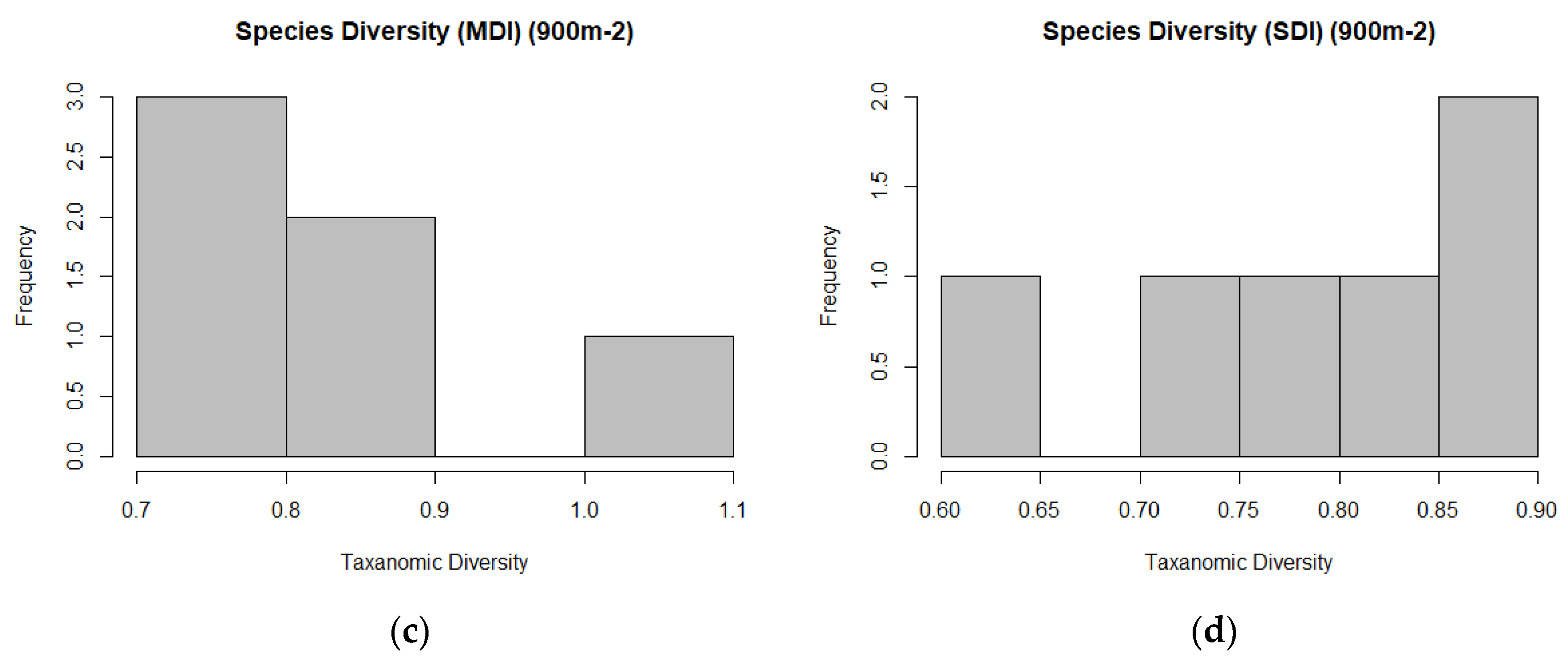
2.7.6. Biodiversity Response Variables
3. Results
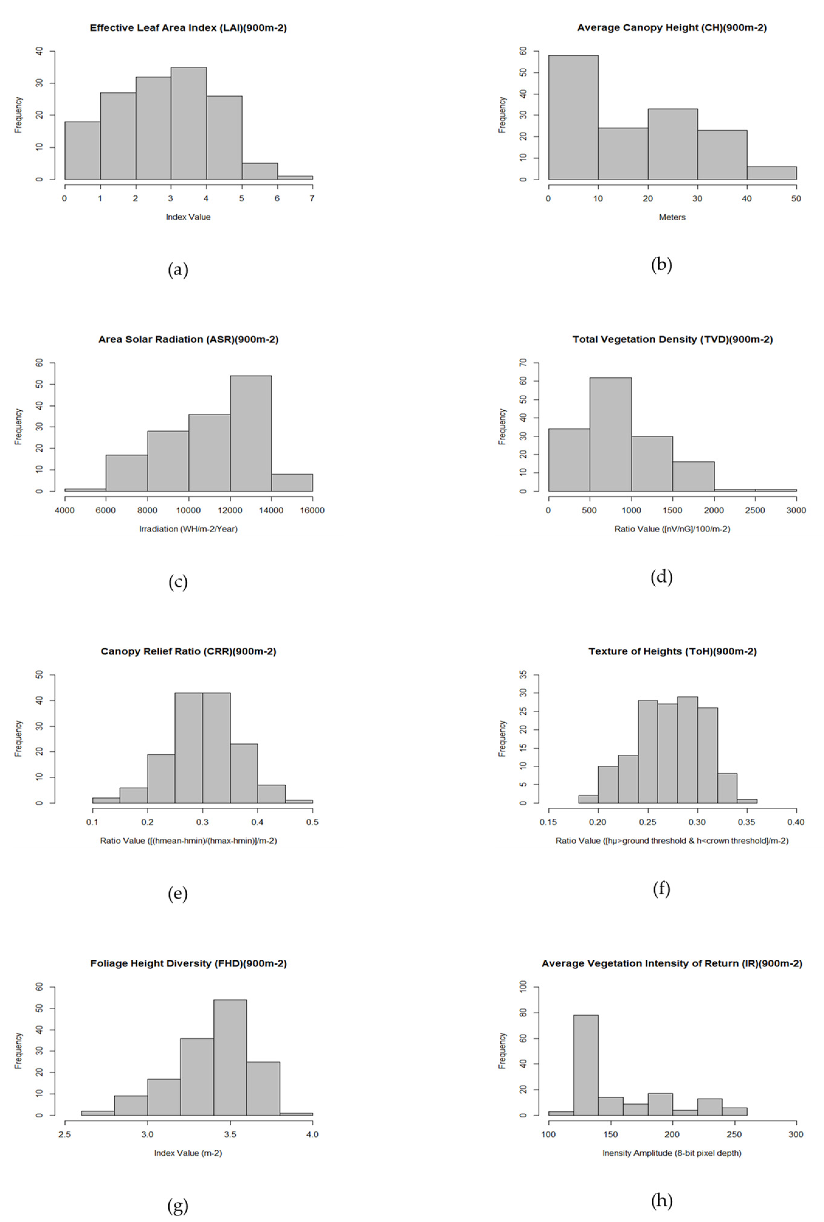
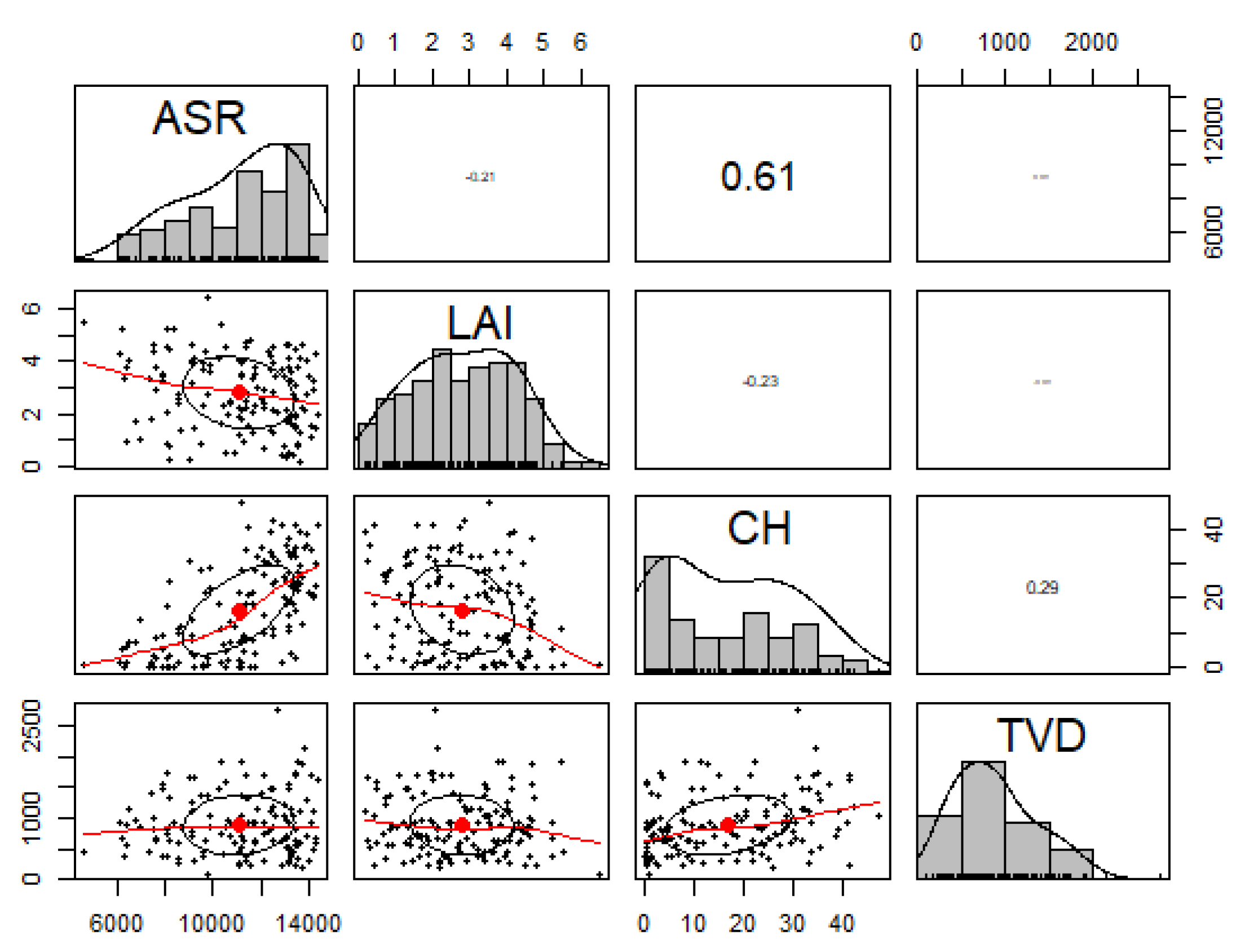
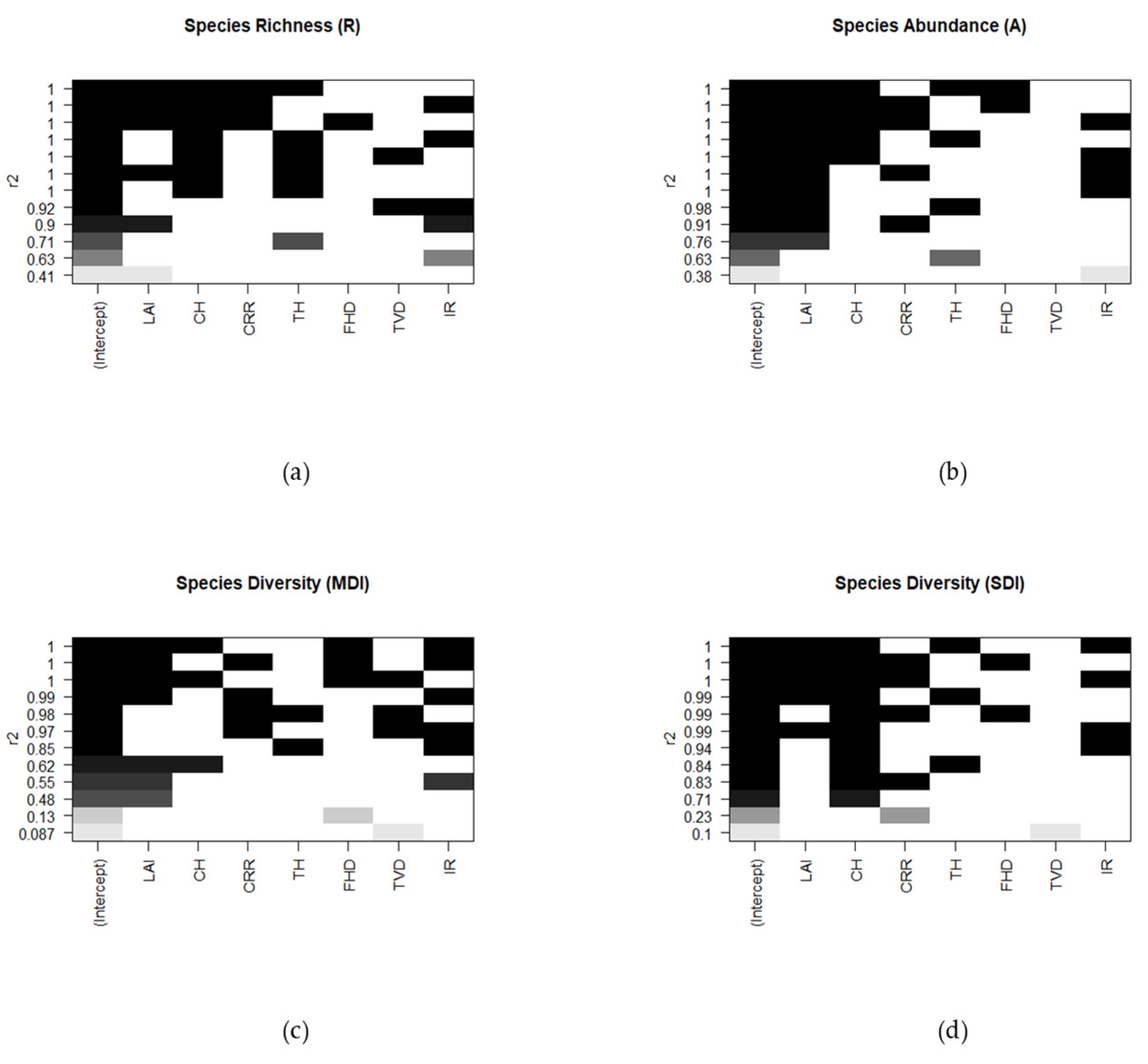
Study Area Predictor Variable Distributions
- p is the specific predictor variable;
- k is the total number of predictor variables.
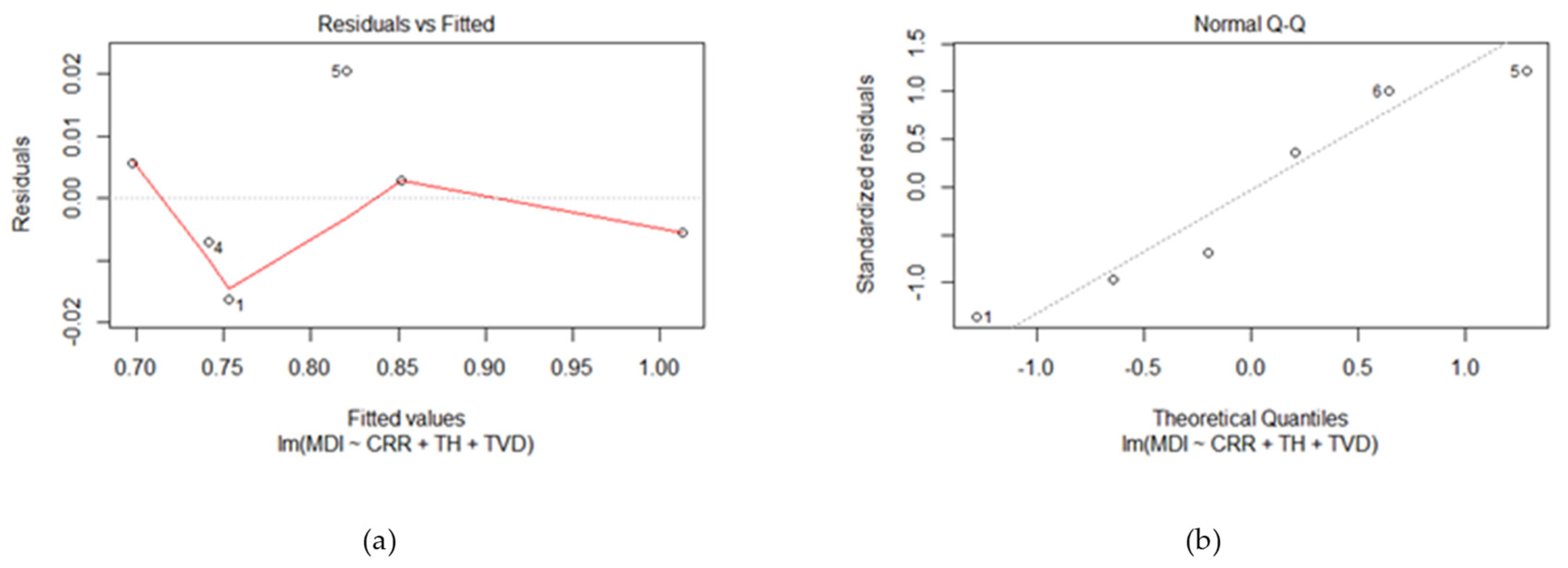
- A linear relationship between the dependent and predictor variables;
- The model errors are independent;
- The model errors are normally distributed;
- The model errors have a constant variance with respect to the predictor variables [53].
- xj is the attribute for feature j;
- wi,j is the spatial weight between features i and j;
- n is the number of features in the dataset and:
4. Conclusions
5. Discussion
Author Contributions
Funding
Acknowledgments
Conflicts of Interest
References
- Levin, S. The problem of pattern and scale in ecology. Ecology 1992, 73, 1943–1967. [Google Scholar] [CrossRef]
- von Humboldt, A.; Bonpland, A. Essai sur la Géographie des Plantes; Levrault, Schoelle et Cie: Paris, France, 1807. [Google Scholar]
- Dufour, A.; Gadallah, F.; Wagner, H.; Guisan, A.; Buttler, A. Plant species richness and environmental heterogeneity in a mountain landscape: Effects of variability and spatial configuration. Ecography 2006, 29, 573–584. [Google Scholar] [CrossRef]
- Schulze, E.-D. Plant Ecology; Springer: Berlin/Heidelberg, Germany, 2005. [Google Scholar]
- Zhang, Y.; Chen, H.; Reich, P. Forest productivity increases with evenness, species richness and trait variation: A global meta-analysis. J. Ecol. 2012, 100, 742–749. [Google Scholar] [CrossRef]
- Ishii, H.; Tanabe, S.; Hiura, T. Exploring the Relationships Among Canopy Structure, Stand Productivity and Biodiversity of Temperate Forest Ecosystems. For. Sci. 2004, 50, 342. [Google Scholar]
- Schneider, F.; Morsdorf, F.; Schmid, B.; Petchey, O.; Hueni, A.; Schimel, D.; Schaepman, M. Mapping functional diversity from remotely sensed morphological and physiological forest traits. Nat. Commun. 2017, 8, 1441. [Google Scholar] [CrossRef] [Green Version]
- Hillenbrand, H. On the generality of the latitudinal diversity gradient. Am. Nat. 2004, 163, 192–211. [Google Scholar] [CrossRef] [Green Version]
- Ali, A. Forest stand structure and functioning: Current knowledge and future challenges. Ecol. Indic. 2019, 98, 665–677. [Google Scholar] [CrossRef]
- Pan, Y.; Birdsey, R.; Phillips, O.; Jackson, R. The Structure, Distribution, and Biomass of the World’s Forests. Annu. Rev. Ecol. Evol. Syst. 2013, 44, 593. [Google Scholar] [CrossRef] [Green Version]
- Ozanne, C.; Anhuf, D.; Boulter, S.; Keller, M.; Kitching, R.; Körner, C.; Melnzer, F.; Mitchell, A.; Nakashizuka, T.; Silva Dias, P.; et al. Biodiversity Meets the Atmosphere: A Global View of Forest Canopies. Science 2003, 301, 183–186. [Google Scholar] [CrossRef] [Green Version]
- Gao, T.; Hedblom, M.; Emilsson, T.; Busse Nielsen, A. The role of forest stand structure as biodiversity indicator. For. Ecol. Manag. 2014, 330, 82–93. [Google Scholar] [CrossRef]
- Schoonmaker, P.; McKee, A. Species Composition and Diversity During Secondary Succession of Coniferous Forests in the Western Cascade Mountains of Oregon. For. Sci. 1988, 34, 960–979. [Google Scholar]
- Donato, D.; Fontaine, J.; Robinson, W.; Kauffman, J.; Law, B. Vegetation response to a short interval between high-severity wildfires in a mixed-evergreen forest. J. Ecol. 2009, 97, 142–154. [Google Scholar] [CrossRef] [Green Version]
- Pan, Y.; Chen, J.M.; Birdsey, R.; McCullough, K.; He, L.; Deng, F. Age structure and disturbance legacy of North American forests. Biogeosciences 2011, 8, 715–732. [Google Scholar] [CrossRef] [Green Version]
- Leiterer, R.; Furrer, R.; Schaepman, M.; Morsdorf, F. Forest canopy-structure characterization: A data-driven approach. For. Ecol. Manag. 2015, 358, 48–61. [Google Scholar] [CrossRef]
- Klamath-Siskiyou. Available online: http://www.worldwildlife.org/ecoregions/na0516 (accessed on 1 December 2016).
- Keeler-Wolf, T. Ecological Surveys of Forest Service Research Natural Areas in California; Gen. Tech. Rep. PSW-125; Pacific Southwest Research Station, Forest Service, U.S. Department of Agriculture: Berkeley, CA, USA, 1990; 177p.
- Küchler, A.W. Appendix: The map of the natural vegetation of California. In Terrestrial Vegetation of California; Barbour, M., Major, J., Eds.; John Wiley and Sons: New York, NY, USA, 1977; pp. 909–938. [Google Scholar]
- Sawyer, J.; Thornburgh, D.; Griffin, J. Mixed evergreen forest. In Terrestrial Vegetation of California; Barbour, M., Major, J., Eds.; John Wiley and Sons: New York, NY, USA, 1977; pp. 359–382. [Google Scholar]
- Skinner, C.; Taylor, A.; Agee, J. Klamath Mountains bioregion. In Fire in California’s Ecosystems; Sugihara, N., van Wagtendonk, J., Fites-Kaufman, J., Shaffer, K., Thode, A., Eds.; University of California Press: Berkeley, CA, USA, 2006; pp. 170–194. [Google Scholar]
- DeSiervo, M.; Jules, E.; Kauffmann, M.; Bost, D.; Butz, R. Revisiting John Sawyer and Dale Thornburgh’s 1969 Vegetation Plots in the Russian Wilderness: A Legacy Continued. Fremontia 2016, 44, 20–25. [Google Scholar]
- Olseth, J.; Skartveit, A. Spatial distribution of photosynthetically active radiation over complex topography. Agric. For. Meteorol. 1997, 86, 205–214. [Google Scholar] [CrossRef]
- Oliphant, A.; Susan, C.; Grimmond, B.; Schmid, H.-P.; Wayson, C. Local-scale heterogeneity of photosynthetically active radiation (PAR), absorbed PAR and net radiation as a function of topography, sky conditions and leaf area index. Remote Sens. Environ. 2006, 103, 324–337. [Google Scholar] [CrossRef]
- Nunez, M. The calculation of solar and net radiation in mountainous terrain. J. Biogeogr. 1980, 7, 173–186. [Google Scholar] [CrossRef]
- Smith, M.-L.; Anderson, J.; Fladeland, M. Forest Canopy Structural Properties. In Field Measurements for Forest Carbon Monitoring; Hoover, C.M., Ed.; Springer Science+Business Media B.V.: New York, NY, USA, 2008; pp. 179–196. [Google Scholar]
- Geiger, R. The Climate near the Ground; Harvard University Press: Cambridge, MA, USA, 1965. [Google Scholar]
- Hamilton, R.; Cushman, S.; McCallum, K.; McCusker, N.; Mellin, T.; Nigrelli, M.; Williamson, M. Multiscale Landscape Pattern Monitoring Using Remote Sensing: The Four-Forest Restoration Initiative; RSAC-10022-RPT1; U.S. Department of Agriculture, Forest Service, Remote Sensing Applications Center: Salt Lake City, UT, USA, 2013; 24p.
- Pacific Southwest Region. Existing Vegetation-CALVEG; ESRI geodatabase; USDA-Forest Service, Pacific Southwest Region: McClellan, CA, USA, 2017.
- DigitalGlobe. WorldView2 Image 055613676010; DigitalGlobe: Longmont, CO, USA, 2013. [Google Scholar]
- Chen, J.; Black, T. Defining leaf area index for non-flat leaves. Agric. For. Meteorol. 1992, 57, 1–12. [Google Scholar] [CrossRef]
- Asner, G.; Scurlock, J.; Hicke, J. Global synthesis of leaf area index observations: Implications for ecological and remote sensing studies. Glob. Ecol. Biogeogr. 2003, 12, 191–205. [Google Scholar] [CrossRef] [Green Version]
- Perry, D.; Oren, R.; Hart, S. Forest Ecosystems; Johns Hopkins University Press: Baltimore, MD, USA, 2008. [Google Scholar]
- Wulder, M.; LeDrew, E.; Franklin, S.; Lavigne, M. Aerial image texture information in the estimation of northern deciduous and mixed wood forest leaf area index (LAI). Remote Sens. Environ. 1998, 64, 64–76. [Google Scholar] [CrossRef]
- Normalized Difference Vegetation Index (NDVI) Analysis for Forestry and Crop Management. Available online: http://simwright.com/downloads/SimWright_NDVI.pdfSlide2. (accessed on 1 May 2019).
- Attenuation Coefficient. Available online: https://en.wikipedia.org/w/index.php?title=Attenuation_coefficientandoldid=925582822 (accessed on 1 December 2019).
- Saitoh, T.; Shin, N.; Noda, H.; Muraoka, H.; Nasahara, K. Examination of the extinction coefficient in the Beer–Lambert law for an accurate estimation of the forest canopy leaf area index. For. Sci. Technol. 2012, 8, 67–76. [Google Scholar] [CrossRef]
- Zhang, L.; Hu, Z.; Fan, J.; Zhou, D.; Tang, F. A meta-analysis of the canopy light extinction coefficient in terrestrial ecosystems. Front. Earth Sci. 2014, 8, 599–609. [Google Scholar] [CrossRef]
- “Leaf Area Index—Fraction of Photosynthetically Active Radiation 8-Day L4 Global 1km.” MOD15A2 | LP DAAC NASA Land Data Products and Services. Available online: https://lpdaac.usgs.gov/dataset_discovery/modis/modis_products_table/mod15a2 (accessed on 2 December 2017).
- QSI Environmental. Technical Data Report-USFS PSW Region 5 LiDAR; USDA-Forest Service, Pacific Southwest Region: McClellan, CA, USA, 2015.
- Boise Center Aerospace Laboratory Lidar Tools. Available online: http://bcal.boisestate.edu/tools/lidar (accessed on 30 April 2017).
- Fu, P.; Rich, P. The Solar Analyst 1.0 Manual; Helios Environmental Modeling Institute: Lawrence, KS, USA, 2000.
- Fu, P.; Rich, P. A Geometric Solar Radiation Model with Applications in Agriculture and Forestry. Comput. Electron. Agric. 2002, 37, 25–35. [Google Scholar] [CrossRef]
- Evans, J.; Hudak, A.; Faux, R.; Smith, A. Discrete Return Lidar in Natural Resources: Recommendations for Project Planning, Data Processing, and Deliverables. Remote Sens. 2009, 1, 776–794. [Google Scholar] [CrossRef] [Green Version]
- Kim, Y.; Yang, Z.; Cohen, W.; Pflugmacher, D.; Lauver, C.; Vankat, J. Distinguishing between Live and Dead Standing Tree Biomass on the North Rim of Grand Canyon National Park, USA Using Small-Footprint Lidar Data. Remote Sens. Environ. 2009, 113, 2499–2510. [Google Scholar] [CrossRef]
- Pike, R.; Wilson, S. Elevation-Relief Ratio, Hypsometric Integral and Geomorphic Area-Altitude Analysis. Geol. Soc. Am. Bull. 1971, 82, 1079–1084. [Google Scholar] [CrossRef]
- Parker, G.; Russ, M. The canopy surface and stand development: Assessing forest canopy structure and complexity with near-surface altimetry. For. Ecol. Manag. 2004, 189, 307–315. [Google Scholar] [CrossRef]
- Whittaker, R. Vegetation of the Siskiyou Mountains, Oregon and California. Ecol. Monogr. 1960, 30, 279–338. [Google Scholar] [CrossRef]
- Ricklefs, R.; Miller, G. Ecology, 4th ed.; W.H. Freeman: New York, NY, USA, 2000. [Google Scholar]
- Whittaker, R. Evolution and Measurement of Species Diversity. Taxon 1972, 21, 213–251. [Google Scholar] [CrossRef] [Green Version]
- Faith, D. Conservation evaluation and phylogenetic diversity. Biol. Conserv. 1992, 61, 1–10. [Google Scholar] [CrossRef]
- Guisan, A.; Zimmermann, N. Predictive habitat distribution models in ecology. Ecol. Model. 2000, 135, 147–186. [Google Scholar] [CrossRef]
- USDA. Technical Report-USFS Remote Sensing Applications Center; USDA-Forest Service-RSAC: Salt Lake City, UT, USA, 2016.
- Hao, M.; Zhang, C.; Zhao, X.; von Gadow, K. Functional and phylogenetic diversity determine woody productivity in a temperate forest. Ecol. Evol. 2018, 2018, 1–12. [Google Scholar] [CrossRef] [PubMed]
- Cornelissen, J.; Lavorel, S.; Garnier, E.; Diaz, S.; Buchmann, N.; Gurvich, D.; Reich, P.; ter Steege, H.; Morgan, H.; van der Heijden, M.; et al. A handbook of protocols for standardized and easy measurement of plant functional traits worldwide. Aust. J. Bot. 2003, 51, 335–380. [Google Scholar] [CrossRef] [Green Version]
- Petchey, O.; O’Gorman, E.; Flynn, D. A functional guide to functional diversity measures. In Biodiversity, Ecosystem Functioning and Human Wellbeing: An Ecological and Economic Perspective; Oxford University Press: Oxford, UK, 2009. [Google Scholar]
- Mason, N.; Mouillot, D.; William, L.; Wilson, J. Functional richness, functional evenness and functional divergence: The primary components of functional diversity. Oikos 2005, 111, 112–118. [Google Scholar] [CrossRef]
- Laureto, L.; Cianciaruso, M.; Samia, D. Functional diversity: An overview of its history and applicability. Nat. Conserv. 2015, 13, 112–116. [Google Scholar] [CrossRef] [Green Version]


| Location | Incoming Solar Radiation (Absorption) | Outgoing Shortwave Radiation (Reflectance) |
|---|---|---|
| Space | 100% | 31% |
| Atmosphere | Absorbed by water vapor, aerosols and O3: 16% Absorbed by clouds: 4% | Back scattered: 6% Reflected by clouds: 16% |
| Surface | 49% | Reflected by land surface: 9% |
| Plot | Richness (R) | Abundance (A) | MDI | SDI |
|---|---|---|---|---|
| 1 | 14 | 361 | 0.737 | 0.829 |
| 2 | 15 | 222 | 1.007 | 0.629 |
| 3 | 18 | 655 | 0.703 | 0.866 |
| 4 | 18 | 601 | 0.734 | 0.723 |
| 5 | 11 | 171 | 0.841 | 0.852 |
| 6 | 22 | 662 | 0.855 | 0.771 |
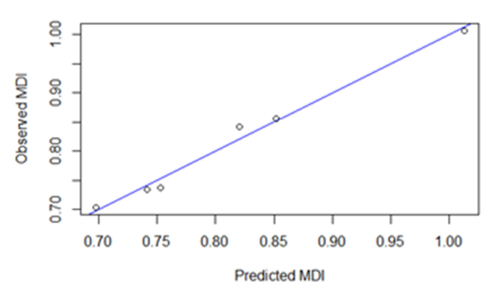
| Model | LAI + CH + IR (Lm0) | LAI + CH (Lm1) | CH + IR + CH:IR (Lm2) | CRR + TH + TVD (Lm3) |
|---|---|---|---|---|
| Adjusted r2 | 0.94 | −0.3252 | 0.693 | 0.9687 |
| F statistic | 22.24 | 0.38 | 4.763 | 52.53 |
| p-value | 0.1544 | 0.709 | 0.1784 | 0.01874 |
| Coefficient significance | CH/0.05 | N/A | CH, IR, CH:IR/0.05 | CRR, TVD/0.001; TH/0.01 |
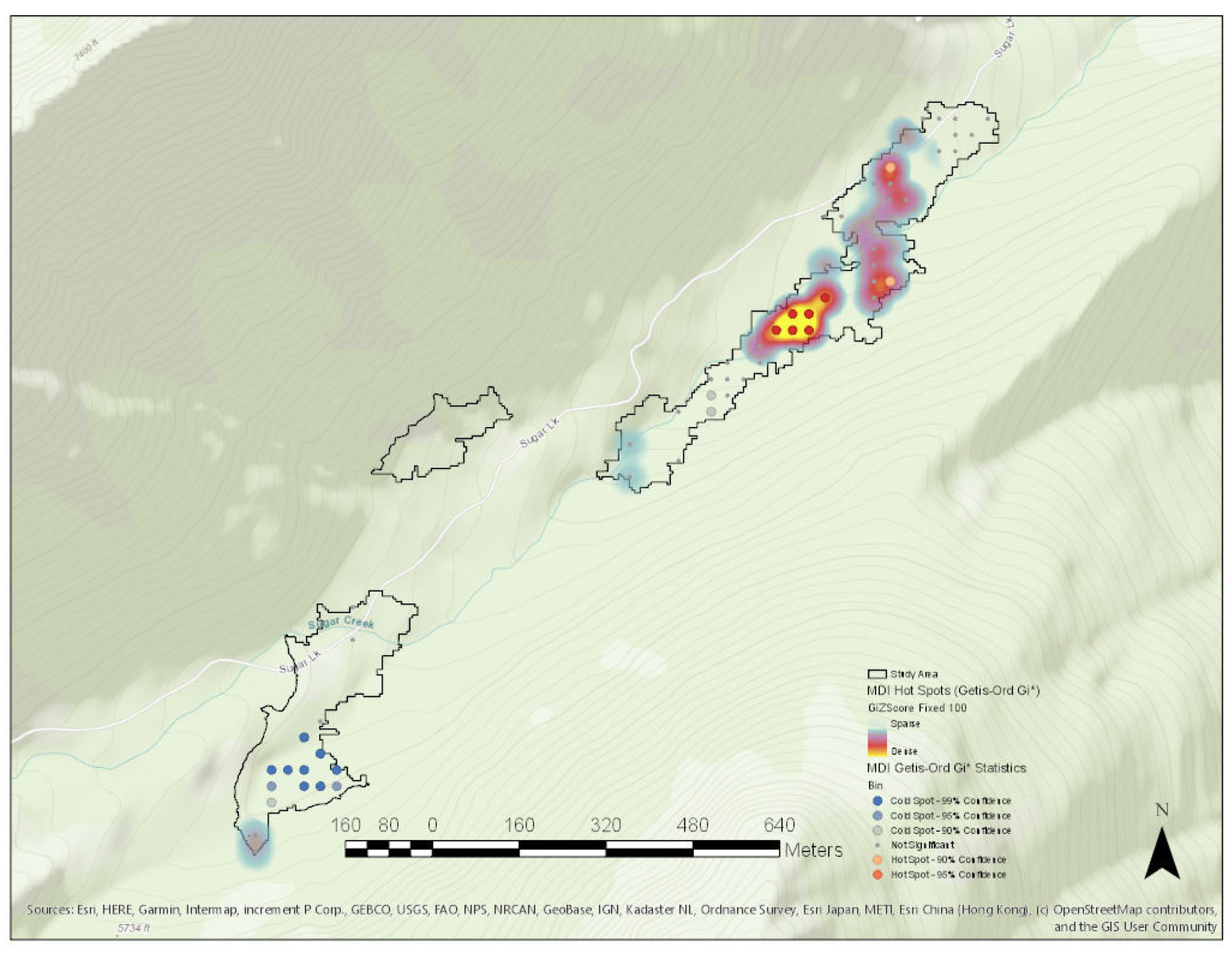
| Global Moran’s I | Getis-Ord General G | ||
|---|---|---|---|
| Moran’s Index | 0.261149 | Observed General G | 0.002234 |
| Expected Index | −0.016667 | Expected General G | 0.002245 |
| Variance | 0.004745 | Variance | 0.000000 |
| z-score | 4.033045 | z-score | −0.162268 |
| p-value | 0.000055 | p-value | 0.871095 |
Publisher’s Note: MDPI stays neutral with regard to jurisdictional claims in published maps and institutional affiliations. |
© 2021 by the authors. Licensee MDPI, Basel, Switzerland. This article is an open access article distributed under the terms and conditions of the Creative Commons Attribution (CC BY) license (https://creativecommons.org/licenses/by/4.0/).
Share and Cite
Dunn, P.C.; Blesius, L. Modeling Insolation, Multi-Spectral Imagery and LiDAR Point-Cloud Metrics to Predict Plant Diversity in a Temperate Montane Forest. Geographies 2021, 1, 79-103. https://doi.org/10.3390/geographies1020006
Dunn PC, Blesius L. Modeling Insolation, Multi-Spectral Imagery and LiDAR Point-Cloud Metrics to Predict Plant Diversity in a Temperate Montane Forest. Geographies. 2021; 1(2):79-103. https://doi.org/10.3390/geographies1020006
Chicago/Turabian StyleDunn, Paul Christian, and Leonhard Blesius. 2021. "Modeling Insolation, Multi-Spectral Imagery and LiDAR Point-Cloud Metrics to Predict Plant Diversity in a Temperate Montane Forest" Geographies 1, no. 2: 79-103. https://doi.org/10.3390/geographies1020006
APA StyleDunn, P. C., & Blesius, L. (2021). Modeling Insolation, Multi-Spectral Imagery and LiDAR Point-Cloud Metrics to Predict Plant Diversity in a Temperate Montane Forest. Geographies, 1(2), 79-103. https://doi.org/10.3390/geographies1020006