Abstract
Measurements of atmospheric pressure by mesoscale transects of vehicle platforms such as the National Severe Storms Lab (NSSL) mobile mesonets have previously been collected in various targeted field campaigns. The challenges involved were specifically documented in the very different environments of tornadogenesis (Markowski et al., 2002) and orographic foehn winds (Raab and Mayr 2008). In recent years, the Jackson State University Mobile Meteorology Unit (MMU) has been developed with broad ranging applications in mind. Barometric pressure was originally expected only to be used for calculation of potential temperature over transects with significant elevation change. Previous studies have determined a dynamic change in measured pressure due to vehicle motion relative to the air that varies quadratically with speed, in agreement with theoretical expectations. This quadratic relationship is examined for the MMU under a variety of conditions. In order to consider least squares regression of this relationship, it was necessary to also have accurate speed and elevation data. Since even quite small elevation changes can produce measurable pressure changes, it was considered necessary to reduce pressures in each transect to the mean elevation using the methodology of Markowski et al. (2002). This required a combination of digital elevation model (DEM) and geographic positioning system (GPS) data to have sufficiently accurate elevations matched to the locations of the pressure measurements. Speed relative to ground from the GPS was used in place of actual air flow speed. Cases to be discussed include transects from approximately 20 to 200 km in length: approximately uniform conditions in flat terrain; crossing of orographic barriers; and cold fronts. Differences between pressure data collected with and without a pressure port are also considered. The impacts for determination of mesoscale pressure gradients, potential temperature, and other derived quantities will be evaluated.
1. Introduction
The first documentation of collecting atmospheric surface pressure from mobile vehicle platforms was reported by Straka et al. in 1996 [1]. The original application was the mobile mesonet component of the Verification of the Origins of Rotation in Tornadoes Experiment (VORTEX), which was operated by the National Severe Storms Laboratory (NSSL). Pressure data from the NSSL mobile mesonet have been used in studies of surface vortex development in severe convective storms during VORTEX and other field campaigns [2]. A parallel application to mesoscale forcing during severe orographic windstorms was reported from field campaigns in the Alps and Sierra Nevada [3,4].
The dynamic pressure effect of air flow past a vehicle is predicted by Bernoulli’s Law to decrease the measured pressure in proportion to the square of the relative air speed:
where is the pressure observed while in motion, is the stationary pressure, is density, and is the relative air flow speed. While the exact form does not strictly apply due to complex flow distortions by the vehicle and location of the barometric sensor, previous studies [1,3] have reported a quadratic relationship to vehicle speed. If it is assumed that, typically, the relative air flow due to the vehicle motion is significantly faster than the ambient wind flow, then the relationship between and can be expected to be affected by:
- Vehicle aerodynamics (shape);
- Location of the barometer on the vehicle;
- Air density.
Broadly speaking, the options for position of the barometer are: above the vehicle on a boom; inside the vehicle; or inside the vehicle but connected to an external pressure port intake. While previous authors have not specifically addressed the effect of air density, it is explicitly included in Bernoulli’s Law and so could be expected to be relevant if it changes sufficiently. The most likely scenario to obtain large air density changes would be due to elevation changes, though potentially, some effect might be noticed across large virtual temperature discontinuities.
It should also be considered what the purposes are for trying to measure pressure on a mobile platform and what environmental conditions are anticipated. Normally mobile platforms are utilized to help elucidate spatial patterns of parameters in greater detail than possible with only stationary sensors, often with assumptions of temporal stationarity, such as the Taylor hypothesis [5]. A distinction should be made, however, between using mobile pressure data to describe horizontal pressure variations (which may be small) [2] and using the data to calculate other desired quantities such as potential temperature [4].
Because surface pressure from even a stationary network of barometers is strongly influenced by elevation differences, it is customary to use various algorithms to adjust data to the same elevation. At synoptic scales, the choice is typically adjusted to mean sea level, while mesoscale studies more often adjust to a local mean elevation. Specifically, how this “reduction” is done may vary according to intended uses, availability of related data (e.g., vertical temperature profile) [3], and reasonableness of the hydrostatic assumption [2].
2. Materials and Methods
2.1. Brief Description of MMU
The development of the Mobile Meteorology Unit (MMU) at Jackson State University (JSU) has proceeded over the last several years primarily to investigate thermodynamic environments and phenomena other than severe storms and foehn winds, ranging from microscales up to smaller synoptic scales. With these purposes in mind, no attempt has been made to measure winds, and pressure was only considered of secondary importance for use in calculating other parameters. A Vaisala PTB101B was first added in 2016 inside the cabin of the vehicle. This was connected to an external Gill pressure port (R.M. Young) above the roof beginning in 2019. Data are typically measured at 2 s intervals and logged on a CR23X datalogger. Position and time are determined from a Garmin GPS16-HVS receiver.
2.2. Data Preparation
The vehicle ground speed (in lieu of measuring relative air flow) is required to calibrate pressures for the Bernoulli effect. The speed is calculated over each measurement interval from the change in GPS position, using spherical earth geometry. Although lateral position accuracy is typically 10 m or less, there are some cases in which forward motion has exhibited high-frequency oscillations that are believed to be from electrical interference. In such cases, a running mean has been applied to the speed without compromising actual speed variations.
Ideally, the actual relationship between and should be determined while moving at constant elevation under homogeneous conditions. In general, this is not practical though, since even a 1 m elevation change corresponds to about 0.1 hPa under standard sea-level conditions. Even to determine the elevation profile of a transect with vertical accuracy of 1 m or better is non-trivial [3]. So, before examining the relationship between and , an estimated profile of elevations along the transect at each measurement time is constructed, and then the measured is adjusted to the mean elevation.
Elevation data are recorded at each measurement time from the GPS with 1 m precision. Unfortunately, the accuracy of elevation from a moving GPS receiver is not consistent, particularly within forests and complex terrain. Various digital elevation model (DEM) datasets exist that have been compiled regionally and globally from satellite, lidar, and ground survey data. When the MMU first began recording barometric data in 2016, it was determined that existing DEM datasets were generally inadequate for use with the mobile data. Two examples that were examined at that time were the Shuttle Radar Topography Mission (SRTM) global data and United States Geological Survey (USGS) 1 min data over the contiguous United States. As of 2021, the USGS “3DEP” program makes available 1/3 arc-second DEM data (nominal 10 m resolution) across the contiguous United States in floating point format with precision down to 0.00001 m vertical, much of which is now based largely on lidar data. In contrast, the DEM data used by Markowski et al. in 2002 [2] were at 30 m resolution and precision of 1 m. Their application was alleviated somewhat by gentle terrain in a rural area with few bridges. With horizontal resolution similar to that of the GPS data and precision less than 1 m, the current USGS data are now adequate over most of the United States for use in processing of mobile pressure data with two caveats:
- The DEM data represent ground level elevations which may be significantly lower than elevated roadways (bridges, overpasses, etc.). In rare cases, the DEM elevations could be also higher than the road elevation passing through a tunnel.
- Approximately a 2 m offset should be applied between the ground surface and the elevation of the barometer on the MMU.
The vehicle offset from ground is easily accommodated. However, the determination of the elevation along elevated roadways requires other data sources. The method employed here is to first create elevation profiles for mobile transects from 10 m DEM data using a geographic information system (GIS) and then to manually examine the data to identify elevated roadway sections using a combination of GPS elevations, pressure data, and aerial photos. Elevations on most bridge sections can be approximated as flat or linearly interpolated between the endpoints. Less commonly, bridges over navigation channels and “flyover” segments of controlled access highways may rise over 30 m above the surface at mid-point. These elevated profiles are estimated based on concurrency of GPS and pressure data. In a few other cases, short segments along causeways had small horizontal GPS errors that were sufficient to put the location in surrounding wetlands that were a few meters lower. These were corrected to keep the elevation close to constant as appropriate.
2.3. Methodology for Cases
Once speed and elevation z are determined as described above, the elevation is slightly smoothed by a 5-point running mean. Using the MMU temperature and humidity data, mean virtual temperature is calculated over the transect and used together with mean elevation in the pressure reduction equation based on Markowski et al. [2]:
where is the gas constant and g is gravitational acceleration. This reduced pressure is then plotted against to obtain a least-squares regression to a quadratic function, which corresponds to Equation (1). With the coefficients of the quadratic function, we can then calculate speed-corrected values of along the transect. If pressure is to be used in calculations of potential temperature and other variables, then it should first be adjusted back from the mean elevation to a “station pressure” at the spatially varying elevation z by inverse application of Equation (2). For the current analyses, no data have been temporally adjusted for secular trends occurring during the transect period.
3. Results and Discussion
3.1. Flat Coastal Terrain with Weak Pressure Gradient (5 April 2021) (Pressure Port)
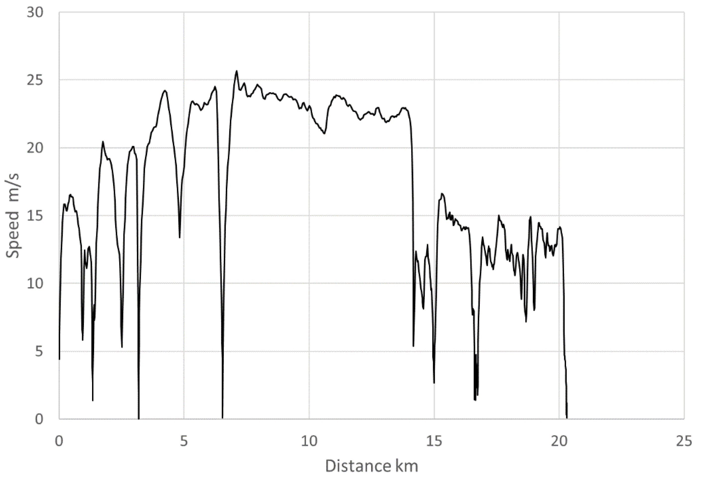
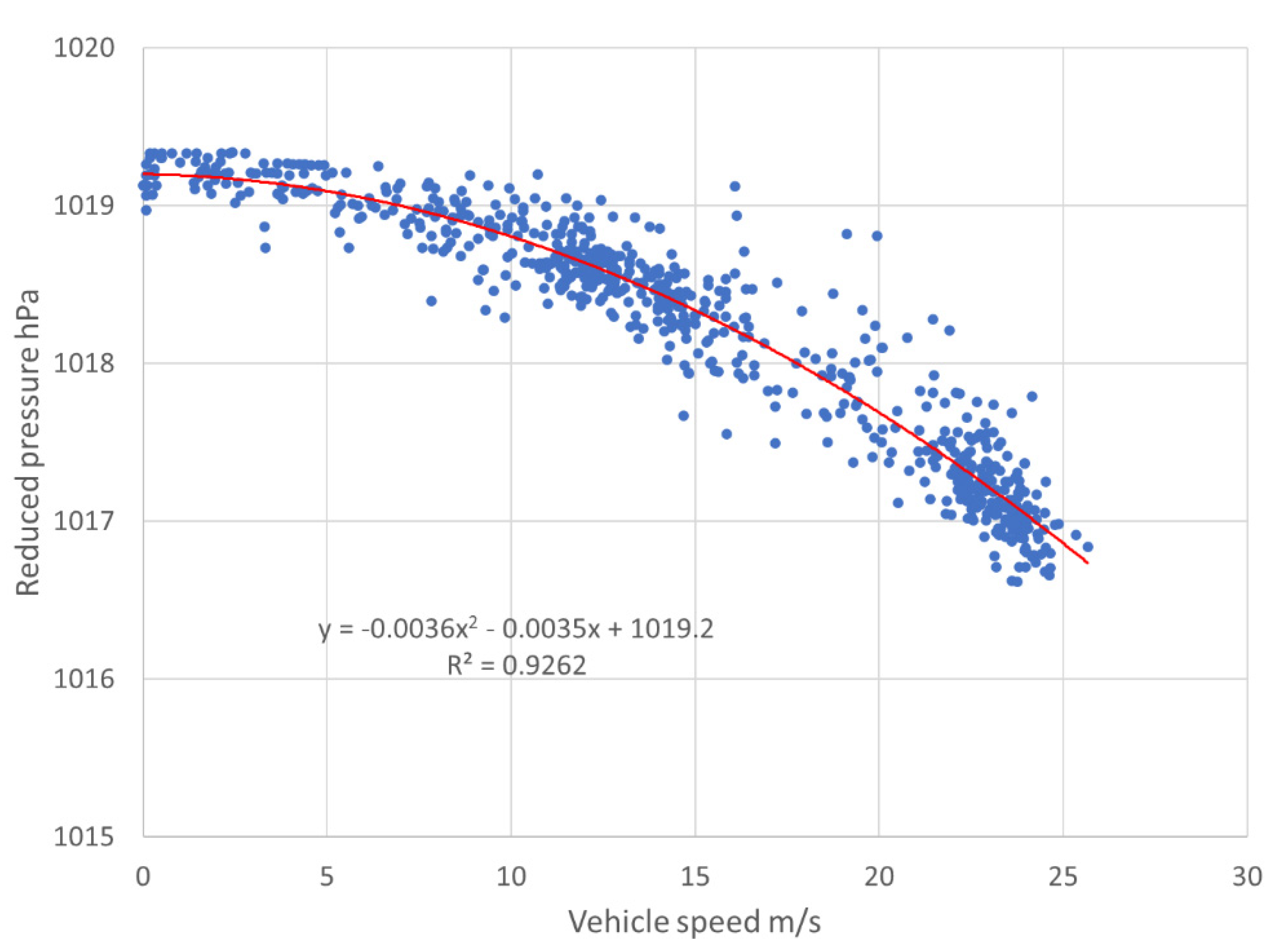
Between 2245–2308 UTC, the MMU drove a 20.3 km transect with minimal elevation change (<5 m) and light winds between Pascagoula, Mississippi, and Bayou Heron (in Grand Bay National Wildlife Refuge) along the coast of the Gulf of Mexico. The vehicle speed ranged from 0 to 25.7 m/s, as shown in Figure 1. Regressing the reduced pressure as a quadratic function of yields the expected decrease with speed from the Bernoulli effect, with an of 0.926 (Figure 2a). In this case, the regression equation is solved for
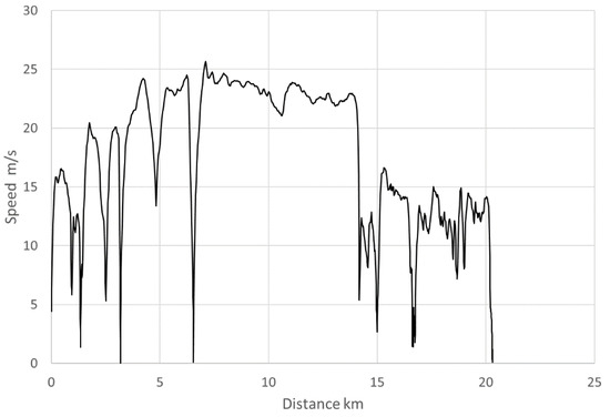
Figure 1.
Vehicle speed from Pascagoula to Bayou Heron.
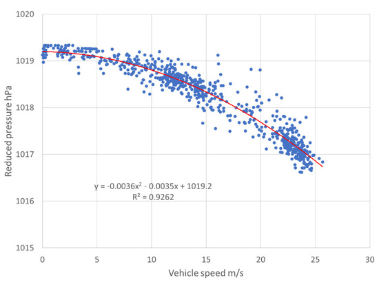
Figure 2.
Quadratic least squares regression of reduced pressure against .
To compensate for the uneven distribution of speeds included in the dataset, the regression is recalculated with binned values of in 2.5 m/s increments of . In this case, the change in is negligible but is increased to 0.997.
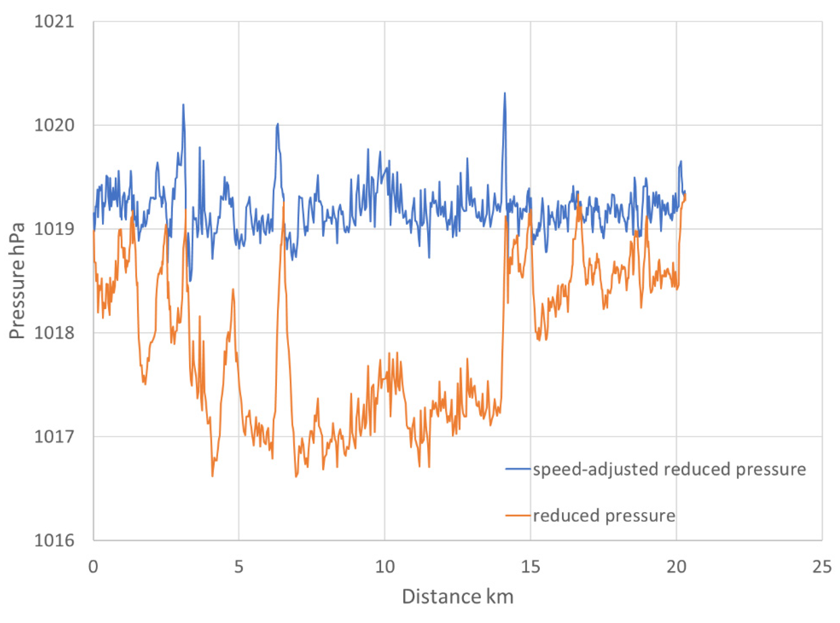
Comparing the reduced pressure with and without speed correction shows differences as large as 2 hPa (Figure 3). Although high-frequency oscillations remain that may be associated with vehicle-induced turbulence and sudden acceleration, the pattern of a nearly constant 1019.2 hPa pressure is much more readily evident after the speed correction. During the period of the transect, the pressure recorded at the nearest synoptic station KPQL (adjusted to ) was 1019.0 hPa.

Figure 3.
Reduced pressure and speed-corrected reduced pressure .
3.2. Strong Cold Front in East Texas (30 April 2017) (No Pressure Port)
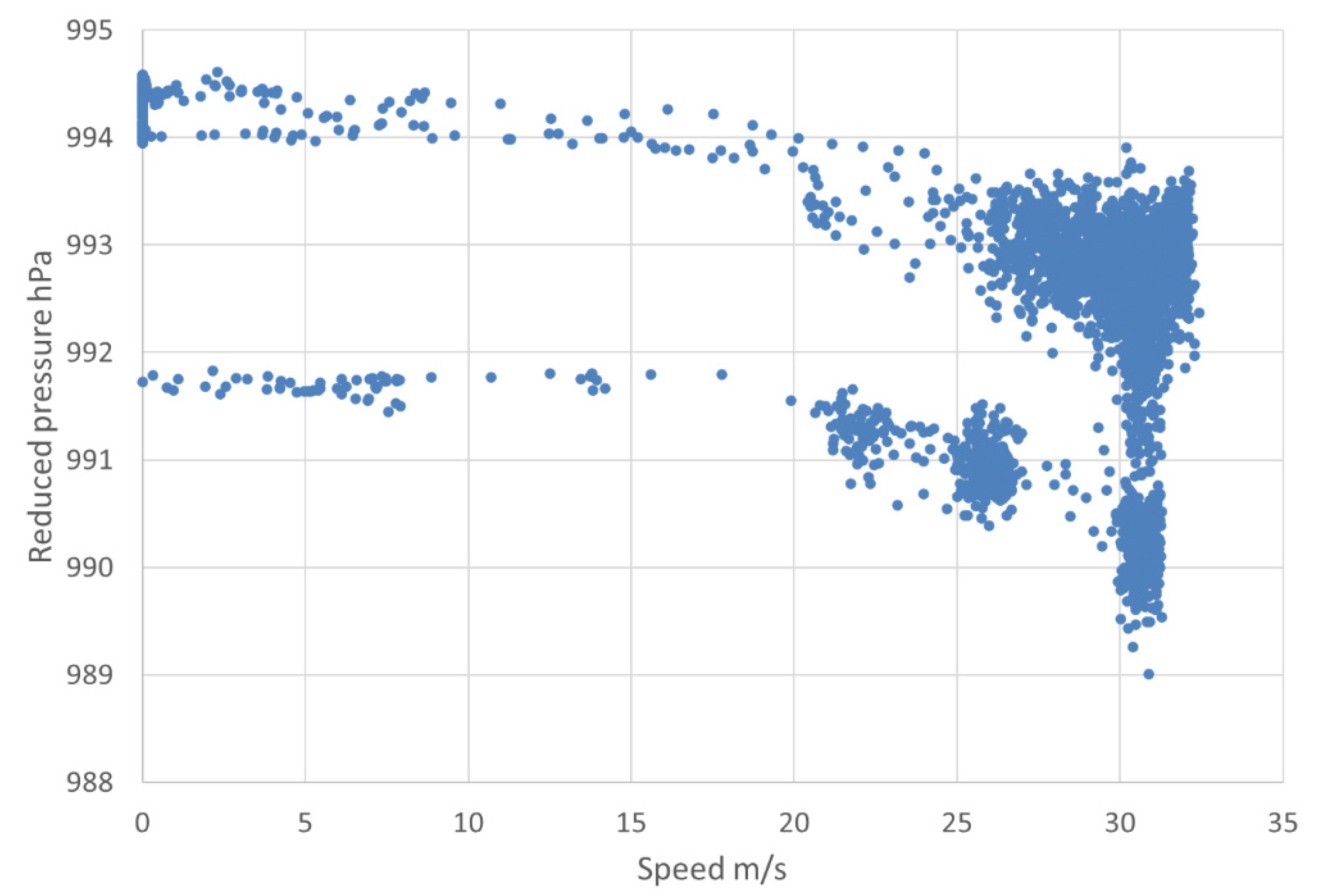
A significantly more dynamically forced case was sampled across a strong cold front that, a few hours before, was associated with violent tornadoes and large hail. The 192 km route extended eastward from a highway rest area in Van Zandt County, Texas to Bossier City, Louisiana between 0412–0613 UTC. Elevations ranged from 52 to 191 m, and temperature rapidly rose by approximately 8 °C as the front was crossed after approximately 150 km. Except for one stop, most of the transect was at highway speeds above 30 m/s. Direct regression along the full transect failed, though evidence of the Bernoulli effect can be seen (Figure 4). Even with binning by speed, regression across the full transect was unsatisfactory (; quadratic coefficient of the wrong sign). However, binned regression separately on each side of the approximate frontal location yielded much better results ( for each). To test the sensitivity of speed adjustment to regression samples, was determined using the regression formula from the first case (Pascagoula) and using regression coefficients from the western subset. Using either approach, the data show a pronounced trough just ahead of the front and rapidly rising pressure in the cooler air (Figure 5). However, the non-local (Pascagoula) regression pressures are approximately 1.5 hPa higher than with local regression. Synoptic station pressures are similar but lacking spatial detail near the front. The mean potential temperature calculated with locally regressed pressure was 291.26 K versus 291.13 K with the non-local regression and 291.37 K with no speed correction applied.

Figure 4.
Reduced pressure versus .
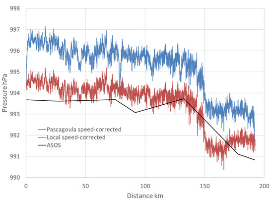
Figure 5.
Speed-corrected reduced pressure using local subset regression and using regression from 5 April 2021 case. Reduced pressures from nearby ASOS synoptic stations plotted for comparison.
3.3. Orographic Barriers
The determination of pressure patterns across significant topography is particularly challenging due to the sparsity of observing stations, uncertainties in reduction to a common elevation, and the tendency of orographic barriers to create relatively complex dynamic patterns [3,6,7]. Two cases will be briefly described that exemplify some of the variety of circumstances.
3.3.1. La Veta Pass in Colorado with Front (18 June 2017) (No Pressure Port)
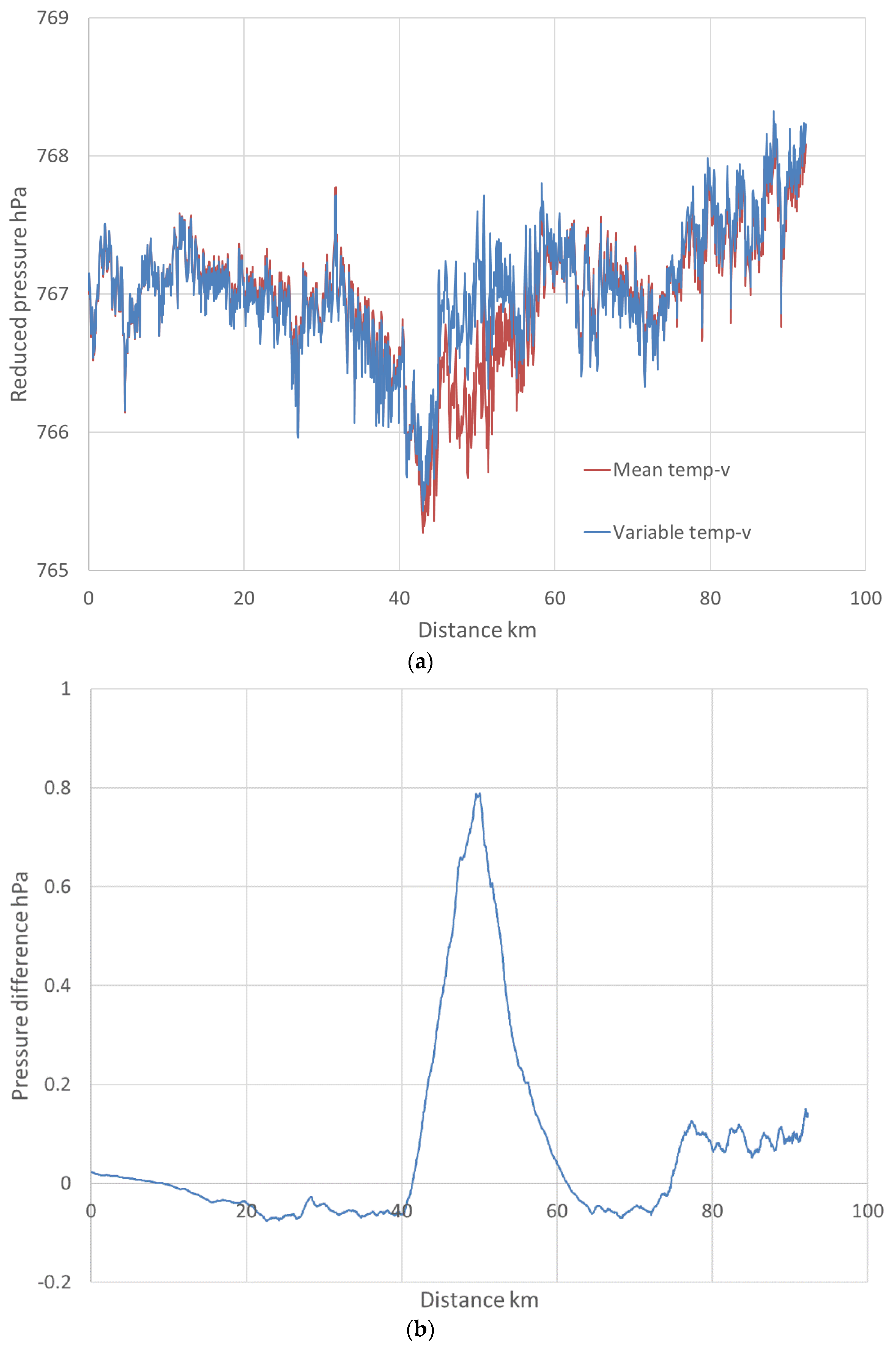
La Veta Pass is a gap in the Sangre de Cristo Mountains southwest of Pueblo, Colorado that connects between the high-elevation San Luis Valley [8] and the western reaches of the Great Plains. The pass was traversed by the MMU from west to east while a back-door cold front was slowly pushing over the mountains from the northeast, in a 92 km transect from east of Alamosa to Walsenburg. The frontal boundary was encountered 10 km west of the crest, so that the western slopes and eastern slopes were in distinctly different air masses. The dichotomy of air masses was not amenable to regression of speed-corrected pressure across the whole transect, though subsets on the west and east slopes separately produced with binning of 0.987 and 0.960. Regardless which set of regression coefficients is used, has a similar pattern with a narrow trough approximately 2 hPa lower near the frontal boundary. Using the (near sea-level) regression from Pascagoula produces reduced pressures nearly 2 hPa higher than local coefficients. Mean reduced pressure values using the western and eastern regressions are 767.0 hPa and 767.4 hPa, respectively.
The front as determined by discontinuity of potential temperature and mixing ratio was at 40 km and the transect highpoint at 50 km. Such an air mass contrast in high terrain provides a stringent test for the use of a constant virtual temperature in Equation 2. Calculation of using locally varying instead of (Figure 6) results in a narrower frontal trough as the cool high-elevation air east of the front indicates pressures as much as 0.8 hPa higher than with the standard pressure reduction based on [2]. This pressure difference makes no significant difference in potential temperature though (<0.001 K), since the same is used in reducing back from to z before calculation of . The speed correction itself changes potential temperature by about 0.1 K.
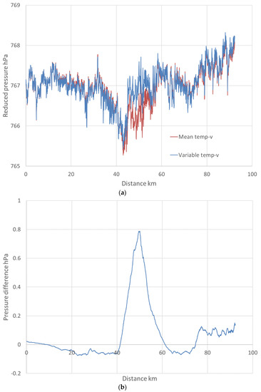
Figure 6.
(a) Speed-corrected reduced pressure from Alamosa County to Walsenburg, with constant or variable virtual temperature. (b) Pressure difference resulting from variation of virtual temperature.
3.3.2. Southern California from San Diego to Plaster City (28–29 July 2017) (No Pressure Port)
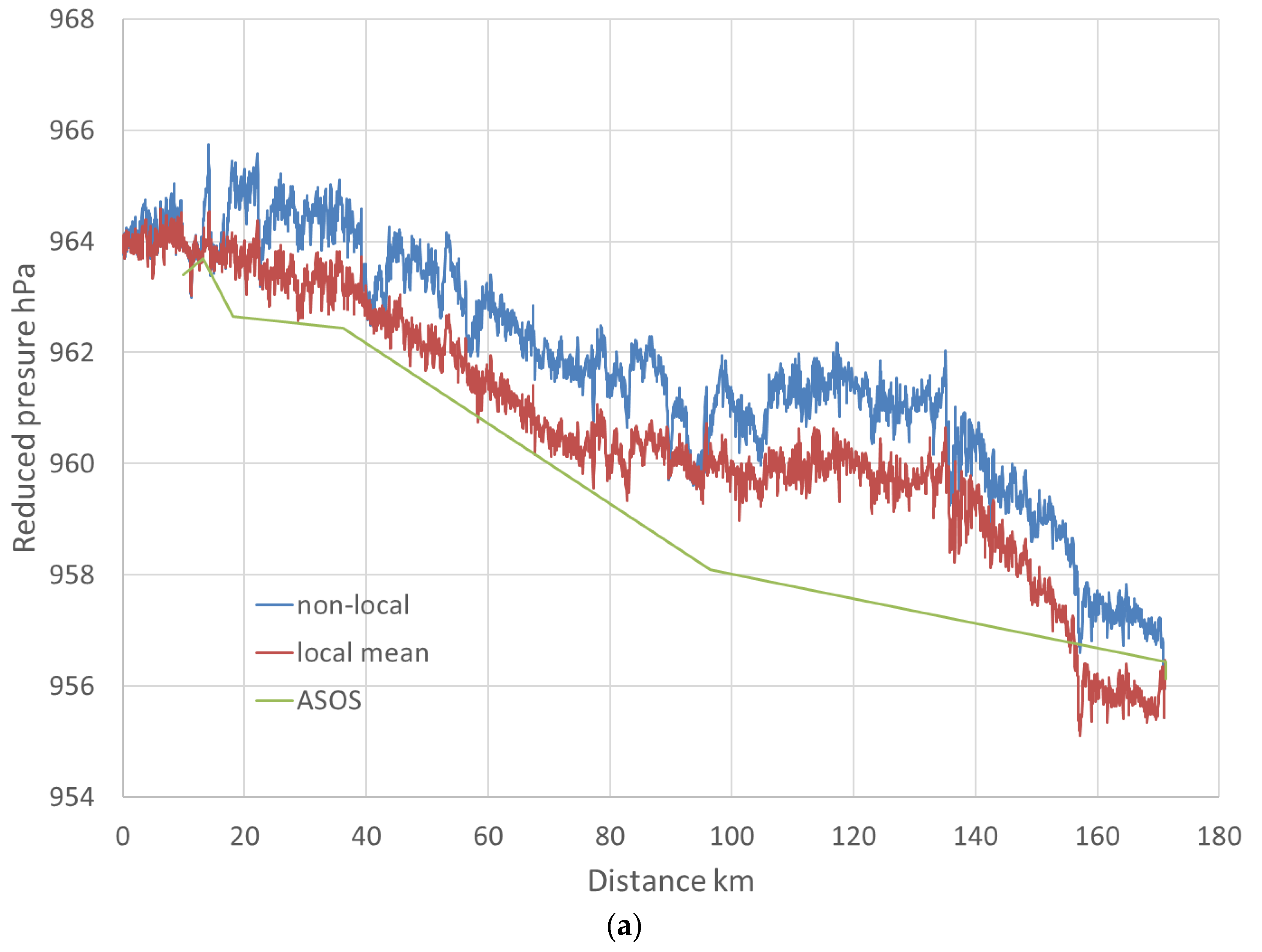
A transect eastward across the Peninsular Ranges of Southern California went from the coastal marine air to the western periphery of the North American monsoon system in the Yuha Desert. The temperature increased dramatically inland from 21 to 41 °C, and winds were light in spite of a pressure drop of approximately 8 hPa over 160 km (Figure 7a). Since there was not a suitable regression across the full distance, the transect was divided into five approximately equal sections to determine regression coefficients. In three of the sections, there was a good relationship with , while the other two were much worse. An average of the coefficients from the three good sections is used as a “local mean”, producing in good agreement was the closest ASOS stations. The need to adjust DEM elevations for bridges and elevated highways is exemplified with this case, with one canyon bridge exceeding 130 m above the terrain. The effect of this elevation discrepancy on the reduced pressure detracts significantly from the real pattern (Figure 7b).
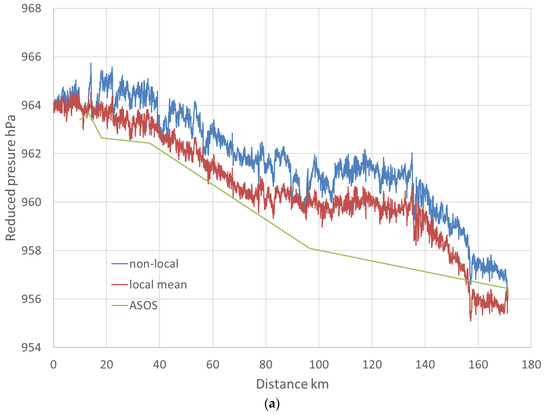
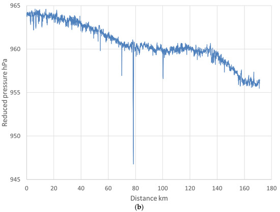
Figure 7.
(a) Speed-corrected reduced pressure from San Diego to Yuha Desert near Plaster City. (b) Speed-corrected reduced pressure using unedited DEM elevations.
3.4. Comparison with and without Pressure Port (23 June 2021)
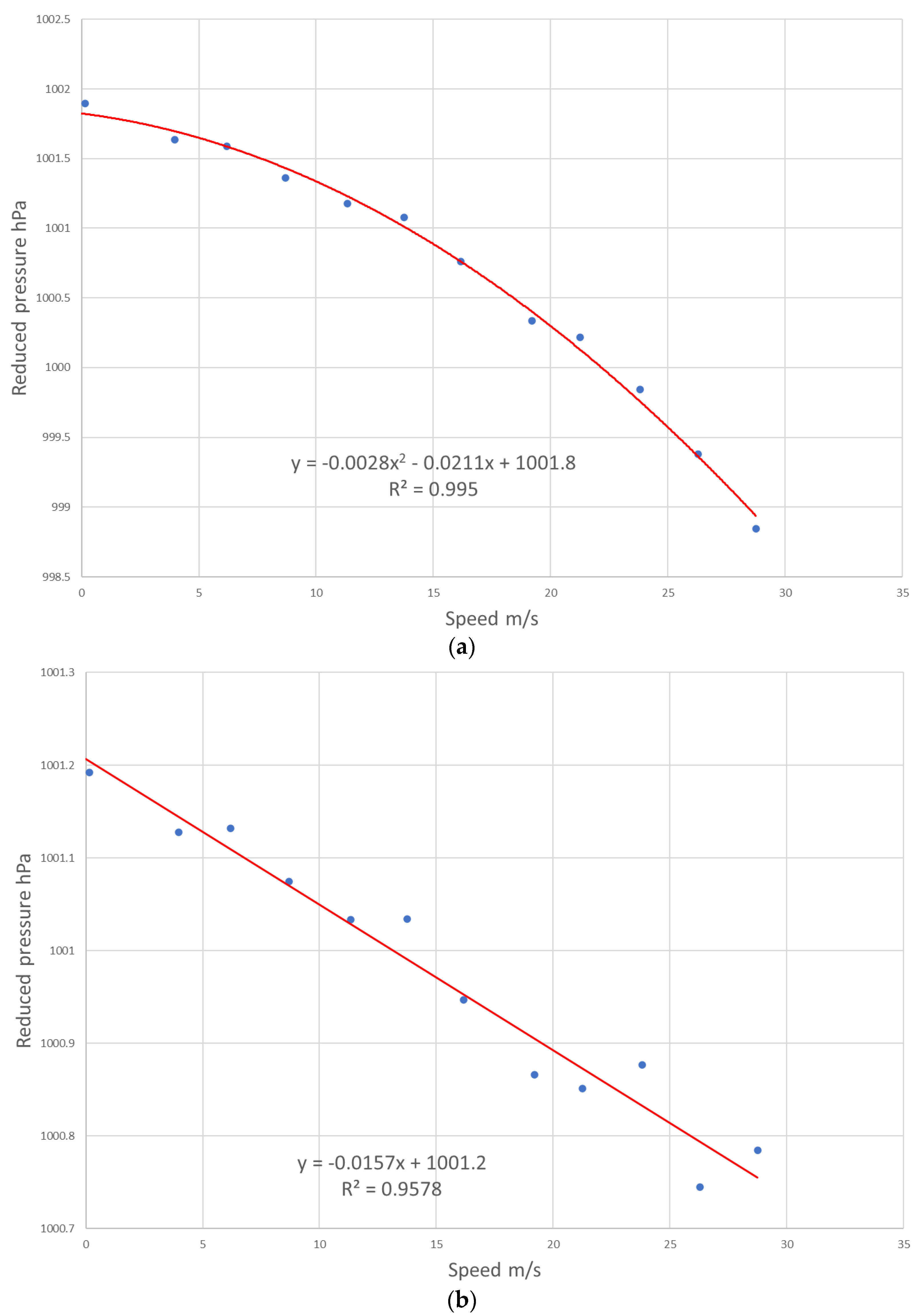
Recently, tests have been done using two barometers concurrently, with and without a pressure port. One example covers a 182 km transect from Jackson to Ackerman, Mississippi, under fair weather conditions. As shown in Figure 8, the binned data from the pressure port varied with speed by about 2.5 hPa and fit very well to a quadratic relationship. However, the data without the port varied by less than 0.5 hPa and fit best to a linear regression with speed.
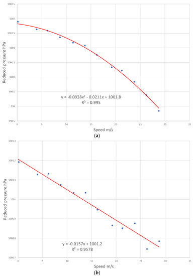
Figure 8.
Least squares regression of reduced pressure against from 23 June 2021 between Jackson and Ackerman, Mississippi: (a) with pressure port (quadratic); (b) without pressure port (linear).
4. Conclusions
- Careful procedures are required to ensure that accurate altitudes are used in “pressure reduction” procedures of mobile barometric data.
- While data over a range of speeds on a perfectly flat road would be ideal for calibration of mobile pressure data, reduction first to a mean altitude as done by Markowski et al. is sufficient to provide data for regression.
- Regression equations are adequate to remove most of the Bernoulli effect from mobile pressure data taken at variable speeds, even under non-ideal conditions of acceleration and vehicle-induced turbulence.
- It seems that data collected using a pressure port exhibit a reduction in pressure with speed that is quadratic, as predicted by Bernoulli. However, data collected within the vehicle cabin without a pressure port show a smaller pressure reduction that is approximately linear.
- Once speed corrections are applied, realistic mesoscale pressure patterns are observable.
- For most applications, the calculation of potential temperature and other derived variables dependent upon pressure is insignificantly influenced by speed effects.
- More cases need to be examined to determine how regression coefficients may vary with air density, in particular at high elevations.
Funding
This research was supported by the NOAA Educational Partnership Program, U.S. Dept. of Commerce (NA11SEC4810003, NA17AE1623) and by the U.S. National Science Foundation (1644888).
Acknowledgments
Mobile data collection during 2017 took place while Loren D. White was on sabbatical appointment at the University of Missouri—Columbia.
Conflicts of Interest
The author declares no conflict of interest. The funders had no role in the design of the study; in the collection, analyses, or interpretation of data; in the writing of the manuscript, or in the decision to publish the results.
References
- Straka, J.M.; Rasmussen, E.N.; Fredrickson, S.E. A mobile mesonet for finescale meteorological observations. J. Atmos. Ocean. Technol. 1996, 13, 921–936. [Google Scholar] [CrossRef] [Green Version]
- Markowski, P.M.; Straka, J.M.; Rasmussen, E.N. Direct surface thermodynamic observations within the rear-flank downdrafts of nontornadic and tornadic supercells. Mon. Weather Rev. 2002, 130, 1692–1721. [Google Scholar] [CrossRef]
- Mayr, G.J.; Vergeiner, J.; Gohm, A. An automobile platform for the measurement of foehn and gap flows. J. Atmos. Ocean. Technol. 2002, 19, 1545–1556. [Google Scholar] [CrossRef]
- Raab, T.; Mayr, G.J. Hydraulic interpretation of the footprints of Sierra Nevada windstorms tracked with an automobile measurement system. J. Appl. Meteorol. Climatol. 2008, 47, 2581–2599. [Google Scholar] [CrossRef]
- Taylor, G.I. The spectrum of turbulence. Proc. Roy. Soc. Lond. Ser. A Math. Phys. Sci. 1938, 164, 476–490. [Google Scholar] [CrossRef] [Green Version]
- Mesinger, F.; Treadon, R.E. “Horizontal” reduction of pressure to sea level: Comparison against the NMC’s Shuell Method. Mon. Weather Rev. 1995, 123, 59–68. [Google Scholar] [CrossRef] [Green Version]
- Pauley, P.M. An example of uncertainty in sea level pressure reduction. Weather Forecast. 1998, 13, 833–850. [Google Scholar] [CrossRef] [Green Version]
- de Boer, G.; Diehl, C.; Jacob, J.; Houston, A.; Smith, Ã.S.; Chilson, P.; Schmale, D.G.; Intrieri, J.; Pinto, J.; Elston, J.; et al. Development of community, capabilities and understanding through unmanned aircraft-based atmospheric research: The LAPSE-RATE campaign. Bull. Am. Meteorol. Soc. 2020, 101, E684–E699. [Google Scholar] [CrossRef] [Green Version]
Publisher’s Note: MDPI stays neutral with regard to jurisdictional claims in published maps and institutional affiliations. |
© 2021 by the author. Licensee MDPI, Basel, Switzerland. This article is an open access article distributed under the terms and conditions of the Creative Commons Attribution (CC BY) license (https://creativecommons.org/licenses/by/4.0/).

