Bias Correction Method Based on Artificial Neural Networks for Quantitative Precipitation Forecast ^†

Abstract

The nowcasting and very short-term prediction system (SisPI, for its acronym in Spanish) is among the tools used by the National Meteorological Service of Cuba for the quantitative precipitation forecast (QPF). SisPI uses the WRF model as the core of its forecasts and one of the challenges to overcome is to improve the precision of the QPF. With this purpose, in this work we present the results of the application of a bias correction method based on artificial neural networks. The method is applied to the highest-resolution domain of SisPI (3 km), and the correction is made from the precipitation estimation of the GPM satellite product. Results shows higher correlation with the artificial neural network model in relation to the values predicted by SisPI (0.76 and 0.34, respectively). The mean square error when applying the artificial neural network model is 3.69, improving the performance of SisPI by 6.78. In general, the bias correction has a good ability to correct the precipitation forecast provided by SisPI, being less evident in cases where precipitation is reported and SisPI is not capable of forecasting it. In cases of overestimation by SisPI (which happens quite frequently), the correction achieves the best results.

1. Introduction

Artificial neural networks are a mathematical technique inspired by biological neural networks [1,2]. At present, the development of this tool continues, being widely used in different branches of science, including atmospheric sciences and related areas [3,4,5]. Within meteorology there are many applications, highlighting its use in the detection of cloud patterns, in weather and climate forecasting, and as a method for correcting forecast errors generated by numerical weather forecast models (NWMs), among others [5].

This research is focused on this last application of ANNs. The work presented is one more contribution that explores the use of artificial neural networks to increase the precision of the numerical forecast, in particular, the quantitative precipitation forecast (QPF). For this purpose, a multi-layer perceptron is used as the network model. It is trained using a configuration obtained in previous studies [5]. As data for the training, the estimation of the satellite precipitation of the GPM product and the precipitation forecast with 3 km of spatial resolution of the nowcasting and very short-term forecast system (SisPI) [6,7,8] are used.

In the section Model and Configuration of the ANN, the information regarding the ANN model and its configuration is presented. The details of the data used, as well as the SisPI description can be found in the section Data Used, while the results achieved for two case studies are discussed in the section Results and Discussion, followed by preliminary conclusions.

2. Model and Configuration of the ANN

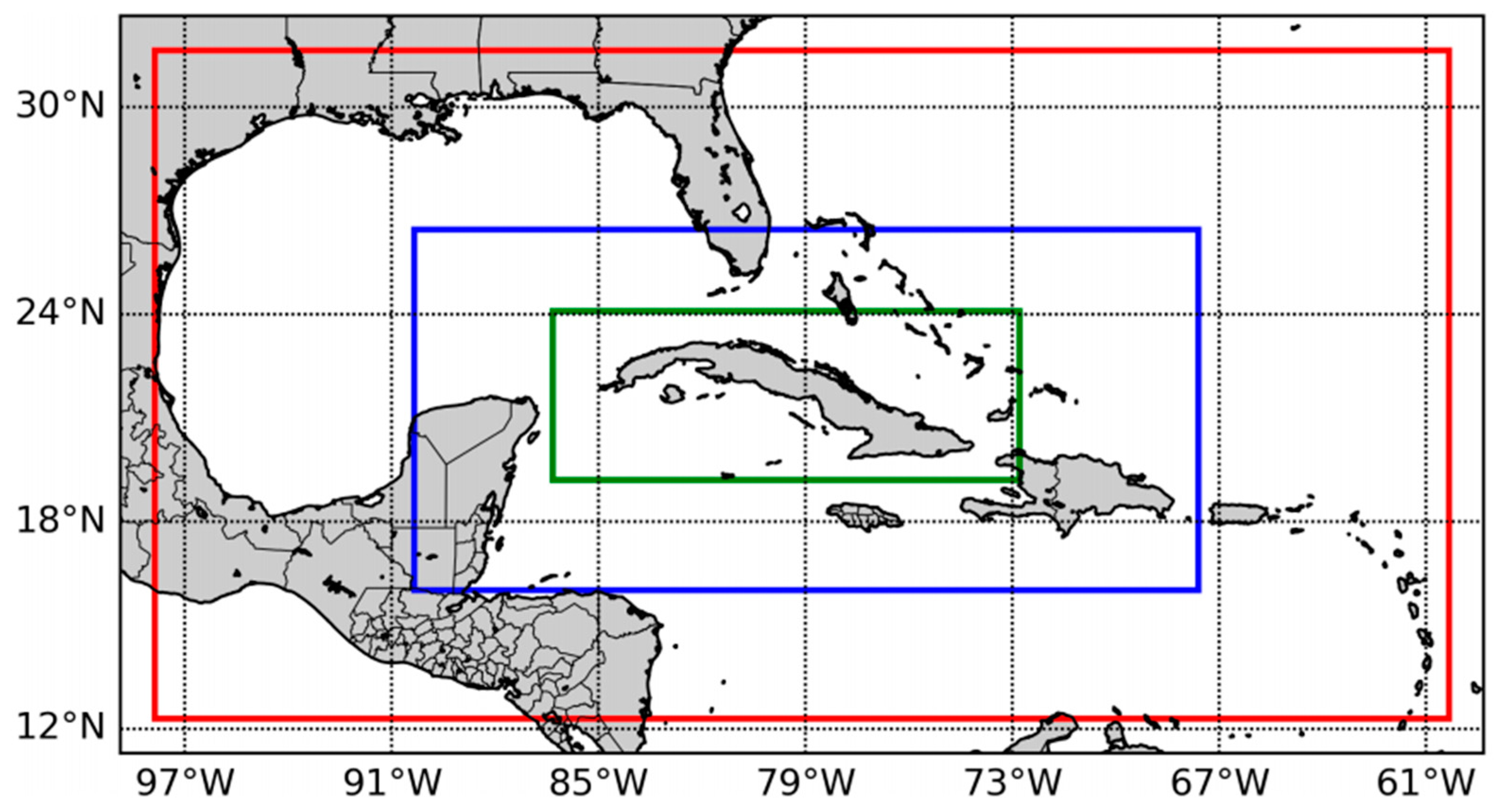
As was mentioned before, a multi-layer perceptron model (MLP) was used in order to extend a previous result in which the observations of meteorological surface stations were used for training. The MLP describes an artificial neural network that uses the output to establish a relationship with the input data. In our case, the input data were the QPF values directly taken from SisPI, and as output the precipitation estimation of GPM was used. The MLP was configured with 64 neurons in the hidden layer and a sigmoid function activation for the hidden and the output layers. The machine learning platform Tensorflow as well as the Keras library [9] were used for implementing the MLP. The training, validation, and verification steps were development using the available data in the period of 2018–2019.

3. Data Used

As observation data for training, the precipitation data from the Global Precipitation Mission was used. In particular, we used GPM_3IMERGHH, which is the GPM IMERG Final Precipitation L3 product (version 06) with a temporal resolution of 30 min and a spatial resolution of 0.1° × 0.1°. This is a multi-satellite precipitation product with global coverage, and it is a Level 3 NASA product that unifies and inter-calibrates data of and about some constellations and types of satellites from several space agencies [10].

The correction using the MLP was applied to the forecast of SisPI over the highest spatial resolution domain (3 km, see Figure 1). SisPI uses the Weather Research and Forecast (WRF) V3.8.1 model [11] as the numerical forecast core initialized with the 0.5 degrees of spatial resolution output of the Global Forecast System (GFS). The main details of the physical configuration are shown in

Table 1. Physical configuration of the WRF used in SisPI (see [11] for the details of each parameterization).

Parameters	Settings
Spatial resolution	Three nested domains of 27, 9, and 3 km of resolution
Nx	145, 162, 469
Ny	82, 130, 184
Nz	28, 28, 28
Domain center	21.8 N, 79.74 W
Time step	150 s
Microphysics	WSM5, WSM5, and double-moment Morrison
Cumulus	Grell–Freitas, Grell–Freitas, and not activated
Long radiation	RRTM scheme: Rapid Radiative Transfer Model
Short radiation	Dudhia scheme: simple downward integration allowing for efficient cloud and clear-sky absorption and scattering
Surface physics	Noah land surface model: unified NCEP/NCAR/AFWA scheme with soil temperature and moisture in four layers, fractional snow cover, and frozen soil physics.
Surface layer	Eta similarity: Used in the Eta model
PBL	Mellor–Yamada–Janjic, Mellor–Yamada–Janjic, and Mellor–Yamada–Janjic

. This system generates 24 forecast hours, updated four times during the day at 0000, 0600, 1200, and 1800 UTC; in this investigation the 0000 UTC initialized forecast is used.

Once the training step was complete, the validation and the verification steps were carried out using the observations of the surface meteorological stations. Figure 2 shows the location of the 67 surface weather stations that were included in this study. A conventional verification process was applied in order to analyze the ability of the MLP to correct the bias. The following statistical metrics were computed: mean absolute error (mae), the mean square error (mse), and Pearson’s correlation coefficient ($p_{corr}$); the cell-point verification approach was applied [12].

4. Results and Discussion

In this section we discuss some preliminary results that show the improvement in the QPF when an ANN model is used as a bias correction method. The analysis is done by taking two study cases: 5 and 10 July of 2019. Rainfall between 4 and 10 July, 2019, was encouraged by the evening instability as a result of the diurnal warming, the sufficient moisture content in the lower troposphere, and conditions in the mesoscale, together with the transit of active tropical waves through the seas at the south of Cuba (http://www.insmet.cu/asp/genesis.asp?TB0=PLANTILLAS&TB1=MES&TB2=/Mes/JULIO2019.HTM&TB3=2019 accessed on 12 January 2020). The reason for selecting these cases is because they are one of the situations in which SisPI frequently fails [6,7].

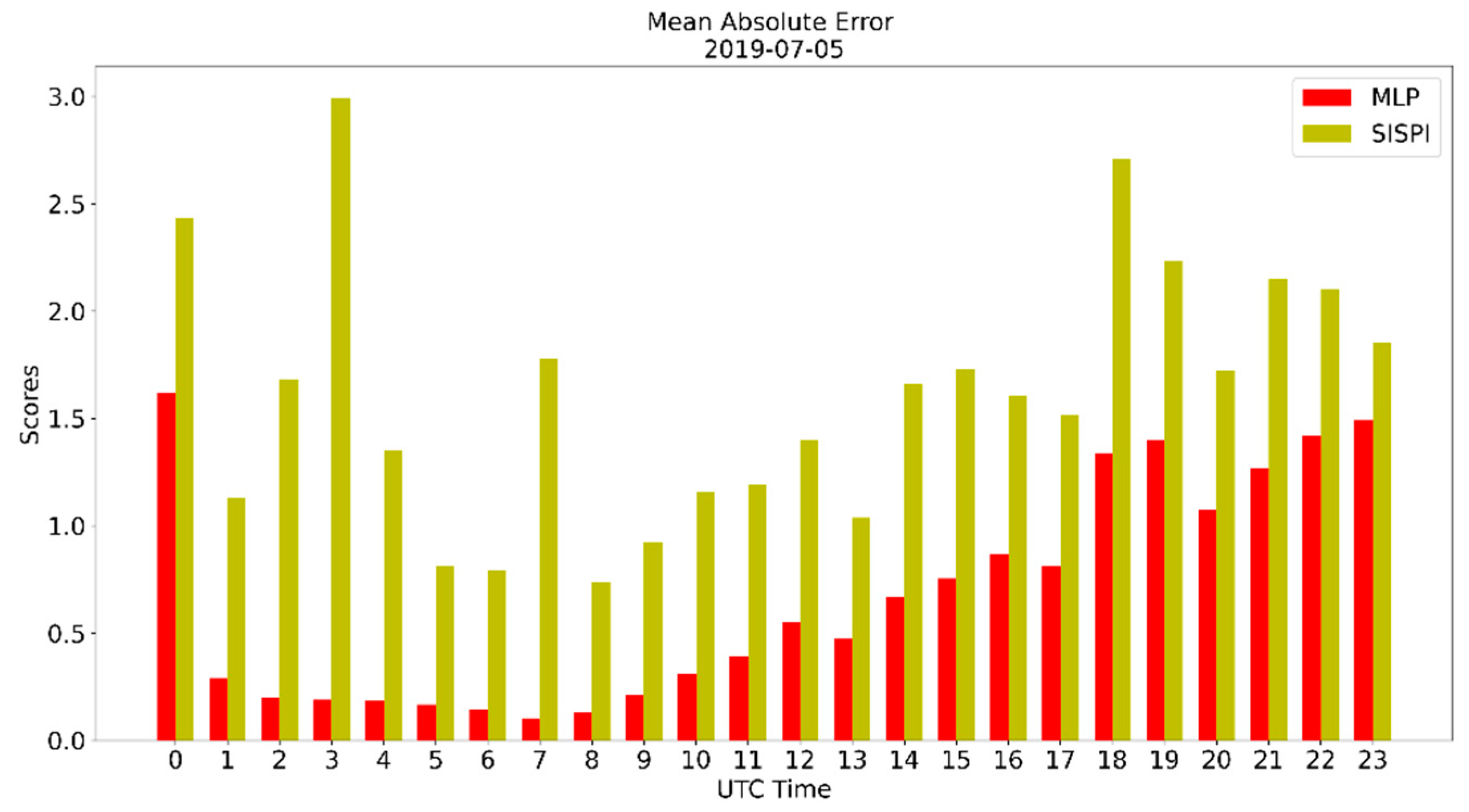
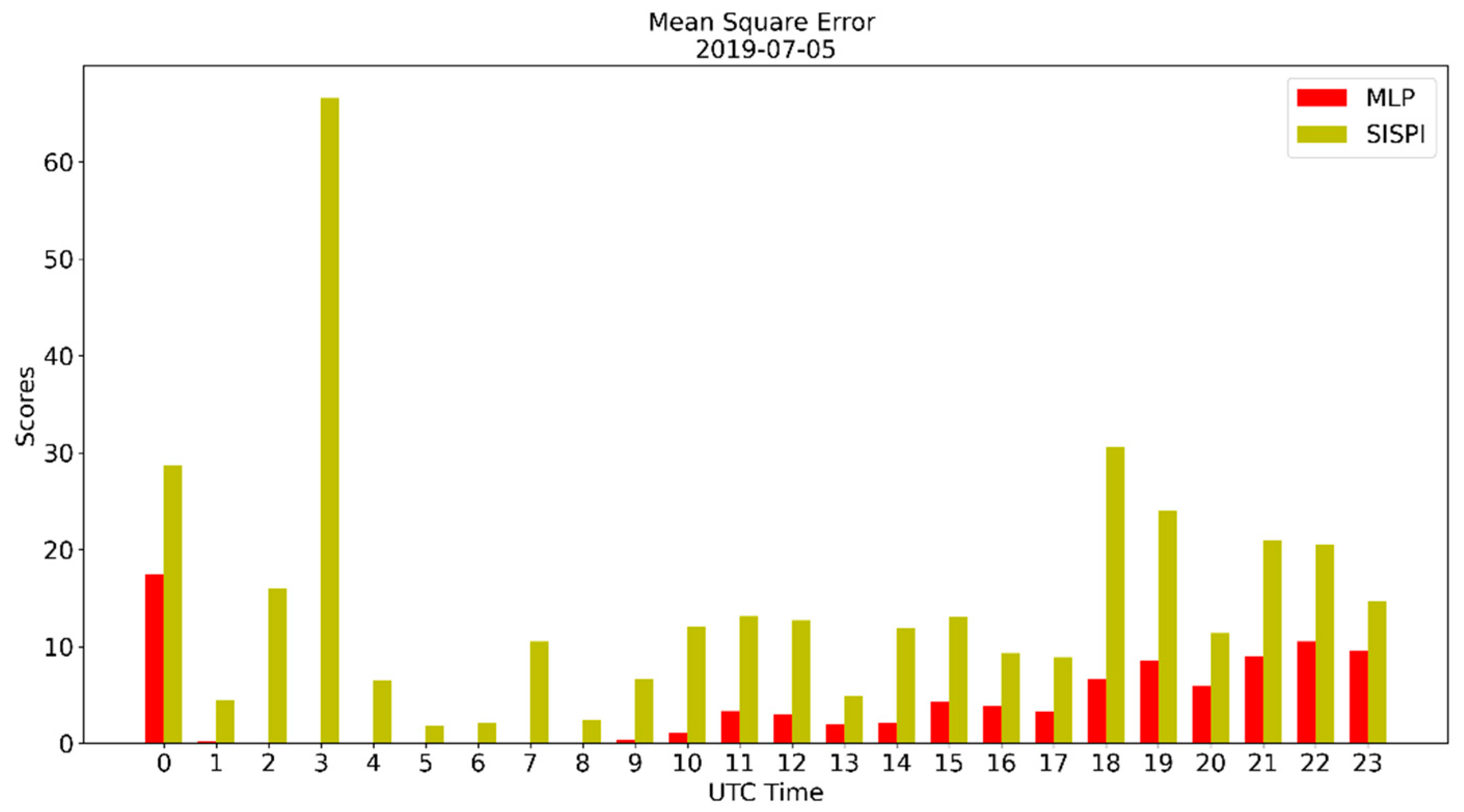
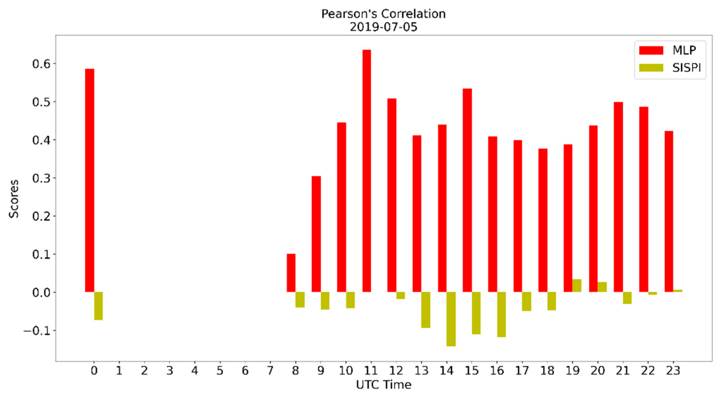
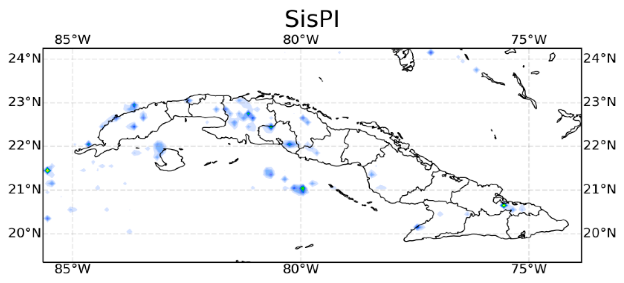
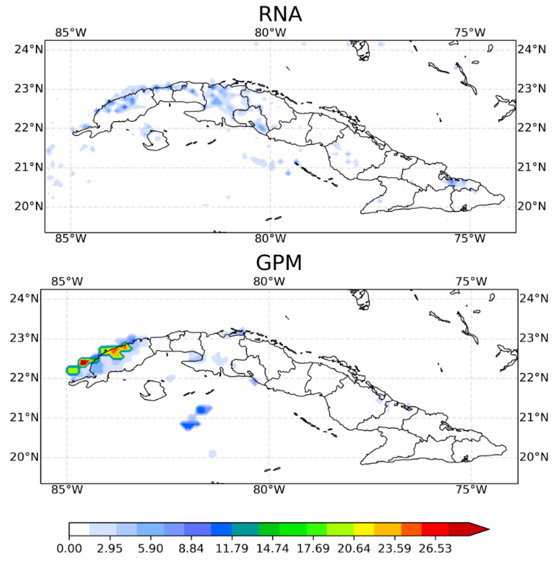
4.1. Case Study 5 July 2019

The mae, mse, and $p_{corr}$ for all forecast times are shown in Figure 3, Figure 4 and Figure 5, respectively. Notice that for the first 7 forecast hours the correction through the MLP model is greater with an error reduction of 2.0 mm/3 h for mae and 60 mm/3 h for mse. In the evening hours, although there is also a decrease in the error values, this decrease is more discreet. This makes sense when one takes into account that, when using SisPI runs initialized at 0000 UTC, the first 7 h of the WRF is in the spin-up period which can extend to the first 12 h of forecasting. Therefore, for this case study, the MLP model constitutes a tool not only to reduce the error, but also to enhance the quality of the forecast in the WRF spin-up period.

The behavior of the correlation curve indicates that the SisPI forecast behaves contrary to what was recorded in the observations. The negative values of $p_{corr}$ suggest that when precipitation was recorded in the surface meteorological station, the SisPI did not predict rain, or it could be the opposite. However, a more rigorous and in-depth study must be done to be able to affirm this behavior. When it comes to very high-resolution forecasts, errors have a double penalty due to position error. Therefore, the fact that SisPI does not predict precipitation at a given point could be due to a position error of the precipitation area. In the case of the correction with the MPL, however, the previous situation is corrected, and the correlation reaches values of up to 0.6, being positive for all forecast periods. In the spin-up hours, $p_{corr}$ is zero since the mean is zero as well.

Figure 6 shows the SisPI forecast, the corrected SisPI forecast, and the GPM precipitation for 1800 UTC. It can be seen that the SisPI forecast underestimates the precipitation over the province of Pinar del Río not only quantitatively but also from a spatial point of view. While the GPM estimate presents values of more than 20 mm/3 h, SisPI barely predicts 11 mm/3 h. On the province of Matanzas the opposite is observed; SisPI suggests the occurrence of rain practically in the entire province, being a false alarm. The correction fails to improve SisPI’s prognosis. Over the province of Pinar del Río, the MLP achieves a better spatial representation of precipitation; however, no improvement is obtained in terms of the quantitative forecast of precipitation. Furthermore, the MLP fails to eliminate false alarms.

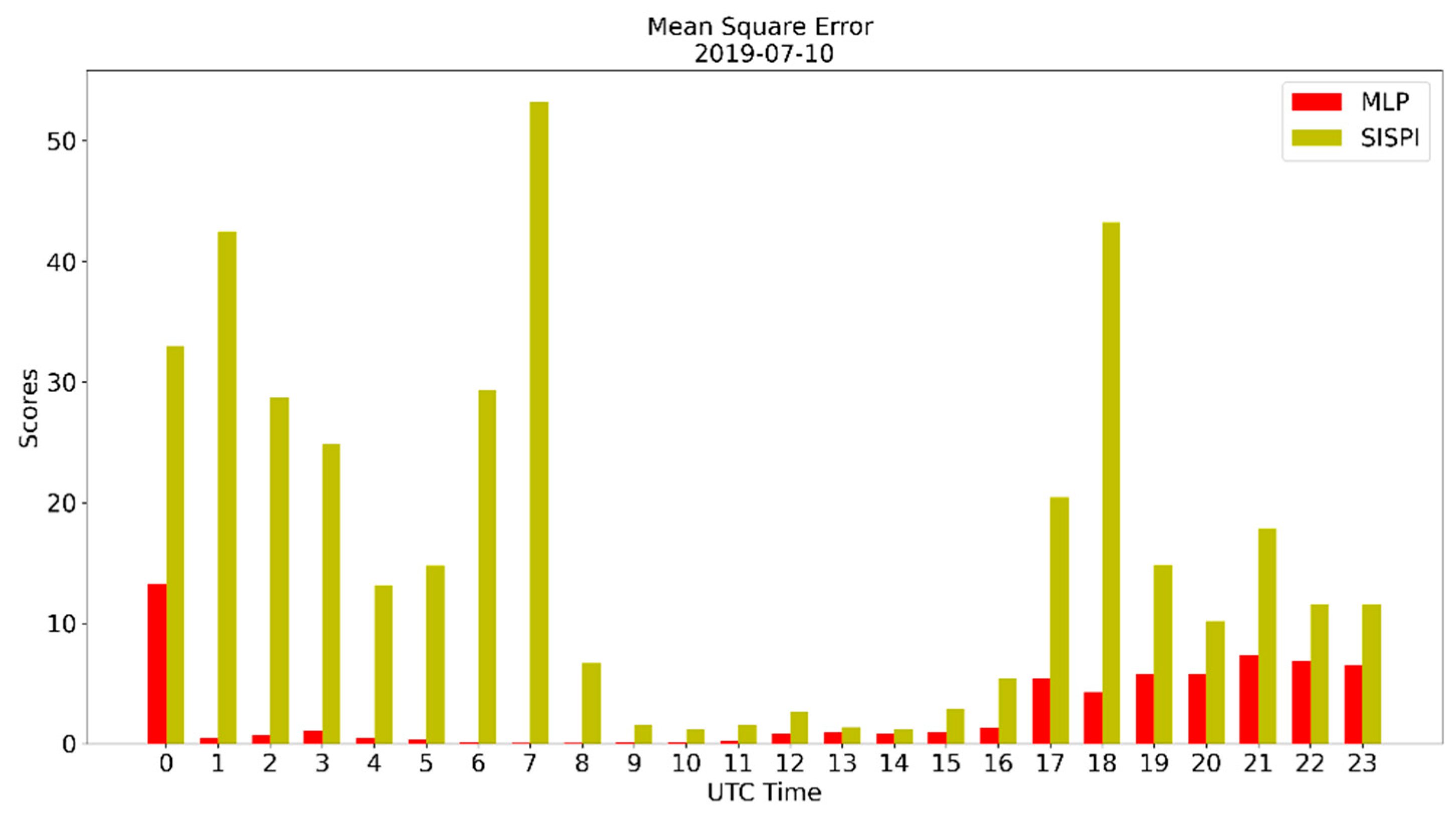
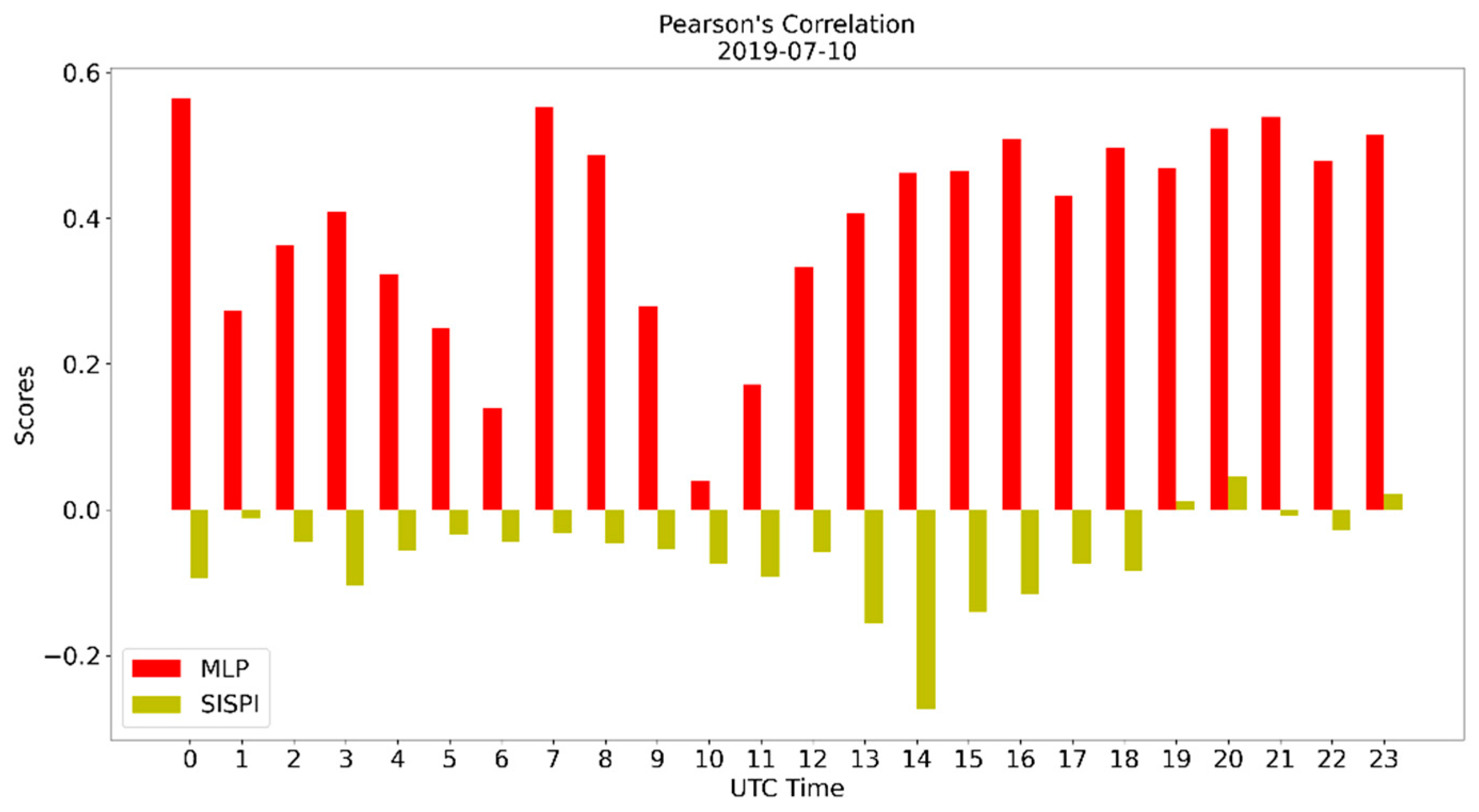
4.2. Case Study 10 July 2019

A similar behavior of mae, mse, and $p_{corr}$ is observed for this case study (Figure 7, Figure 8 and Figure 9, respectively). As before, during the spin-up time, the MLP correction shows its ability to reduce the WRF error.

According to the GPM estimate (Figure 10 bottom panel), at 2200 UTC, non-significant values between 6 mm/3 h and 12 mm/3 h occurred over the provinces of Pinar del Río, Artemisa, Havana, Camaguey, and Holguín. SisPI, however, predicts more than 30 mm/3 h in the northern region of Matanzas, which is considered a false alarm. In the rest of the country there is also an overestimation of precipitation values. In this forecast period, the application of the MLP failed to correct any of the errors indicated above and increased the spatial overestimation of precipitation. The above indicates that there is still much work to be done, and that other ANN models with more appropriate characteristics for this type of application should be explored, such as convolutional networks, for example.

5. Conclusions

The research presented consists of an application of a multi-layer perceptron artificial neural network for the bias correction of QPF. Some positive results were obtained in terms of the reduction of the metrics mae and mse, the correction being better in the spin-up period of the WRF. However, the MLP model was not able to overcome quantitative and positional errors when looking at a given forecast timeframe. It is recommended to extend the experiments to more appropriate ANN models for correcting the quantitative forecast of precipitation, taking into account its value and also the spatial location.

References

1. Bishop, C.M. Neural Networks for Pattern Recognition; University Press: Oxford, UK, 1995. [Google Scholar]
2. Haykin, S. Neural Networks: A Comprehensive Foundation, 2nd ed.; Prentice Hall: New York, NY, USA, 1998. [Google Scholar]
3. Hsieh, W.W.; Tang, B. Applying neural network models to prediction and data analysis in meteorology and oceanography. Bull. Am. Meteorol. Soc. 1998, 79, 1855–1870. [Google Scholar] [CrossRef]
4. Sanaz, M. Bias Correction of Global Circulation Model Outputs Using Artificial Neural Networks; Georgia Institute Technology: Atlanta, GA, USA, 2015. [Google Scholar]
5. Fuentes-Barrios, A.; Sierra-Lorenzo, M.; Morfa-Ávalos, Y. Corrección del pronóstico cuantitativo de laprecipitación mediante el uso de redes neuronales. Revista Cubana de Meteorología 2020, 26, 3. [Google Scholar]
6. Sierra-Lorenzo, M.; Ferrer-Hernández, A.L.; Hernández-Valdés, R.; González-Mayor, Y.; Cruz-Rodríguez, R.C.; Borrajero-Montejo, I.; Rodríguez-Genó, C. Sistema Automático de Predicción a Mesoescala de Cuatro Ciclos Diarios; Technical Report; Instituto de Meteorología de Cuba: La Habana, Cuba, 2014. [Google Scholar]
7. Sierra-Lorenzo, M.; Borrajero-Montejo, I.; Ferrer-Hernández, A.L.; Hernández-Valdés Morfa-Ávalos, Y.; Morejón-Loyola, Y.; Hinojosa-Fernández, M. Estudios de Sensibilidad del Sispi a Cambios de la pbl, la Cantidad de Niveles Verticales y, las Parametrizaciones de Microfısica y Cúmulos, a muy alta Resolución; Technical Report; Instituto de Meteorología de Cuba: La Habana, Cuba, 2017. [Google Scholar]
8. SisPI. 2021. Available online: http://modelos.insmet.cu/sispi/ (accessed on 15 January 2020).
9. Buhigas, J. Everything you need to know about TensorFlow, Google’s Artificial Intelligence platform. Digit. Bridges 2018, 2, 14. [Google Scholar]
10. Hou, A.Y.; Kakar, R.K.; Neeck, S.; Azarbarzin, A.A.; Kummerow, C.D.; Kojima, M.; Oki, R.; Nakamura, K.; Iguchi, T. The Global Precipitation Measurement Mission. Bull. Am. Meteorol. Soc. 2014, 95, 701–722. [Google Scholar] [CrossRef]
11. Mesoescale & Microescale Meteorology Division. ARW Version 3 Modeling System User’s Guide; Complementary to the ARW Tech Note; NCAR: Boulder, CO, USA, 2014; p. 141. Available online: http://www2.mmm.ucar.edu/wrf/users/docs/userguideV3/ARWUsersGuideV3.pdf (accessed on 15 January 2020).
12. WWRP/WGNE Joint Working Group on Verification. Forecast Verificacion-Issues, Methods and FAQ (pdf Version). 2008. Available online: http://www.cawcr.gov.au/staff/eee/verif/verif_web_page.html (accessed on 15 May 2020).
Figure 1. Simulation domains for SisPI. The green square corresponds with the 3 km resolution domain used in this study.
Environsciproc 08 00038 g001
Figure 2. Location of the meteorological surface stations.
Environsciproc 08 00038 g002
Figure 3. Mean absolute error of the SisPI forecast for 5 July 2019 and the SisPI forecast after bias correction with the MLP model.
Environsciproc 08 00038 g003
Figure 4. Mean square error of the SisPI forecast for 5 July 2019 and the SisPI forecast after bias correction with the MLP model.
Environsciproc 08 00038 g004
Figure 5. Pearson’s correlation of the SisPI forecast for 5 July 2019 and the SisPI forecast after bias correction with the MLP model.
Environsciproc 08 00038 g005
Figure 6. SisPI precipitation forecast (top panel), MLP correction (middle panel) and precipitation estimated by GPM product (bottom panel) for 5 July 2019 at 1800 UTC.
Environsciproc 08 00038 g006aEnvironsciproc 08 00038 g006b
Figure 7. Mean absolute error of the SisPI forecast for 10 July 2019 and the SisPI forecast after bias correction with the MLP model.
Environsciproc 08 00038 g007
Figure 8. Mean square error of the SisPI forecast for 10 July 2019 and the SisPI forecast after bias correction with the MLP model.
Environsciproc 08 00038 g008
Figure 9. Pearson’s correlation of the SisPI forecast for 10 July 2019 and the SisPI forecast after bias correction with the MLP model.
Environsciproc 08 00038 g009
Figure 10. SisPI precipitation forecast (top panel), MLP correction (middle panel) and precipitation estimated by GPM product (bottom panel) for 10 July 2019 at 2200 UTC.
Environsciproc 08 00038 g010aEnvironsciproc 08 00038 g010b