Next Article in Journal
Geological Materials as Cultural Markers of Water Resources
Previous Article in Journal
Estimation of Surface Soil Moisture at the Intra-Plot Spatial Scale by Using Low and High Incidence Angles TerraSAR-X Images
 
 
Please note that, as of 4 December 2024, Environmental Sciences Proceedings has been renamed to Environmental and Earth Sciences Proceedings and is now published here.
Proceeding Paper

Development of Prediction Model for Storm Surge Hazards in the Developing Countries †

1
Department of Mathematics and Natural Sciences, Brac University, 66 Mohakhali, Dhaka 1212, Bangladesh
2
Department of Mathematics, University of Rajshahi, Rajshahi 6205, Bangladesh
*
Author to whom correspondence should be addressed.
Presented at the 3rd International Electronic Conference on Geosciences, 7–13 December 2020; Available online: https://iecg2020.sciforum.net.
Environ. Sci. Proc. 2021, 5(1), 7; https://doi.org/10.3390/IECG2020-08630
Published: 30 November 2020

Abstract

:
Bangladesh is one of the most vulnerable countries in the world with around 718,000 deaths in the past fifty years. This country is especially in danger for cyclones because of its location in the triangular-shaped Bay of Bengal. The scientific scenario suggests that enlarged sea surface temperature will intensify cyclone movement. Tropical cyclones generate storm surges. Storm surges severely change the coastal environment, damage coastal structures, destroy forests and crops, inundate the coastline with saltwater and cause loss of lives. Due to overcrowding in the mainland in Bangladesh, poor and landless people live on the coast and they face frequent cyclones and associated surges. They affect food and drinking water and there is danger of transmission risks of infectious diseases, such as diarrhea, malaria, eye infections, skin diseases, etc. Some problems following a cyclone are usually created for their low literacy rate and poor knowledge of the environment. The tangible monitoring and warning of cyclones and associated surges should be given more priority for the region. The main objectives of this paper are to highlight the existing activities of the model in storm surges and related areas in the Bay of Bengal. We will explain the progress of a location-specific real-time standpoint prediction system for providing effective and timely surge forecasts. We will also introduce a model through numerical experiments using a severe cyclone in April 1991 to predict the storm surges that will be used to reduce economic losses and the number of deaths during a strong storm surge in the coastal area of Bangladesh.

1. Introduction

Storm surges are associated with severe weather such as tropical cyclones that constitute the world’s most catastrophic natural disasters [1]. Among the most threatening calamities, storm surges stand out as the most damaging and undoubtedly as a cause of death and ruin as massive as that of earthquakes and tsunamis [2]. In history, low-lying deltaic regions of Bangladesh and Myanmar are heavily subjected to storm surge hazards. Fortunately, in most recent storm surge cases, the death toll is not as high as previously since the storm surge warning systems in fact worked well. However, we keep in mind that storm surges could be a cause of high death rates in the future while the number of residents is rising in coastal regions [3,4]. The key components contributing to calamitous surges in Bangladesh are as follows [5]:
Convergence of the Bay
High astronomical tides
Positive cyclone track
Shallow coastal water
Densely populated low-lying island.
An updated and accurate storm surge prediction system is required to mitigate and prevent coastal disasters. It is essential to study local allocation characteristics exclusively along with previous storm surge heights in order to update the numerical forecast systems. Various ranges of motion must be investigated through numerical discrete structure of the governing equations to forecast surges in coastal areas exactly. It is also indispensable to examine long-term observation data perfectly in predicting the areas that storm surges might affect with precision [6,7,8]. As the landward boundary is approached, substantial grid refinement is typically required to resolve important schemes and prevent energy from aliasing. In providing an adequate resolution in the near shore region without increasing the size of the discrete problem, a numerical method must be used that permits a very high degree of grid flexibility.

2. Materials

2.1. Model Equation

The following depth-averaged vertically integrated form of the mass conservation equation, and the x and y components of the momentum equation, respectively, are used in investigating the dynamical process in the sea [6]:
ξ t + x [ ( ζ + h ) u ] + y [ ( ζ + h ) v ] = 0 ,
u t + u u x + v u y f v = g ξ x + T x ρ ( ξ + h ) C f u ( u 2 + v 2 ) 1 / 2 ξ + h ,
v t + u v x + v v y + f u = g ξ y + T y ρ ( ξ + h ) C f v ( u 2 + v 2 ) 1 / 2 ξ + h .
In Equations (1)–(3), x and y are coordinate axes directed towards the south and east, respectively, where the origin is set at the northwest corner ( 23 N , 85 E ) of the computational x y -plane (Figure 1); u and v represent Reynold’s averaged components of velocity in the x and y directions, respectively; ζ ( x , y , t ) is the displaced level of free surface of water above or below the mean sea level (MSL); h ( x , y ) is the undisturbed water depth; f ( = 2 Ω sin φ , where Ω is the angular speed of the earth rotation about its own axis, and φ represents the latitude of a position of interest) is the Coriolis parameter; g (=9.81 m/s2) is the acceleration due to local gravity; ρ is the sea water density, assumed to be uniform; C f (=0.0026) is the dimensionless bottom friction coefficient; T x and T y are the x and y components, respectively, of the wind stress acting on the sea surface.
The wind stress components mentioned above are derived following Ali [5] as
T x , T y = ρ a C D u a 2 + v a 2 1 / 2 u a , v a .
To derive the components of the wind stress, wind field is required. As in [7], the wind field is generated through the following formula:
v a = V o r a / R 3 , for r a R V o R / r a 3 , for r a > R
In Equations (4) and (5), u a and v a stand for the x and y components of the surface wind, respectively, ρ a is the air density, C D (= 0.0028) is the surface drag coefficient, V 0 is the maximum sustained wind at the maximum radial distance R and r a is the distance between the cyclone center and the point at which the wind field is desired.

2.2. Boundary Conditions

The study domain has three open boundaries and one closed boundary. At the closed boundary (coastal or island boundary), the normal component of the depth averaged velocity is set to zero. Following Paul et al. [6], the western, eastern and southern open boundary conditions are, respectively, taken into account. These lead to
v + g / h 1 / 2 ζ = 0 ,   v g / h 1 / 2 ζ = 0 ,   u g / h 1 / 2 ζ = 2 a g / h 1 / 2 sin 2 π t T + ϕ ,
where a , T , and ϕ stand for, respectively, the amplitude, period and phase of the tidal constituent under consideration.
Meghna River mouth is considered as open boundary and the freshwater discharge through the river is considered following Roy [7]. This leads to
u b = u + Q B h + ξ ,
where Q denotes the volume of freshwater river discharge in a unit time and B represents its width.

2.3. Input

In our study, we need several types of input. The meteorological input, namely maximum sustained wind radius, maximum sustained wind speed and storm track information are obtained from the Bangladesh Meteorological Department (BMD) through personal communication. The time varying positions of the storm and its nature are presented in Table 1 for a better understanding. The study also needs bathymetry data which is collected from the British Admiralty Chart. Shepard interpolation is used to supply water depth at the grid points of the three schemes, as we will see later, representing water. Further, the study needs tidal constants to generate a tidal response on the area of interest, which are taken from the study due to Paul et al. [6]. Following Paul et al. [9], the freshwater discharge through the river per unit time is taken as Q = 5100   kg / s and the remaining parameters have been assumed to have their standard value.

3. Methodology

3.1. Numerical Procedures

3.1.1. Set-Up of Nested Scheme

In order to incorporate the coastal complexity with minimum cost, a nested grid technique is used in this study. A high-resolution fine grid model, referred to as FMS, is nested into a scheme with relatively low resolution, which is referred to as CMS. It is of interest to note here that the FMS is designed to incorporate all the major offshore islands along the coast of Bangladesh. Now to incorporate properly the land-sea interface and bottom topographic detail of the Meghna estuarine area, which is referred to as the world’s most vulnerable zone, a scheme with very high resolution is nested into the FMS. The innermost scheme is referred to as VFMS. To have a clear idea about the schemes, Figure 1 and Table 2 are inserted for a better perspective. It is to be noted here that Paul et al. [6] first used the MOL to solve shallow water equations in predicting water levels due to the tide-surge interaction along the coast of Bangladesh, where they used a nested grid technique without high resolution of grids. Thus, this study is an improvement on that of Paul et al. [6].

3.1.2. Discretization

The aim of the study is to solve the governing equations with a numerical method of lines (MOL). It is of interest to note here that the method is efficient over the standard finite difference method due to having some benefits, especially, in computational coast, stability criterion, and simplicity in solving partial differential equations. Thus, in this regard, the equations and the boundary conditions are discretized only for spatial derivatives/variables by means of a semi-implicit three point central finite difference technique. We consider the discrete points in the xy-plane by defining x i = ( i 1 ) Δ x , i = 1 , 2 , 3 , , M (even), y j = ( j 1 ) Δ y , j = 1 , 2 , 3 , , N   ( odd ) .
If any dependent variable ξ ( x , y , t ) at a grid point ( x i , y j ) at time t k is represented by ξ ( x i , y j , t k ) = ξ i , j k , then with the aid of the notations 0.5 ( ξ i + 1 , j k + ξ i 1 , j k ) = ξ i , j k ¯ x , 0.5 ( ξ i , j + 1 k + ξ i , j 1 k ) = ξ i , j k ¯ y and 0.25 ( ξ i + 1 , j k + ξ i 1 , j k + ξ i , j + 1 k + ξ i , j 1 k ) = ξ i , j k ¯ x y , one can discretize the equations of interest as follows.
For every grid point ( x i , y j ) , where i = 2 , 4 , 6 , , M 2 and j = 3 , 5 , 7 , , N 2 , Equation (1) can be written as
ζ t i , j = f 1 ζ l , m k , u l , m k , v l , m k , h l , m = C R 1 + C R 1 ,
where l = i 1 , i , i + 1 ; m = j 1 , j , j + 1 ;
C R 1 = ζ i + 1 , j k ¯ x + h i + 1 , j u i + 1 , j k ( ζ i 1 , j k ¯ x + h i1, j ) u i1, j k 2 Δ x ,   CR2= ( ζ i,j+ 1 k ¯ y + h i,j+1 ) v i,j+1 k ( ζ i,j1 k ¯ y + h i,j1 ) v i,j1 k 2Δy .
Again, for every point ( x i , y j ) , where i = 3 , 5 , 7 , , M 1 and j = 3 , 5 , 7 , , N 2 , Equation (2) can be written as
u t i , j = f 2 ξ l , m k + 1 , u l , m k , v l , m k , h l , m = U R 1 + U R 2 + U R 3 + U R 4 + U R 5 + U R 6 ,
where l = i 2 , i 1 , i , i + 1 , i + 2 ; m = j 2 , j 1 , j , j + 1 , j + 2 ;
UR1= u i,j k u i+2,j k u i2,j k 4 Δ x , for   im1 u i,j k 0.5 3 u i,j k u i2,j k u i2,j k 4 Δ x , for   i=m1 ,   UR2= v i,j k ¯ xy u i,j+1 k ¯ y u i,j1 k ¯ y 2 Δy ,   UR3= f i,j v i,j k ¯ xy , UR4= g ζ i+1,j k+1 ζ i1,j k+1 2 Δx ,   UR5= T x ρ ( ζ i,j k+1 ¯ x + h i,j ) ,   UR6= C f u i,j k ζ i,j k+1 ¯ x + h i,j + [ u i,j k 2 + ( v i,j k ¯ xy ) 2 ] 1/2 ,
Finally, for every grid point ( x i , y j ) , where i = 2 , 4 , 6 , , M 2 and j = 2 , 4 , 6 , , N 1 , Equation (3) can be written as
v t i , j = f 3 ξ l , m k + 1 , u l , m k , v l , m k , h l , m = V R 1 + V R 2 + V R 3 + V R 4 + V R 5 + V R 6 ,
where l = i 2 , i 1 , i , i + 1 , i + 2 ; m = j 2 , j 1 , j , j + 1 , j + 2 ;
V R 1 = u i , j k ¯ x y v i + 1 , j k ¯ x v i 1 , j k ¯ x 2Δx , for   i 2 u i,j k ¯ x y v i + 1 , j k ¯ x 0.5 3 v i,j k v i+2,j k 2Δx , for  i= 2 V R 2 = v i , j k v i , j + 2 k v i , j 2 k 4Δy , for   j 2 , j n 1 v i,j k v i , j + 2 k 0.5 3 v i,j k v i,j+2 k 4Δy , for   j= 2 v i,j k 0.5 3 v i,j k v i,j2 k v i,j2 k 4Δy , for   j = n 1 , V R 3 = f i,j u i,j k ¯ xy ,   V R 4 = g ζ i,j+1 k +1 ζ i,j1 k +1 2 Δy ,   VR5= T y ρ ( ζ i,j k+1 ¯ y + h i,j ) ,   VR6= C f v i,j k ζ i,j k+1 ¯ y + h i,j [ u i,j k ¯ x y 2 + ( v i,j k ) 2 ] 1/2 .
The boundary conditions specified by Equation (6), the elevations at j = 1 (eastern boundary), j = N (western boundary and i = M   ( southernboundary ) are computed in the following manner, respectively:
ζ i , 1 k + 1 = ζ i , 3 k + 1 2 ( h i , 2 / g ) V i , 2 k
ζ i , N k + 1 = ζ i , N 2 k + 1 + 2 ( h i , N 1 / g ) V i , N 1 k ,
ζ M , j k + 1 = ζ M 2 , j k + 1 + 2 ( h M 1 , j / g ) U M 1 , j k + 4 a sin 2 π k Δ t / T + ϕ ,
where i = 2 , 4 , 6 , , M 2 and j = 1 , 3 , 5 , , N .
The freshwater Meghna River discharge is incorporated through Equation (7), where the velocity component Ub is calculated at ( 1 , j ) , j = 7 , 9 , 11 , , 19 in the following manner:
( U b ) 1 . j k + 1 = ( U b ) 3 , j k + 1 + Q ( ζ 1 , j k + 1 + h 1 , j ) B

3.1.3. Working Procedure and Model Run

Discretized form of Equations (8)–(10) are available in [6]. However, briefly they are inserted here for a better understanding. First Equation (8) is solved with RK(4,4) method for the elevation ζ at the internal (even, odd) grid points representing water of the CMS. Discretized BCs given by Equations (11)–(13) are then used to estimate ζ at the boundary (even, odd) grid points. An interpolation is then adopted to obtain ζ at the leftover grid points representing water and the land-sea interface. The wind field is then generated using Equations (4) and (5). Then Equation (9) is used for estimating u at the interior (odd, odd) grid points representing water by inserting the parametric values involved and finally v is evaluated in a similar fashion at the interior (even, even) grid points solving Equation (10). After computing ζ , u , and v in the CMS, the scheme is coupled with the FMS following a process found in [6] to have the boundary values from the CMS to run the FMS. In a similar manner, the VFMS is run with the boundary information from the FMS. Along the northern open boundary segment, U b is taken into account for the VFMS using Equation (14). This process is repeated over time providing the updated values of ζ , u and v as initial conditions for computing WLs () owing to tide, surge and nonlinear interaction of tide and surge. For computing tide, surge and total water levels (water levels due to tide-surge interaction) all the models, namely tide, surge, and tide–surge interaction were run considering the time step as Δ t = 60 s to ensure Courant–Friedrich–Lewy (CFL) stability criterion. It is noteworthy that our model can run individually and simultaneously. The first tide model was run from the cold start ( ζ = 0 , u = 0 , v = 0   at   t = 0 ) to get water levels with respect to the mean sea levels (MSL) considering the effect of M 2 tidal constituent along the southern open boundary of the CMS in the absence of meteorological forcing. A stable tidal oscillation was obtained after four tidal cycles of integration that provided the profile of the sea surface if the cyclone is not taken into account. In getting the pure surge level, the surge model (in absence of astronomical tide) was also run from the cold start. In achieving total WLs (due to the dynamic interaction of tide and surge), the tide model was run first. After having a stable tidal regime, the surge model was then made to run over it.

4. Results and Discussion

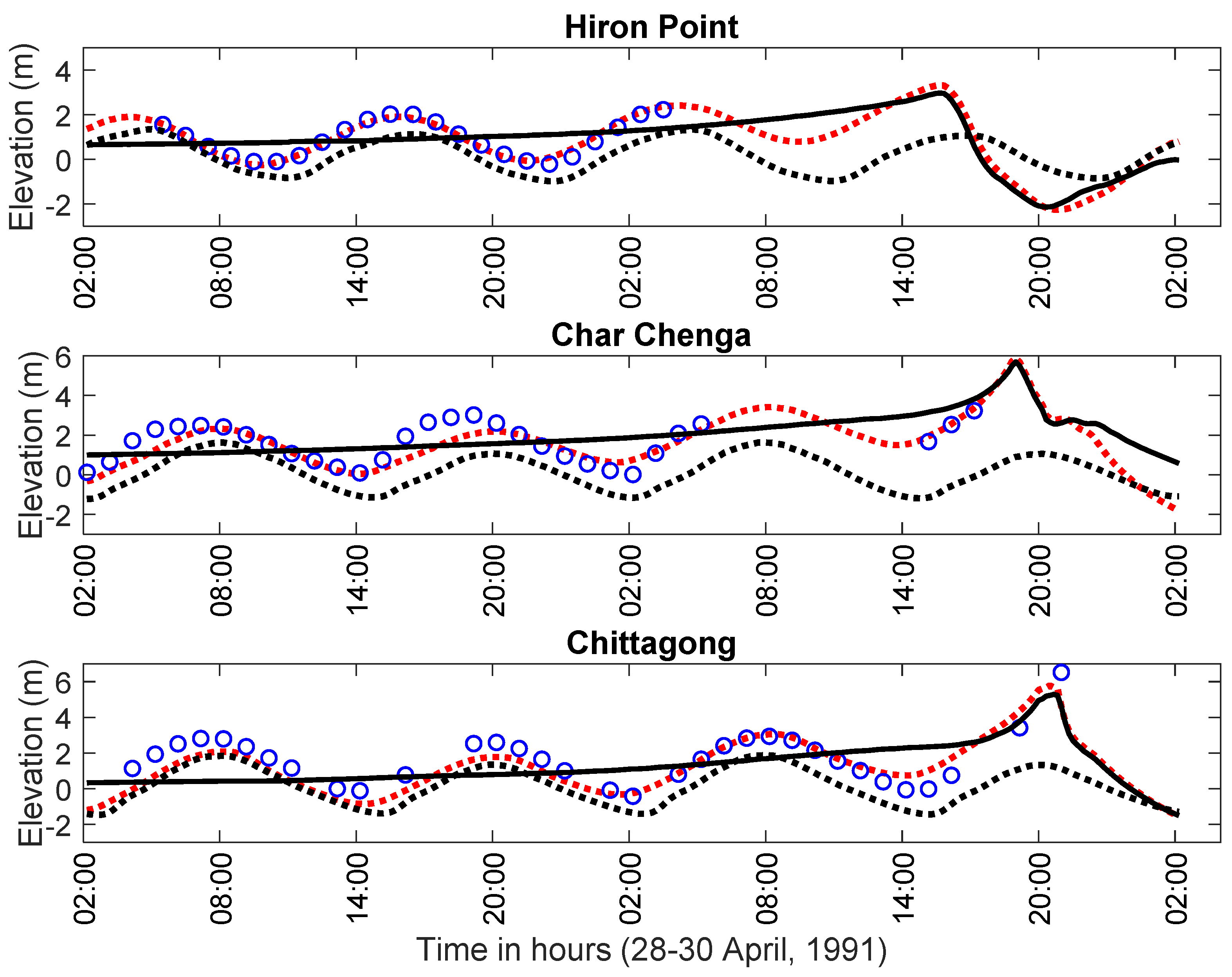
Water levels due to tide, surge and their interaction are calculated at the stations shown in Figure 1, but for the sake of brevity, the peak water levels due to surge and interaction of tide and surge are presented in Table 3 and the computed time series of water levels due to the tide, surge and the interaction of tide and surge are presented in Figure 2 with observed data. It is seen from Table 3 that our computed peak surge levels (water levels due to meteorological forcing only) along the region of interest vary between 2.97–6.51 m with 5.29 m at Chittagong. Paul et al. [6] predicted 3.52–6.70 m surge along the coast of Bangladesh. Further, according to BMD, the peak surge at Chittagong at the time of landfall was 5.50 m. Thus, our computed surge level agrees well with the reported data by BMD at Chittagong and the simulated surge levels by Paul et al. [6]. Again, our computed peak total water levels were found to vary between 3.86 m (Kuakata) and 7.28 m (Companigonj), which agree fairly well with the results obtained in Paul et al. [6] (see Table 3).
Our computed time series of water levels with respect to the MSL due to tide, surge and the interaction of tide and surge associated with the storm in April 1991 at Hiron Point, Char Chenga (Hatiya) and Chittagong are displayed in Figure 2. The corresponding observed data collected from Bangladesh Inland Water Transport Authority (BIWTA) are also presented in Figure 2. It is seen from Figure 2 that when the surge is away from the coast, the tide dominates the surge level; whether the opposite characteristics can be found when the surge is nearer to the coast as is expected. However, it is perceived from Figure 2 that our computed water levels due to the interaction of tide and surge are in good agreement with the data obtained from BIWTA.
For validation of our simulated results, the root mean square analysis is carried out between the results attained in the study and observed data from BIWTA. The results that came out in this regard are presented in Table 4. The root mean square error (RMSE) values obtained in this regard due to Paul et al. [9] are also presented in the same table for comparison. It is seen from Table 4 that the results attained by the study are considerable and comparable with those presented in [9].

5. Conclusions

In this study, the MOL in coordination with the RK (4,4) method is used to solve vertically integrated shallow water equations in Cartesian coordinates for simulating water levels along the coast of Bangladesh. The water levels due to the non-linear interaction of tide and surge associated with the cyclone in April 1991 are found to be in reasonable agreement with observed data from BIWTA on the basis of RMSE values. The outcome of this study thus can be utilized in practical forecasting.

Author Contributions

H.N. and G.C.P. conceived and designed the experiments and also analyzed the data. H.N. and G.C.P. completed the writing of the manuscript by sharing their knowledge and ideas and polished the paper through double checking. All authors have read and agreed to the published version of the manuscript.

Funding

This research received no external funding.

Institutional Review Board Statement

Not applicable.

Informed Consent Statement

Not applicable.

Data Availability Statement

The data were collected from Bangladesh meteorological Department and Bangladesh Inland Water Transport Authority.

Acknowledgments

Authors would like to articulate their heartfelt thanks to the Department of Mathematics and Natural Sciences, Brac University, Dhaka, Bangladesh for providing suitable research facilities. Moreover, authors take pleasure in expressing their genuine appreciation to the anonymous referees for their significant comments and suggestions.

Conflicts of Interest

The authors declare no conflict of interest.

References

  1. Dube, S.K.; Rao, A.D.; Sinha, P.C.; Murty, T.S.; Bahulayan, N. Storm surge in the Bay of Bengal and Arabian Sea the problem and its prediction. Mausam 1997, 48, 283–304. [Google Scholar] [CrossRef]
  2. Li, J.; Nie, B. Storm surge prediction: Present status and future challenges. Procedia IUTAM 2017, 25, 3–9. [Google Scholar] [CrossRef]
  3. Kohno, N.; Dube, S.K.; Entel, M.; Fakhruddin, S.H.M.; Greenslade, D.; Leroux, M.D.; Thuy, N.B. Recent progress in storm surge forecasting. Trop. Cyclone Res. Rev. 2018, 7, 128–139. [Google Scholar]
  4. Lynch, D.R. Progress in hydrodynamic modeling, review of U.S. contributions, 1979–1982. Rev. Geophys. Space Phys. 1983, 21, 741–754. [Google Scholar] [CrossRef]
  5. <sc>Ali, A. Storm Surges in the Bay of Bengal and Some Related Problems. Ph.D. Thesis, University of Reading, Reading, UK, 1979; p. 227. [Google Scholar]
  6. Paul, G.C.; Ismail, A.I.M.; Karim, M.F. Implementation of method of lines to predict water levels due to a storm along the coastal region of Bangladesh. J. Oceanography 2014, 70, 199–210. [Google Scholar] [CrossRef]
  7. Roy, G.D. Estimation of expected maximum possible water level along the Meghna estuary using a tide and surge interaction model. Environ. Int. 1995, 21, 671–677. [Google Scholar] [CrossRef]
  8. Naher, H.; Paul, G.C. Further Development of Forecasting Model for Storm Surge Hazard along the Coast of Bangladesh. Am. J. Environ. Prot. 2019, 7, 52–55. [Google Scholar]
  9. Paul, G.C.; Ismail, A.I.M.; Rahman, A.; Karim, M.F.; Hoque, A. Development of tide–surge interaction model for the coastal region of Bangladesh. Estuaries Coasts 2016, 39, 1582–1599. [Google Scholar] [CrossRef]
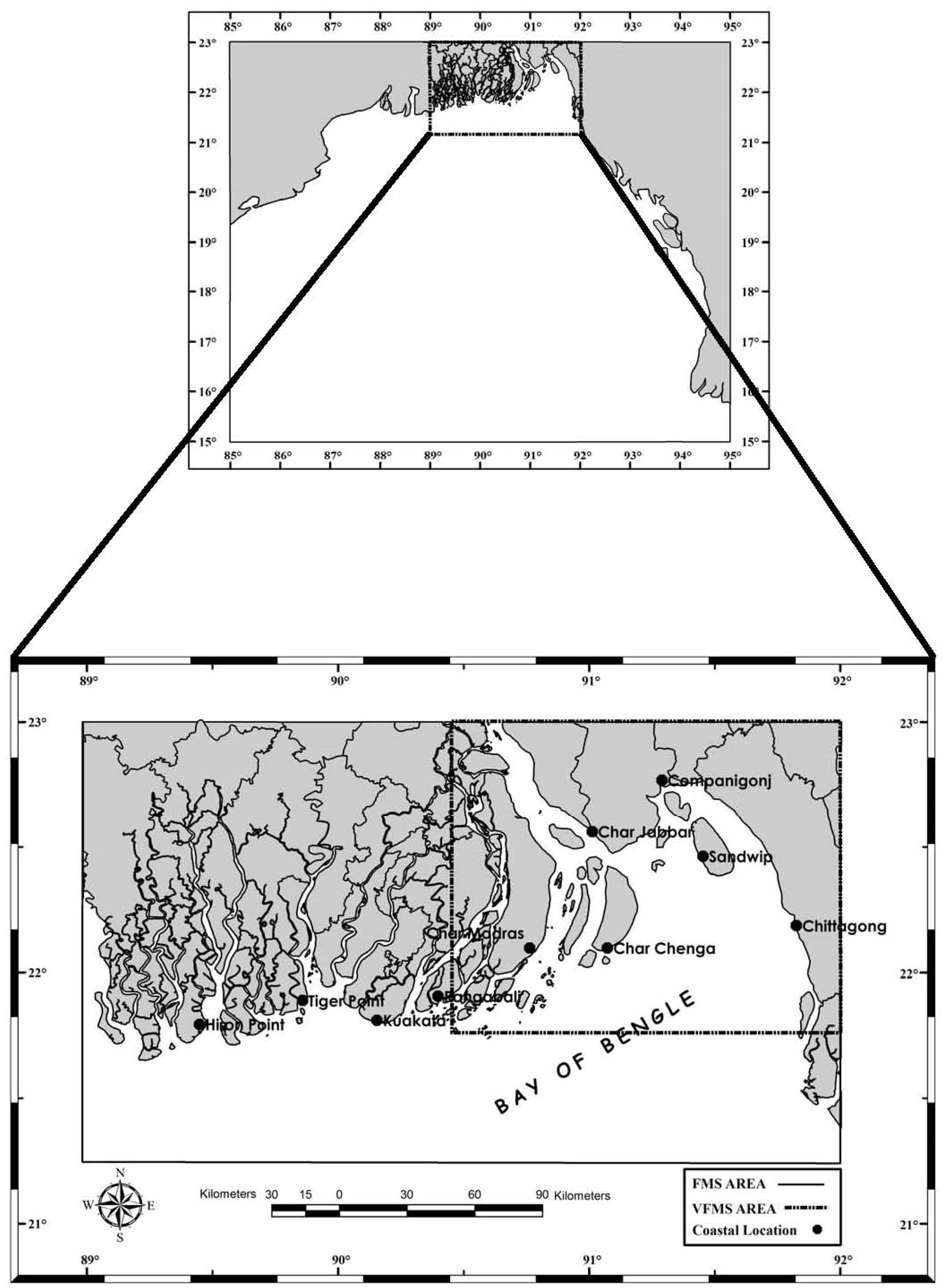
Figure 1. Domains of the three schemes CMS, FMS and VFMS and actual coastal and island boundaries along with ten representative locations at which computed results are presented (after Paul et al. [9]).
Environsciproc 05 00007 g001
Figure 2. Computed water levels with respect to the mean sea level due to tide, surge and their interaction with observed data at Hiron Point, Char Chenga and Chittagong. In each subplot, a black dotted curve represents the configuration for tide, black solid curve for surge, red dotted curve for tide–surge interaction, and a circle represents observed data.
Environsciproc 05 00007 g002
Table 1. Time series for the positions and the nature of the April 1991 cyclone (Source: BMD).
Date (1991)Hour (UTC)Latitude (°N)Longitude(°E)Nature of the Storm
26 April180011.8087.50Cyclonic storm
27 April030012.5087.50Cyclonic storm
27 April060013.0087.50Cyclonic storm
27 April090013.6087.50Severe cyclonic storm
27 April180014.5087.50Severe cyclonic storm with hurricane core
28 April060015.8087.70Severe cyclonic storm with hurricane core
28 April080016.5088.00Severe cyclonic storm with hurricane core
28 April180017.6088.30Severe cyclonic storm with hurricane core
29 April060019.8089.40Severe cyclonic storm with hurricane core
29 April120020.8090.40Severe cyclonic storm with hurricane core
29 April180022.0091.40Severe cyclonic storm with hurricane core
29 April200022.3091.80Crossing the coast near Chittagong
30 April000023.0092.40Crossed the Bangladesh coast
30 April020023.5092.80--
Maximum wind speed: 234 km h−1, maximum radius of sustained wind: 50 km.
Table 2. Domains, grid resolutions and number of grid points of different schemes (after Paul et al. [9]).
ModelDomain ExtentGrid Resolution Along x-AxisGrid Resolution Along y-AxisNumber of Grid Points
CMS 15 23 N and 85 95 E15.08 km17.52 km60 × 61
FMS 21.25 and 89 92 E2.15 km3.29 km92 × 95
VFMS 21.77 23 N and 90.40 92 E 720.73 m1142.39 m190 × 145
Table 3. Computed peak water levels simulated by the present study with respect to the mean sea level (MSL) and those obtained in [6].
Coastal LocationPresent StudyStudy due to Paul et al. [6]
Simulated Maximum Surge Level (m)Simulated Maximum Total Water Level (m)Maximum Surge Level (m)Maximum Total Water Level (m)
Hiron point2.973.323.924.01
Tiger point4.114.514.214.57
Kuakata3.253.823.523.86
Char Chenga5.705.895.115.81
Char Jobbar6.126.336.196.35
Companigonj6.516.306.707.28
Sandwip5.405.715.245.63
Chittagong5.295.795.176.26
Table 4. Estimated RMSEs in meters. The errors have been estimated between computed and observed water levels from 02.00 UTC of April 28 to 02.00 UTC of April 30 for the storm in April 1991. The observed data were obtained from BIWTA.
Costal StationEstimated by the ModelEstimated by the Model Due to Paul et al. [9]
Chittagong0.780.73
Char Chenga0.550.58
Hiron Point0.180.16
Publisher’s Note: MDPI stays neutral with regard to jurisdictional claims in published maps and institutional affiliations.