Next Article in Journal
Estimation of Crop Production and CO2 Fluxes Using Remote Sensing: Application to a Winter Wheat/Sunflower Rotation
Previous Article in Journal
Testing the Drop-Size Distribution Based Separation of Stratiform and Convective Rain Using Radar and Disdrometer Data from a Midlatitude Coastal Region
 
 
Please note that, as of 4 December 2024, Environmental Sciences Proceedings has been renamed to Environmental and Earth Sciences Proceedings and is now published here.
Proceeding Paper

Investigation of Precipitation Variability and Extremes Using Information Theory †

Department of Hydrology, Indian Institute of Technology Roorkee, Uttarakhand 247667, India
*
Author to whom correspondence should be addressed.
Presented at the 3rd International Electronic Conference on Atmospheric Sciences, 16–30 November 2020; Available online: https://ecas2020.sciforum.net/.
Environ. Sci. Proc. 2021, 4(1), 14; https://doi.org/10.3390/ecas2020-08115
Published: 13 November 2020
(This article belongs to the Proceedings of The 3rd International Electronic Conference on Atmospheric Sciences)

Abstract

:
Quantifying the spatiotemporal variability of rainfall is the principal component for the assessment of the impact of climate change on the hydrological cycle. A better understanding of the quantification of variability and its trend is vital for water resources planning and management. Therefore, a multitude of studies has been dedicated to quantifying the rainfall variability over the years. Despite their importance for modelling rainfall variability, the studies mainly focused on the amount of rainfall and its spatial patterns. The studies investigating the spatial and temporal variability of rainfall across Central India, in general, and at multiscale, in particular, are limited. In this study, we used a Standardized Variability Index (SVI), based on information theory to investigate the spatiotemporal variability of rainfall. SVI is independent of the temporal scale, length of the data and can compare the rainfall variability at multiple timescales. Distinct spatial patterns were observed for information entropies at the monthly and seasonal scale. Grid points with statistically significant trends were observed and vary from monthly to seasonal scale. There is an increase in the variability of rainfall amount from South to North, indicating that spread of the rainfall is high in the South when compared to North of Central India. Trend analysis revealed there is changing behavior in the rainfall amount as well as rainy days, showing an increase in variability of rainfall over Central India, hence the high probability of occurrence of extreme events in the near future.

1. Introduction

Rainfall is a reliable feature for the Indian subcontinent and highly uncertain in space and time. Rain is the primary component of the hydrological cycle, describes the transfer of energy between earth and atmosphere. In the cyclic process of atmospheric circulation, there is a high impact of global warming-induced climate change on the components of the hydrological cycle and its variability [1]. As a consequence, there is a significant variation in the average rainfall, temperature, evaporation and change of rate, timing and distribution of rainfall [2]. The spatiotemporal variability of rainfall has a significant impact on agricultural productivity, and the Indian economy depends on the monsoon rains and accounts for 22% of Indian gross domestic product.
In the past decade, several types of research conducted on spatiotemporal variability of Indian rainfall out of these, Chandniha et al., conducted trend analysis of mean rainfall for Jharkhand State using monthly rainfall time series for 111 years (1901–2011) using data from 18 meteorological stations [3]. They concluded that mean rainfall is increasing for the first half of the century (1901–1949) and later part of the century is characterized (1950–2011) with a decreasing trend. Das et al., conducted a spatial analysis of temporal trend analysis of rainfall during Indian summer monsoon using 0.5° × 0.5° daily gridded data for a period starting from 1975 to 2005 [4]. An increasing trend of rainfall is observed in the east coast, Deccan plateau and northern hilly parts of the Himalaya. The decreasing trend of rainfall is observed in the west coast, western arid region, eastern plain and northeastern humid region. The increasing trend of rainy days is observed for the east coast, Deccan plateau and decreasing trend for the west coast, western arid region, northern hilly parts of the Himalaya, north and central plains. An investigation on spatiotemporal variability of rainfall for 45 districts in Madhya Pradesh by Duhan and Pandey over 102 years (1901–2002), detected 1978 as the most probable year for change in annual rainfall [5]. On comparing the percentage of change in the mean annual rainfall of 1901–1978 relative to 1979–2002, there is a decrease in the rainfall in all stations after 1978. Guhathakurta and Rajeevan conducted the trend of rainfall pattern over India for 36 meteorological subdivisions during the south-west monsoon [6]. It is found that Gangetic West Bengal, West Uttar Pradesh, Jammu and Kashmir, Konkan and Goa, Madhya Maharashtra, Rayalseema, Coastal Andhra Pradesh and North Interior Karnataka showed significant increasing trends and Jharkhand, Chattisgarh, Kerala showed a decreasing trend.
Kumar et al., studied monthly, seasonal and annual trends of rainfall using monthly data series of 135 years (1871–2005) for 30 sub-divisions (sub-regions) in India [7]. Haryana, Punjab and Coastal Karnataka showed a statically significant increasing trend in annual rainfall. Chattisgarh subdivision showed a decreasing trend in annual rainfall. Spatiotemporal variability of rainfall for Chattisgarh State by Meshram et al., exhibited a decreasing trend at all stations except Bilaspur and Dantewada [8]. Rajeevan et al., examined the variability and long-term trends over central India [9]. There exists a coherent relationship between the sea surface temperature and rainfall extremes and suggest an increase in the risk of significant floods over central India. Sanikhani et al., evaluated rainfall trend of Central India for monthly, seasonal, and annual time scales using monthly rainfall data and concluded there is no significant trend in the stations for the January and October months [10]. The results also showed that for Chattisgarh, four out of five considered stations does not indicate a significant annual trend, while in Madhya Pradesh, two out of fifteen stations exhibited a significant trend. Variability is defined as the lack of uniformity over different class intervals [11]. Very recently, Guntu et al., proposed Standardized Variability Index (SVI) to quantify the inter-annual and intra-annual variability and found to be robust than traditional approaches [12].
There are minimal studies on the spatiotemporal variability of rainfall over Central India using 0.25° × 0.25° daily rainfall gridded data, in particular at multiple time scales. Still, a research gap exists in categorizing the grid points with abundant water resources. Categorization of most probable water resources helps in identifying the potential regions, and it is essential for water resources planning and management [11]. In this paper attempt is made to address the following objectives:
  • To investigate the inter-annual variability of rainfall on a monthly, seasonal and annual time scale and intra-annual variability at monthly time scale using SVI
  • To develop a correlation between the intra-annual variability (SVI) and mean annual rainfall, thereby to classify the grid points with promising water resources availability.

2. Study Area and Data

In this study, we use the gridded data of daily average rainfall (mm) developed by Pai et al., with a high spatial resolution of 0.25° × 0.25° covering the Central India [73.50° E–83.50° E and 18° N–25° N] [13]. The daily data for a period of 119 years (1901–2019) is obtained from the archive of the National Data Centre, IMD, Pune.
In the present study, the four seasons are defined in terms of months as follows: March–April–May (MAM), which is the summer season; June–July–August (JJA), which is the southwest monsoon season; September–October–November (SON), which is the autumn (or fall) season, during which much of the northeast monsoon also occurs; and December–January–February (DJF), which is the winter season. For the inter-annual variability, we consider the monthly, seasonal, and annual timescales; and for the intra-annual variability at the monthly timescale following Guntu et al. [12]. This detailed investigation of the rainfall pattern would provide a comprehensive picture of the spatiotemporal rainfall variability. The geographical location and spatiotemporal variability of rainfall of the study area are presented in the Figure 1.

3. Methodology

3.1. Entropy-Based Metrics

Shannon entropy concept of measure of information/uncertainty is used in this study to determine the disorder of the rainfall variability in terms of space and time. Singh discussed entropy theory applications in environmental and water engineering which includes rainfall-runoff modeling, infiltration, soil moisture, groundwater flow, river hydraulics [14]. The advantages and limitations of entropy derived metrics are briefly described in [15].
The generalized equation defining entropy (H), is defined as [16].
H ( X ) = i = 1 N P ( x i ) l o g 2 [ p ( x i ) ]
where P : { P 1 , P 2 , . . P N } is the probability distribution of X, N is the sample size. l o g 2 P ( x i ) is the measure of uncertainty about the event occurring with probably P ( x i ) . H ( X ) is the entropy of P : { P 1 , P 2 , . . P N } , and H ( X ) is expressed in terms of bits [11], For a deterministic variable, if the entropy H ( X ) is zero then it has minimum uncertainty/Maximum certainty, about the probability that it will take on a particular value is 1, and the probabilities of all other alternative values are zero. On the other side if all the events are equally likely, then the distribution is highly uncertain, and it is equal to l o g 2 N .

3.2. Marginal Entropy (ME)

The variability of a rainfall time series spatially and temporally can be quantitatively measured by using entropy. The marginal entropy H ( X ) measures the degree of uncertainty about the random variable X with the probability distribution P ( X ) . It is calculated from a single historical time series and it gives disorder contained within the entire length of time scale. In the present study, to understand the spatial distribution of disorder based on the amount of rainfall over the 119 years, rainfall time series of different time scales (annual, seasonal, monthly) were considered [2]. The mathematical expression of ME is given by Equation (1).

3.3. Apportionment Entropy (AE)

To study the variability of the amount of rainfall of months within year Apportionment entropy is used [17]. Considering the amount of rain ( r i ) in a month, (i = 1, 2, 3, …, 12) of a year to the total amount of rain in that year (R), the likeliness will be r i R , denoted by P i . Probabilities for a particular grid point are expressed in discrete form by taking into account all the aggregate rainfall available at that grid point and their likeliness. Finally, using Shannon entropy, AE can be calculated from Equation (2).
A E ( X ) = i = 1 R P ( x i ) l o g 2 [ p ( x i ) ]
where P ( x i ) = r i R ; R is the number of class intervals. Maximum AE is the l o g 2 12 when the variability of the amount of rainfall of months within a year is extremely low.

3.4. Standardized Variability Index (SVI)

In this study, we employed the Standardized variability index (SVI) proposed by Guntu et al., to quantify the variability and defined as Equation (3) [12]
S V I = H m a x H H m a x
where Hmax is the maximum entropy that can be obtained for a given distribution and H is the entropy obtained for the given time series. SVI is a single outcome which can represent the number of events majorly contributed to the formation of the random variable, and it defines the variability associated with discrete-time series regarding maximum possible variability. From the description, SVI takes on a value within a finite range of 0 to 1, where zero matches to no variability and one represent high variability, i.e., minimum uncertainty to maximum uncertainty. As the SVI increases, variability increases and vice versa. Since the range of SVI is finite and it has a competence of inter-comparison of results for datasets with different length of the data and at multiple time scales.

4. Results

4.1. Inter-Annual Variability

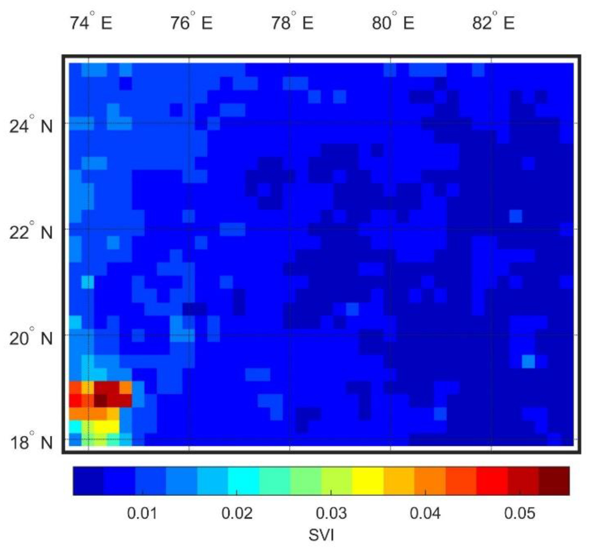
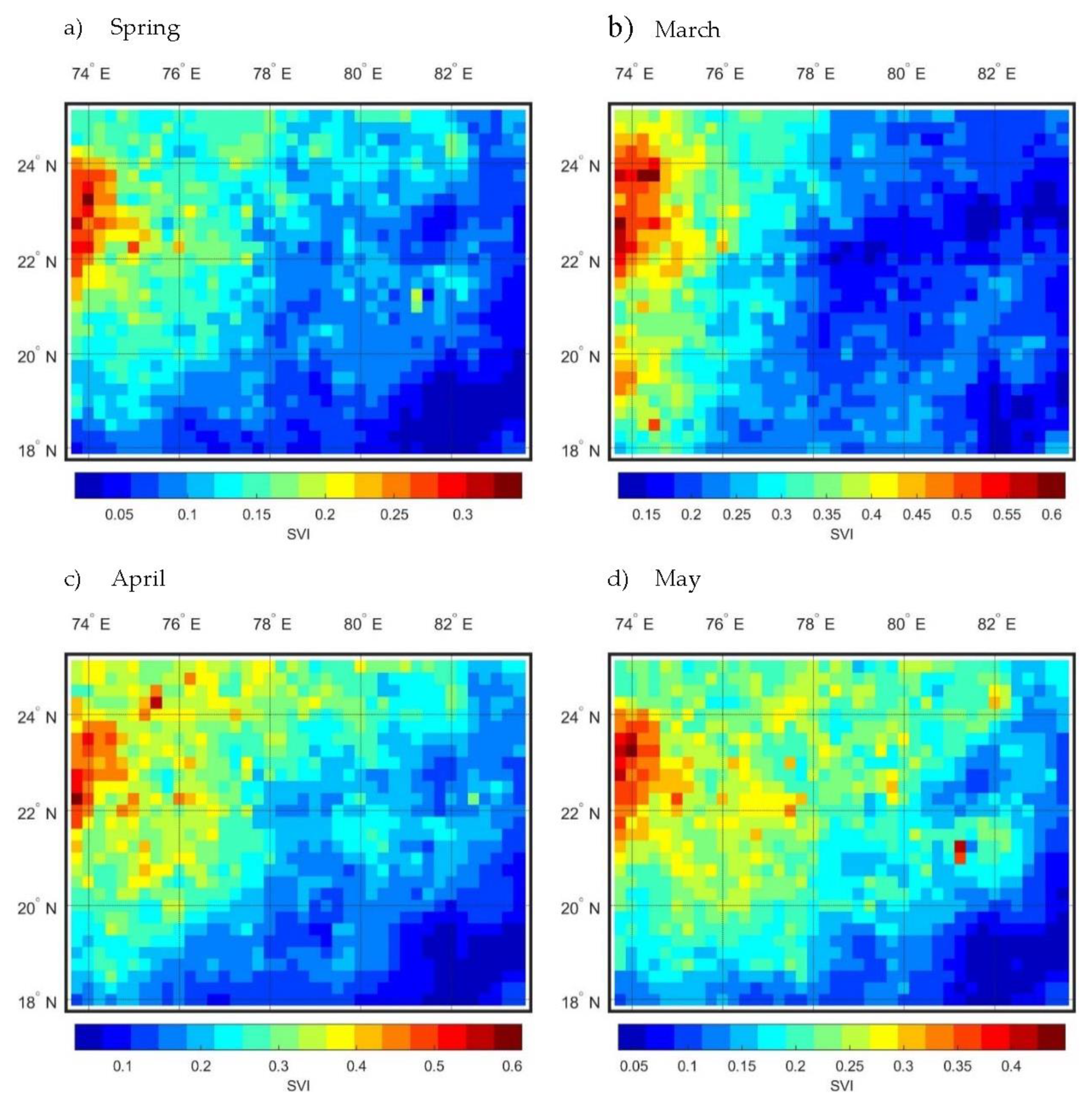
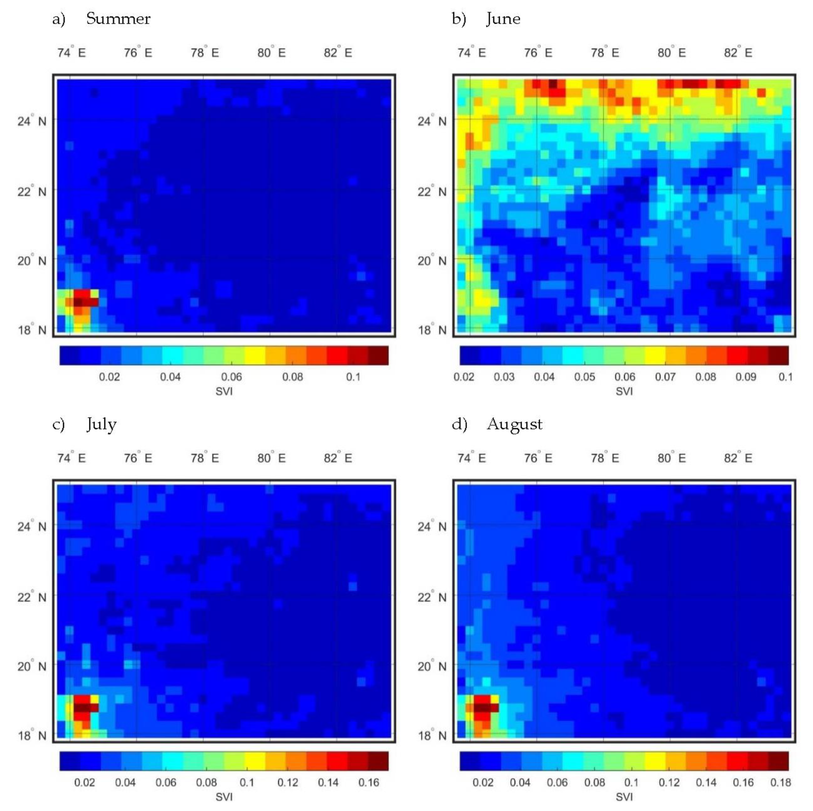
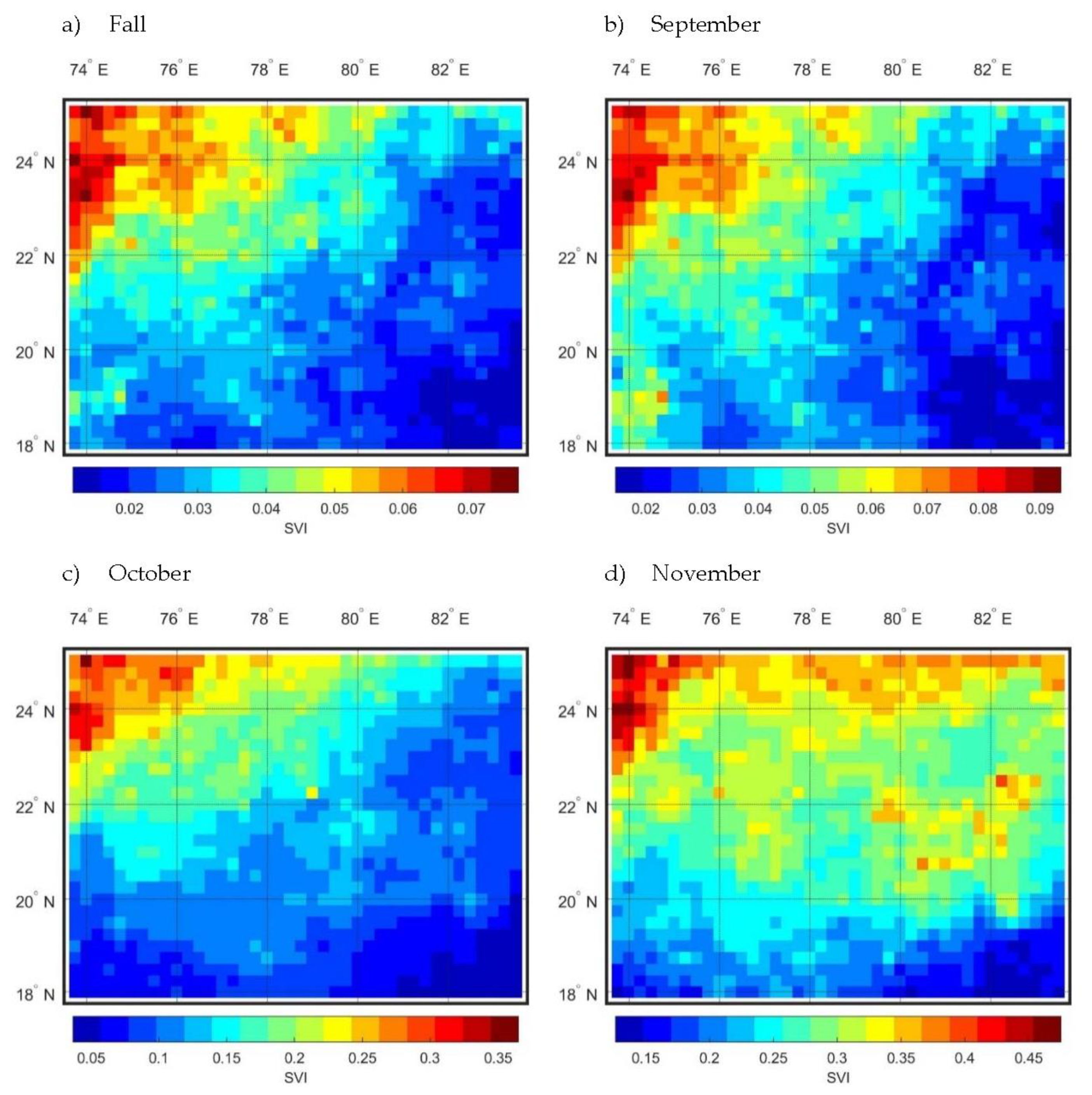
To investigate the interannual variability, the daily rainfall data is converted into annual, seasonal and monthly rainfall time-series. The ME is calculated based on the rainfall amount considered for the respective time series for every grid point. The annual rainfall variability is more for the points corresponding to the South-west region (see Figure 2). The ME of annual time series is more than the seasonal time series, i.e., the variability of annual rainfall is less than the seasonal rainfall. Spatial variability of ME representing the seasons and its constituent months are plotted in Figure 3, Figure 4, Figure 5 and Figure 6.
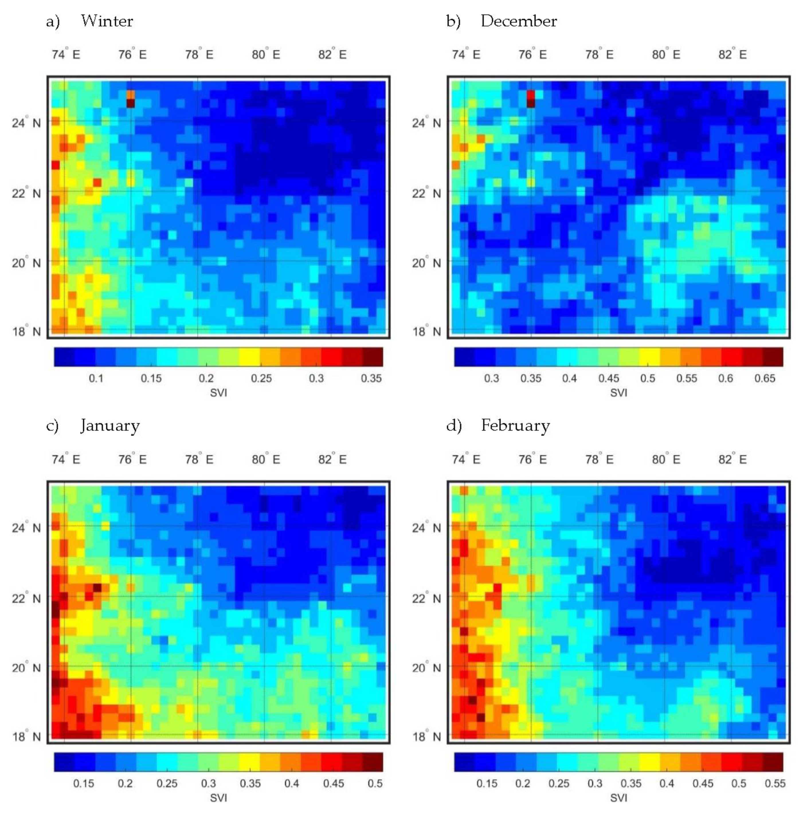
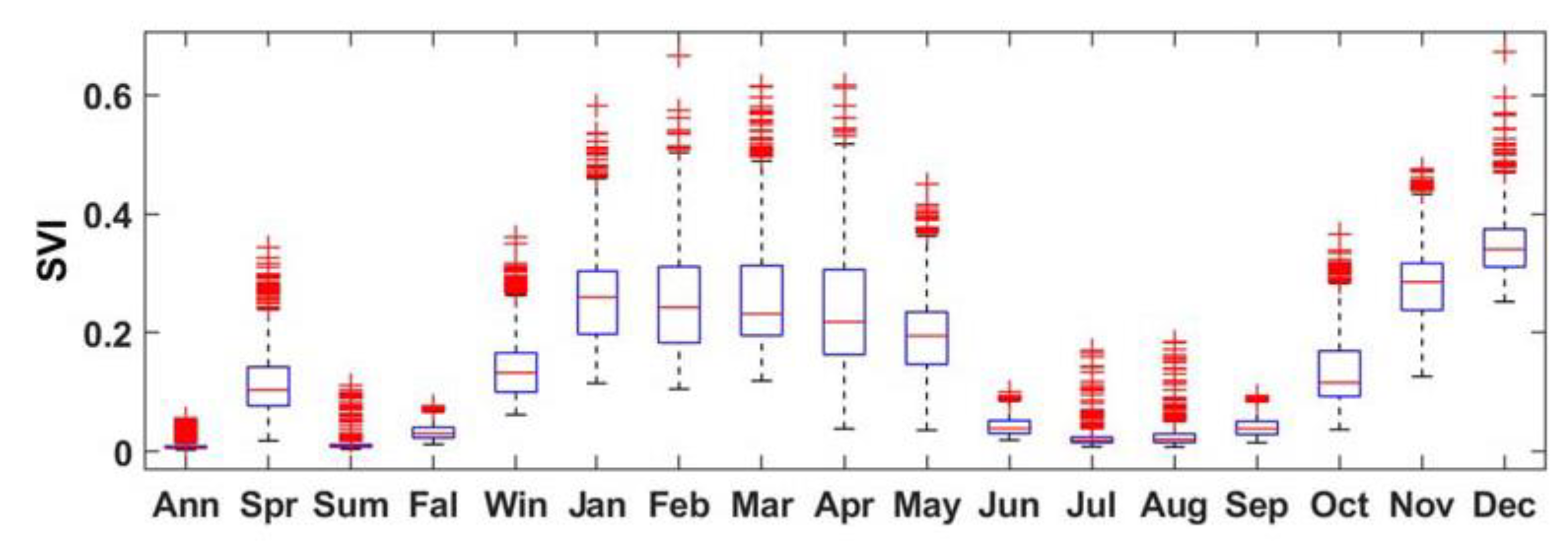
Spring rainfall has low variability in the western region of Central India (see Figure 3a). Summer rainfall has low variability all over the study area due to the Indian Summer Monsoon (ISM) (see Figure 4), fall rainfall is more variable in the regions of the northwest of the study area (see Figure 5), winter rainfall has high variability in the west region of the study area (see Figure 6). To understand the months responsible for the seasonal variability, the inter-variability of months within the season should be analyzed. The SVI of seasonal time series is more than the monthly time series, i.e., the variability of seasonal rainfall is less than the monthly rainfall. Box plot of SVI corresponding to annual, seasons and months are shown in Figure 7. Summer contributed less to the annual variability and winter contribution is the highest. In the variability of the spring season and its constituent months, May contributed low to the rainfall variability and March contribution is the highest. In the summer season and its constituent months, June contributed less to the rainfall variability and august contribution is the highest. In the fall season, September contributed less to the rainfall variability and November contribution is the highest. In winter season December contributed less to the rainfall variability and January contribution is the highest. Overall, the spatial pattern of SVI at the monthly time scale reflects the consistency in the seasonality of rainfall over the years. For instance, the southwest monsoon has low variability across the Southeast of Central India during June. In July and August, the spatial pattern of low variability is moving towards the North-west of Central India. The spatial pattern of SVI in September discloses the presence of southwest monsoon and the onset of the northeast monsoon (the southeastern region of Central India). The northeast monsoon is shifting from northwest to the south of Central India in October, November and December. Further, northeastern monsoon plays a significant role in the south of the basin during the fall season. In January to May, the spatial pattern of SVI reveals high interannual variability over west of Central India. The unseasonal rains received during these months is due to the tropical cyclonic activities, has high uncertainty.

4.2. Intra-Annual Variability

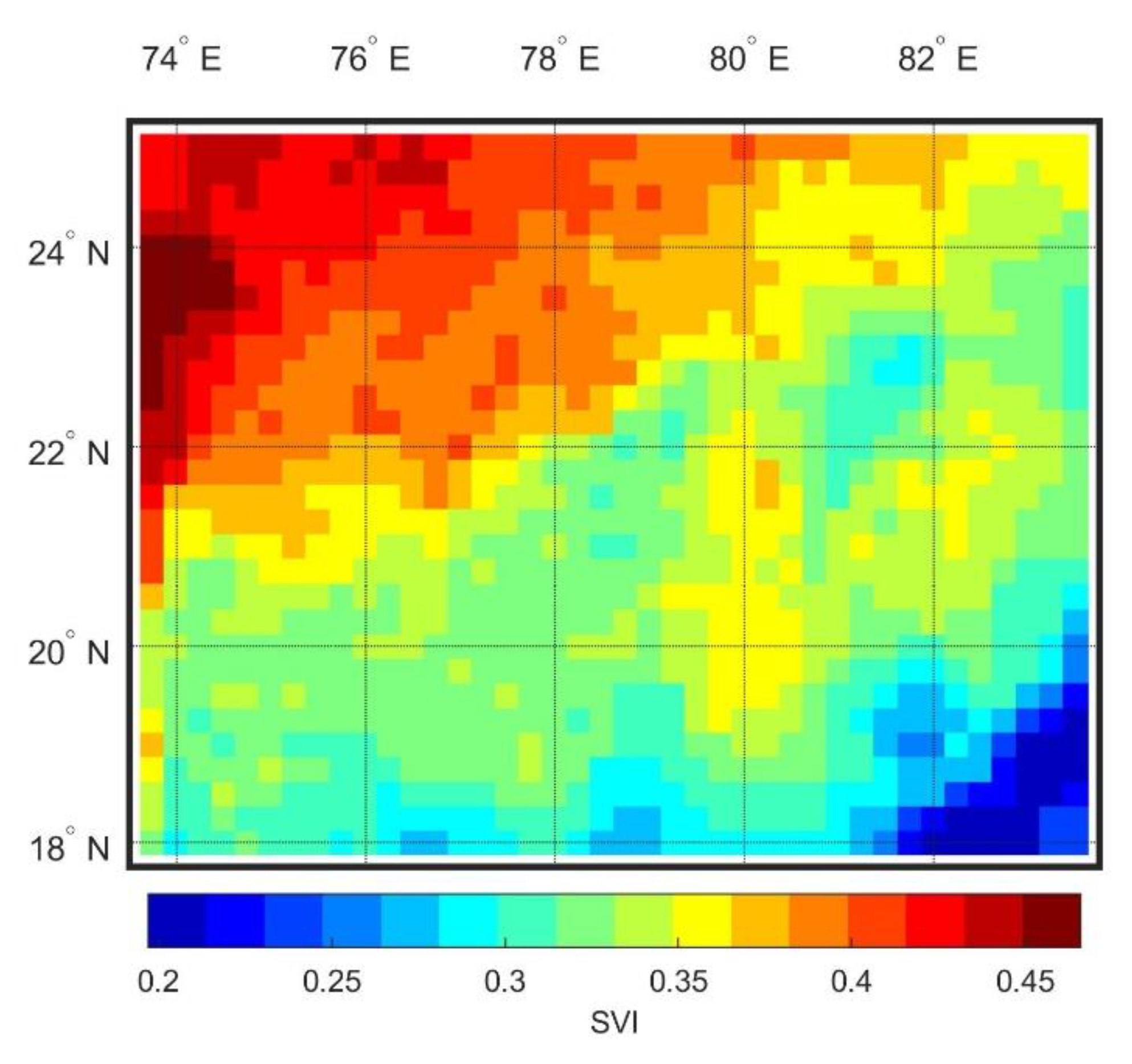
After summarizing the interannual variability of annual, seasonal and monthly rainfall time series, it is crucial to examine the rainfall distribution within the year, and it is essential to highlight the grid points corresponding to high variability. Apportionment entropy is applied to investigate the monthly variation of rainfall within the year based on the rainfall. From the obtained AE, 119 SVI values from 1901–2019 are calculated for every grid point. Further, average SVI from 119 values is calculated for every grid point and is represented in Figure 8. From the map, it shows that the variability is decreasing from northwest to southeast. In particular, the variability is more in the northwest region, and it tells us that the rainfall is concerned to only a few months in a year in those regions. In the southeast region of the study area variability is low, indicating widespread rainfall distribution.

5. Discussion

The mean annual rainfall and variability within the year help to classify the grid points with abundant water resources. Therefore, the coupling of mean annual rainfall with average SVI results in identifying the grids having a fair amount of rain with perennial supply. Figure 9a represents the scattered plot of SVI on the ordinate and mean annual rainfall on the abscissa. The 50th percentile of mean annual rainfall and SVI is calculated and plotted as lines, and these helped to delineate the total scattered plot into four classes, A, B, C, D and the classes are classified as follows:
Class-A receives a high amount of rainfall with low variability, and it gives us the information that water resources are abundant and perennially available at that grids. This class of people can use water resources willfully being only subjected to the permissible water withdrawal from the natural water cycle.
Class-B. Receive a low amount of rainfall with low variability, and it gives us the information that water resources are moderate and perennially available at that grids. Water resources development and management are required to raise availability during the spells of high water demand.
Class-C. Receive a low amount of rainfall with high variability, and it gives us the information that water resources are insufficient and not perennial. To meet the yearly water demand, there is a need to increase disposable water resources by the construction of water storage facilities.
Class-D. Receive a high amount of rainfall with high variability high, and it gives us the information that grids are concentrated with heavy rain and water control is needed for the flood management in parallel with the storage of surplus water in the reservoirs.
The grids corresponding to each class developed from the coupling of SVI and rainfall are plotted as the same color in Figure 9b. From the figure, we can see that majority of the grid points falling under Class-C and D lies in the north region of the study area.
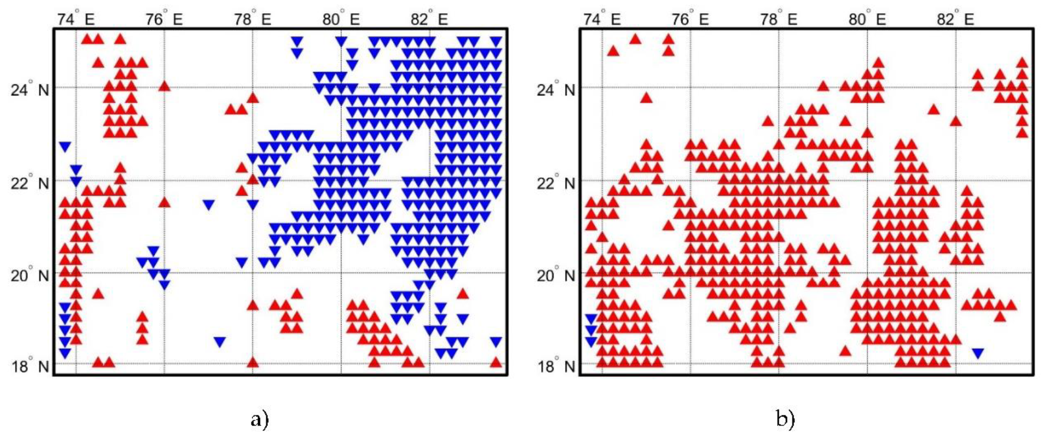
To understand the temporal pattern of mean annual rainfall and SVI non-parametric Mann-Kendall trend test is applied [18,19]. We conducted a trend analysis of mean annual rainfall and SVI for every grid point with a 95% confidence limit. The spatial representation of grid points with a significant trend is shown in Figure 10. The increasing trend represents an increase in rainfall variability over the years, which in turn indicates that rainfall gets more concentrated only during a certain period of the year. On the other hand, a decreasing trend suggests that the spread of rain within a year increases. Therefore, the north region has high intra-annual variability and face extreme events in the near future in the form of droughts and floods.

6. Conclusions

We have applied the entropy-based analysis to investigate the inter-annual and intra-annual variability at multiple time scales. Finally, coupling of SVI and mean annual rainfall helps in identifying the grids with potential water resources with perennial supply and to extremes. From the analysis, the following conclusions are drawn.
  • The inter-annual variability of rainfall for annual time series is less than the seasonal time series, summer contributed least and winter highest to the annual variability. Spatial variability of the seasons and months show distinct patterns indicating an inconsistency in the rainfall pattern.
  • The intra-annual variability based on the amount of rainfall considering at monthly time scale shows that the variability is increasing from southeast to northwest of Central India.
  • Coupling of the SVI with the mean annual rainfall as a correlation measure found north half with high variability and south half with low variability in terms of rainfall amount.

Author Contributions

Conceptualization, R.K.G. and A.A.; methodology, R.K.G. and A.A.; software, R.K.G.; formal analysis, R.K.G.; writing—original draft preparation, R.K.G.; writing—review and editing, A.A. All authors have read and agreed to the published version of the manuscript.

Funding

RKG was supported by the Inspire fellowship award under DST, India under grant No. IF 190581. AA acknowledge the joint funding support from the University Grant Commission (UGC) and DAAD under the framework of the Indo-German Partnership in Higher Education (IGP).

Institutional Review Board Statement

Not applicable.

Informed Consent Statement

Not applicable.

Data Availability Statement

Not applicable.

Conflicts of Interest

The authors declare no conflict of interest.

References

  1. Guntu, R.K.; Maheswaran, R.; Agarwal, A.; Singh, V.P. Accounting for temporal variability for improved precipitation regionalization based on self-organizing map coupled with information theory. J. Hydrol. 2020, 590, 125236. [Google Scholar] [CrossRef]
  2. Mishra, A.K.; Özger, M.; Singh, V.P. An entropy-based investigation into the variability of precipitation. J. Hydrol. 2009, 370, 139–154. [Google Scholar] [CrossRef]
  3. Chandniha, S.K.; Meshram, S.G.; Adamowski, J.F.; Meshram, C. Trend analysis of precipitation in Jharkhand State, India. Theor. Appl. Clim. 2016, 130, 261–274. [Google Scholar] [CrossRef]
  4. Das, P.K.; Chakraborty, A.; Seshasai, M.V.R. Spatial analysis of temporal trend of rainfall and rainy days during the Indian Summer Monsoon season using daily gridded (0.5° × 0.5°) rainfall data for the period of 1971–2005. Meteorol. Appl. 2014, 21, 481–493. [Google Scholar] [CrossRef]
  5. Duhan, D.; Pandey, A. Statistical analysis of long term spatial and temporal trends of precipitation during 1901–2002 at Madhya Pradesh, India. Atmospheric Res. 2013, 122, 136–149. [Google Scholar] [CrossRef]
  6. Guhathakurta, P.; Rajeevan, M. Trends in the rainfall pattern over India. Int. J. Clim. 2008, 28, 1453–1469. [Google Scholar] [CrossRef]
  7. Kumar, V.; Jain, S.K.; Singh, Y. Analysis of long-term rainfall trends in India. Hydrol. Sci. J. 2010, 55, 484–496. [Google Scholar] [CrossRef]
  8. Meshram, S.G.; Singh, V.P.; Meshram, C. Long-term trend and variability of precipitation in Chhattisgarh State, India. Theor. Appl. Clim. 2017, 129, 729–744. [Google Scholar] [CrossRef]
  9. Rajeevan, M.; Bhate, J.; Jaswal, A.K. Analysis of variability and trends of extreme rainfall events over India using 104 years of gridded daily rainfall data. Geophys. Res. Lett. 2008, 35. [Google Scholar] [CrossRef]
  10. Sanikhani, H.; Kisi, O.; Mirabbasi, R.; Meshram, S.G. Trend analysis of rainfall pattern over the Central India during 1901–2010. Arab. J. Geosci. 2018, 11, 437. [Google Scholar] [CrossRef]
  11. Kawachi, T.; Maruyama, T.; Singh, V.P. Rainfall entropy for delineation of water resources zones in Japan. J. Hydrol. 2001, 246, 36–44. [Google Scholar] [CrossRef]
  12. Guntu, R.K.; Rathinasamy, M.; Agarwal, A.; Sivakumar, B. Spatiotemporal variability of Indian rainfall using multiscale entropy. J. Hydrol. 2020, 587, 124916. [Google Scholar] [CrossRef]
  13. Pai, D.S.; Sridhar, L.; Rajeevan, M.; Sreejith, O.P.; Satbhai, N.S.; Mukhopadhyay, B. Development of a new high spatial resolution (0.25° × 0.25°) long period (1901–2010) daily gridded rainfall data set over India and its comparison with existing data sets over the region. Mausam 2014, 65, 1–18. [Google Scholar] [CrossRef]
  14. Singh, V.P. Hydrologic Synthesis Using Entropy Theory: Review. J. Hydrol. Eng. 2011, 16, 421–433. [Google Scholar] [CrossRef]
  15. Singh, V.P. The Use of Entropy in Hydrology and Water Resources. Hydrol. Process. 1997, 11, 587–626. [Google Scholar] [CrossRef]
  16. Shannon, C.E. A Mathematical Theory of Communication. Bell Syst. Tech. J. 1948, 27, 379–423. [Google Scholar] [CrossRef]
  17. Maruyama, T.; Kawachi, T.; Singh, V.P. Entropy-based assessment and clustering of potential water resources availability. J. Hydrol. 2005, 309, 104–113. [Google Scholar] [CrossRef]
  18. Mann, H.B. Nonparametric tests against trend. Econometrica 1945, 13, 245–259. [Google Scholar] [CrossRef]
  19. Kendall, M.G. Rank Correlation Measures; Charles Griffin: London, UK, 1975. [Google Scholar]
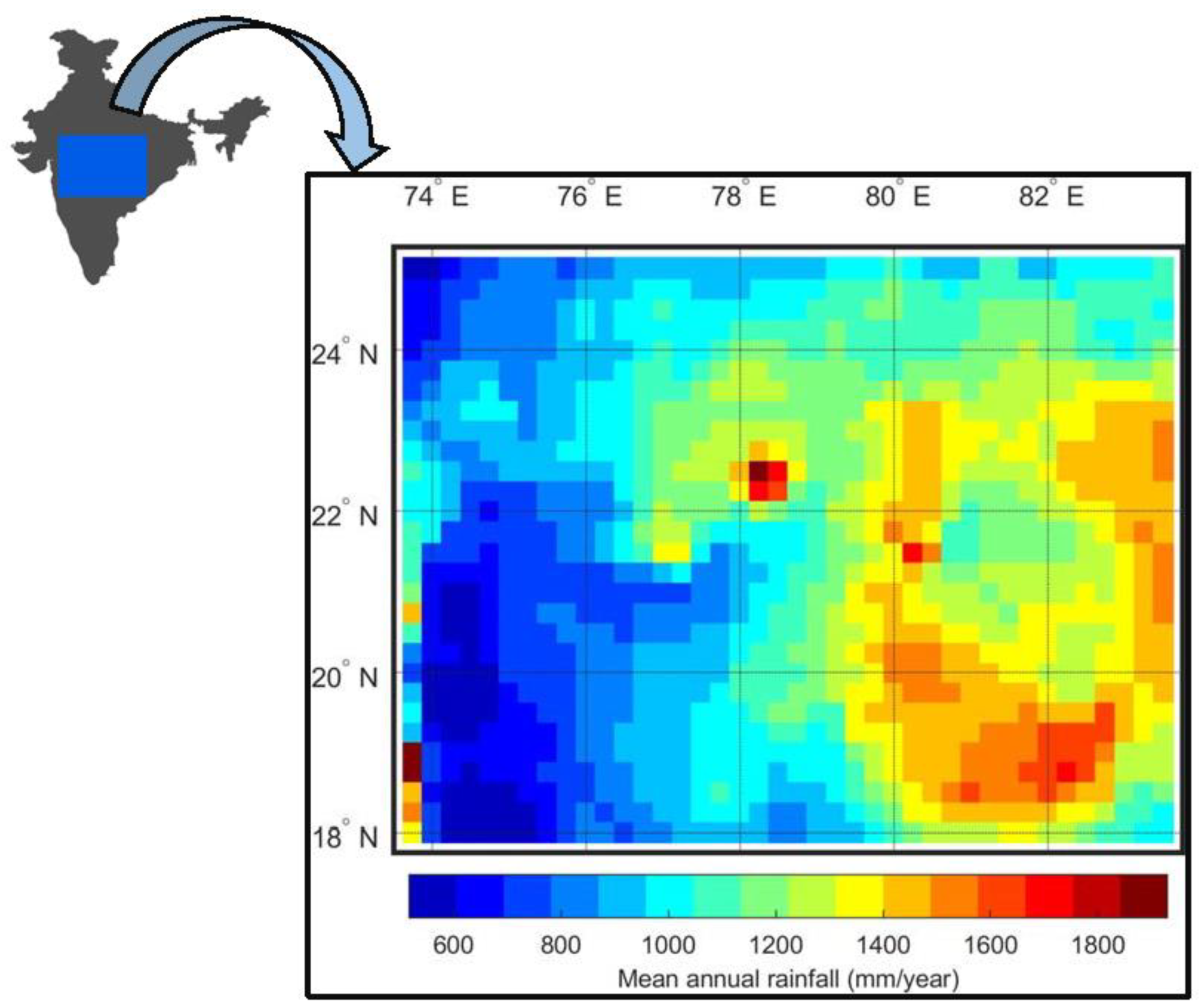
Figure 1. Spatiotemporal pattern of the mean annual rainfall over Central India during 1901–2019.
Environsciproc 04 00014 g001
Figure 2. Spatial distribution of interannual variability of annual rainfall over the period from 1901–2019.
Environsciproc 04 00014 g002
Figure 3. Spatial distribution of inter-annual variability of (a) Springtime series and its constituent months (March (b), April (c) and May (d)).
Environsciproc 04 00014 g003
Figure 4. Spatial distribution of inter-annual variability of (a) Summertime series and its constituent months (June (b), July (c) and August (d)).
Environsciproc 04 00014 g004
Figure 5. Spatial distribution of inter-annual variability of (a) Fall time series and its constituent months (September (b), October (c) and November (d)).
Environsciproc 04 00014 g005
Figure 6. Spatial distribution of inter-annual variability of (a) Wintertime series and its constituent months (December (b), January (c) and February (d)).
Environsciproc 04 00014 g006
Figure 7. Box plot of SVI corresponding to annual, seasonal and monthly time scale.
Environsciproc 04 00014 g007
Figure 8. Spatial distribution of intra-annual variability of monthly rainfall time series.
Environsciproc 04 00014 g008
Figure 9. (a) Plot between mean annual rainfall and its variability (in terms of SVI) and (b) Geographical locations of the grid points falling under different classes.
Environsciproc 04 00014 g009
Figure 10. Spatial pattern of the trend of (a) Rainfall and (b) SVI based on Mann-Kendall trend test. Upward triangles (red) indicates an increasing trend and downward triangles (blue) indicates decreasing trend.
Environsciproc 04 00014 g010
Publisher’s Note: MDPI stays neutral with regard to jurisdictional claims in published maps and institutional affiliations.