Proceeding Paper

Impact of Land Use and Land Cover Changes on the Stream Flow and Water Quality of Big Creek Lake Watershed South Alabama, USA †

1
Department of Geography, The Ohio State University, Columbus, OH 43210, USA
2
Department of Geosciences, Auburn University, Auburn, AL 36849, USA
*
Author to whom correspondence should be addressed.
Presented at the ICSD 2021: 9th International Conference on Sustainable Development, Virtual, 20–21 September 2021.
Environ. Sci. Proc. 2022, 15(1), 9; https://doi.org/10.3390/environsciproc2022015009
Published: 1 April 2022
(This article belongs to the Proceedings of The 9th International Conference on Sustainable Development)

Abstract

:
Land use is one of the key factors affecting the stream flow of a watershed. This research aimed to evaluate the impact of changing land use and land cover (LULC) on stream flow and water quality by applying the Soil and Water Assessment Tool (SWAT) to the Big Creek Lake watershed located in Mobile County, South Alabama. Digital elevation model (DEM), LULC data, weather data, soil data, observed streamflow, nitrogen, and phosphors data were used as input files to calibrate and validate the SWAT model. The SWAT model was calibrated and validated using the Sequential Uncertainty Fitting (SUFI-2) algorithm in the SWAT Calibration Uncertainties Program (SWAT-CUP) software. Agricultural land increased by about 11,045 acres and urban area increased by 3350 acres, and forest area decreased by 11,482 acres, between 1991 and 2020. This changing scenario of LULC not only increased the streamflow but also the total nitrogen and phosphorus. The total streamflow was higher, at about 38 m3/s in the LU_2020 scenario, than in the LU_1990 scenario. Increases of about 1,136,919 kg of nitrogen and 324,467 kg of phosphorus were found from 1990 to 2020, and these increases can be explained by an increase in agricultural land of about 11,045 acres. The results obtained in this study are able to provide guidance to water resource management and planning for policymakers and water managers in Mobile County.
Keywords:
LULC; DEM; SWAT; SUFI-2

1. Introduction

According to [1,2,3] in recent decades, hydrological responses to the changing environment have become a research interest area. Changing land use and land cover (LULC) influence runoff–rainfall processes by affecting the surface components such as evapotranspiration, infiltration, and percolation. Various types of land use have different reflectivity (albedo), roughness, leaf areas, and soil depth, which impacts the land–surface interactions by affecting temperature, humidity, wind speed, and precipitation [4,5,6]. Changes in LULC will have an impact on these interactions, resulting in differences in surface moisture, heat, and momentum fluxes [7,8]. According to [9], local, regional, and global climate and hydrological processes depend on the spatial distribution, size, extent, and location of land cover changes. Though many investigations have focused on the hydrological response due to changes in land use [10,11,12,13], the relationship between changing land use and the hydrological response deserves more investigation. The use of hydrological models is essential because of the effective planning of water resources and protection under changing environmental conditions, and models can simulate flow regimes under different scenarios. Many of these hydrological models are applied for runoff, sediment yield, and soil loss prediction. Among all these models, the SWAT model is the most widely used and has been applied in different areas to analyze numerous problems of hydrology and water quality, including the potential changes to the streamflow under different climate scenarios [14]. The SWAT model has achieved worldwide recognition because it is utilized to evaluate water and sediment yield and water quality parameters under present conditions, management practices, and future climate conditions with spatial and temporal resolutions that depend on the data availability [15].

2. Materials and Methods
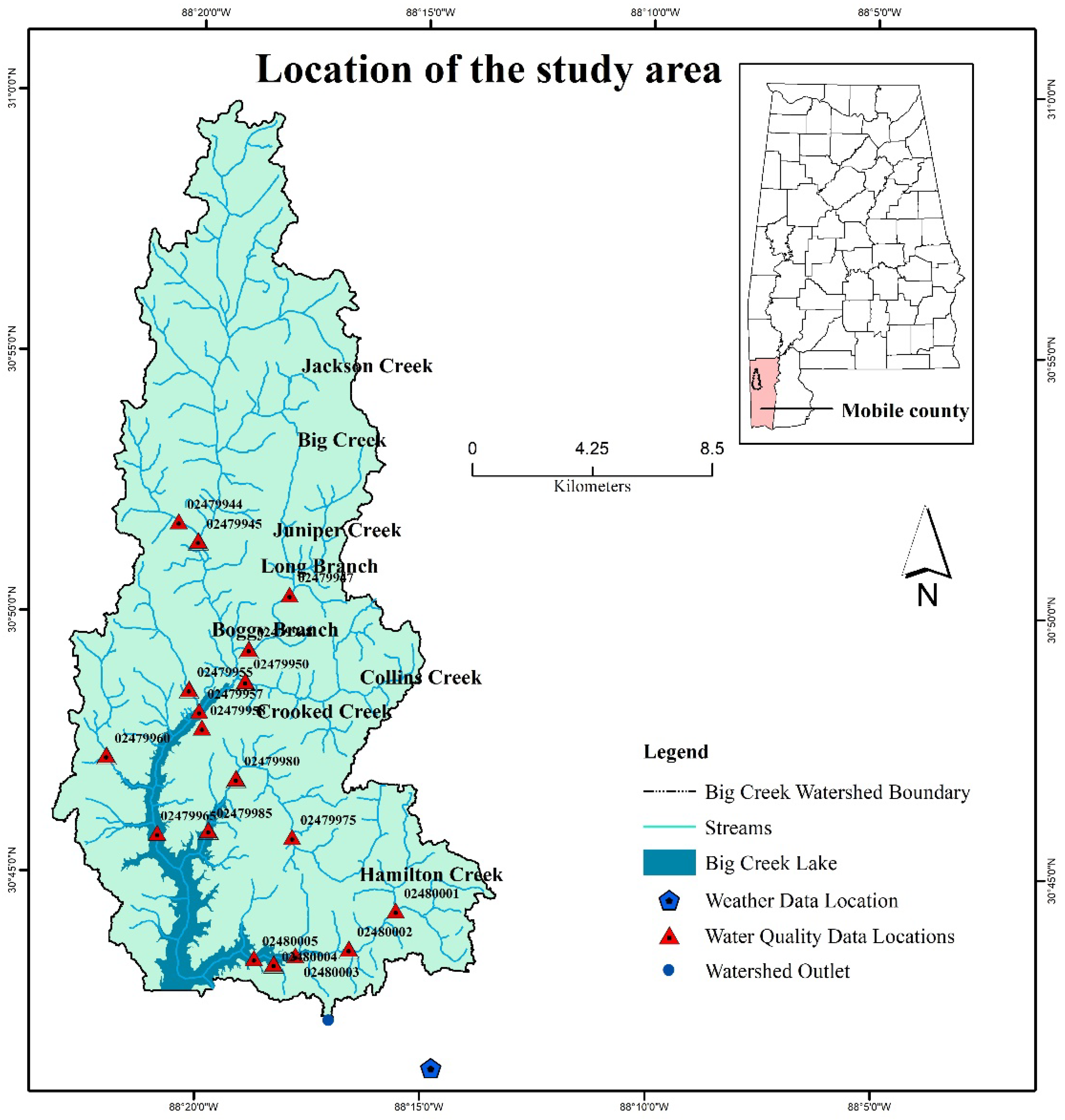
2.1. Study Area

Big Creek Lake has an area of 3600 acres and is a tributary-storage reservoir in Mobile County, located in southwest Alabama. Although the area of the lake itself is only 3600 acres, the watershed draining into it covers approximately 65,920 acres or 103 square miles [16,17]. Although Big Creek Lake watershed encompasses large areas in Mobile County, no large municipalities exist within the watershed; however, there are several smaller towns, including Wilmer and Semmes, located within the watershed boundaries. Figure 1 shows the location of the watershed, and the weather and water quality data stations. Big Creek Lake watershed lies within the Southern Hills District of the East Gulf Coastal Plain section of the Coastal Plain Physiographic Province in close proximity to the Gulf Coast. The Gulf of Mexico influences the subtropical climate of the watershed.

2.2. Data Required

Some spatial inputs are required to run the Soil Water Assessment Tool (SWAT) model, such as a digital elevation model (DEM) and associated topography, LULC, and soils of the study area [18,19]. In addition to these inputs, long-term weather data, soil property data, and discharge data are also necessary. The USGS National Map was the provider of the DEM datasets, which were downloaded from https://viewer.nationalmap.gov/basic/ (accessed on 28 March 2020). The spatial resolution is 10 m, which is a 1 arc-second (10 m × 10 m) pixel resolution. For LULC data, Landsat images obtained from the USGS data hub (https://earthexplorer.usgs.gov/ (accessed on 4 April 2020)) and same-seasonal images were chosen from 1990 to 2020 with minimum cloud cover to have the lowest atmospheric effects. Each LULC product was primarily based upon the classification of Landsat data. Classification was performed using the unsupervised approach. The resulting classification was then reclassified into water, forest, urban, agriculture, and rangeland. The SSURGO (Soil Survey Geographic Database) soil data were used because, according to the Natural Resource Conservation Service (NRCS), the SSURGO is the county soil data having the most detailed level. The soil data and information on related soil properties were obtained from https://websoilsurvey.sc.egov.usda.gov/App/WebSoilSurvey.aspx (accessed on 11 May 2020). From the National Oceanic and Atmospheric Administrations (NOAA) website, the daily rainfall, maximum and minimum temperatures, and average wind speed at one weather station in the study were obtained between 1990 and 2020. The daily stream flow data were obtained from the USGS National Water Information System: Web Interface. Water quality data are not available in daily or monthly intervals; rather its reporting is random.

2.3. SWAT Model Description

The SWAT is a physically based hydrologic model and requires physically based data [20]. The SWAT is a continuous-time, spatially distributed model designed to simulate water, sediment, nutrient, and pesticide transport at a catchment scale on a daily time step under different management practices [21]. Arc-SWAT is an extension of ArcGIS, as the SWAT is embedded in a GIS interface. SWAT2012 is evolved from AVSWAT, which is an extension of ArcView developed for an earlier version of SWAT2012. Some major components are used to run the SWAT model including weather, hydrology, different types of soil, plant growth, nutrients, pesticides, bacteria and pathogens, land use, and management practices. When running the SWAT model, a watershed or basin is divided into multiple sub-basins or sub-watersheds, and then each sub-basin or sub-watershed is further subdivided into multiple HRUs based on the DEM properties. HRUs are located in the sub-basin and comprise unique land use, soil, and slope characteristics. The Soil Conservation Services (SCS) curve number procedure (SCS, 1972) and Green and Ampt infiltration method (1911) are the two methods used by the SWAT model to estimate the surface runoff. In this study, the SCS curve number method was used to estimate surface runoff. Water is routed through the channel network using a variable storage routing method or the Muskingum routing method. In this study, Muskingum routing methods were used for surface runoff. Briefly, the SWAT partitions soil nitrogen (N) into five different N pools. Two of the pools are inorganic (ammonium-N [NH4-N] and nitrate-N [NO3-N]) and three pools are organic (active, stable, and fresh). Unlike N, soil phosphorous (P) in SWAT is divided into six pools (three minerals and three organics). The fresh organic phosphorus pool, and active and stable organic pool, are contributed to by the crop residue, and biomass and humus substances, respectively. The soil inorganic pool includes active, solution, and stable pools [22].

2.4. Uncertainty and Sensitivity Analysis

Sensitivity analysis is the identification of the sensitive parameters that have an important influence on the performance of the model, to ensure that adjustments will be precise. This operation was carried out using SWAT-CUP. This program was developed by the Swiss Federal Institute of Water Science and Technology (EAWAG), which specializes in SWAT calibration, validation, and uncertainty analysis. SWAT-CUP is a standalone program that links to SWAT’s output text files, and integrates five different optimization algorithms: Sequential Uncertainty Fitting (SUFI-2) [23], Generalized Likelihood Uncertainty Estimation (GLUE) [24], Parameter Solution (ParaSol) [25], Markov chain Monte Carlo (MCMC) [26,27,28], and Particle Swarm Optimization (PSO) [9]. Among these algorithms, SUFI-2 has the capacity to account for all the sources of uncertainty in the parameter ranges, such as uncertainty in driving variables (e.g., rainfall), conceptual model, parameters, and measured data [23]. For this reason, SUFI-2 was used in this study to analyze the sensitivity of the model.

2.5. SWAT Model Calibration, Validation and Evaluation

The calibration of the hydrological model is undertaken to optimize its predictive capacity by comparing its simulated values with the observed or actual values of the study area. Validation is the process of demonstrating the capability of making a sufficiently accurate simulation, which may vary based on the aim of a project [29]. In this study, a five-year warm-up period, that is, from 1986 to 1990, was used. The calibration and validation periods were equal for stream flow, nitrogen, and phosphorus. Predicted and observed values of streamflow and nutrient loadings at the watershed outlet were compared to determine whether the objective function satisfactorily involves running a model using the parameters during the calibration. The results from the different periods of calibration were compared to determine whether the model meets confidence limits. The model validation was performed with the same SWAT parameter values calibrated without any further alterations. The performance of the model in the simulation was evaluated by Nash–Sutcliffe Efficiency (NSE), Percent of Bias (PBIAS), and the Coefficient of Correlation (R2), which are most commonly used and are proposed [30].

3. Results

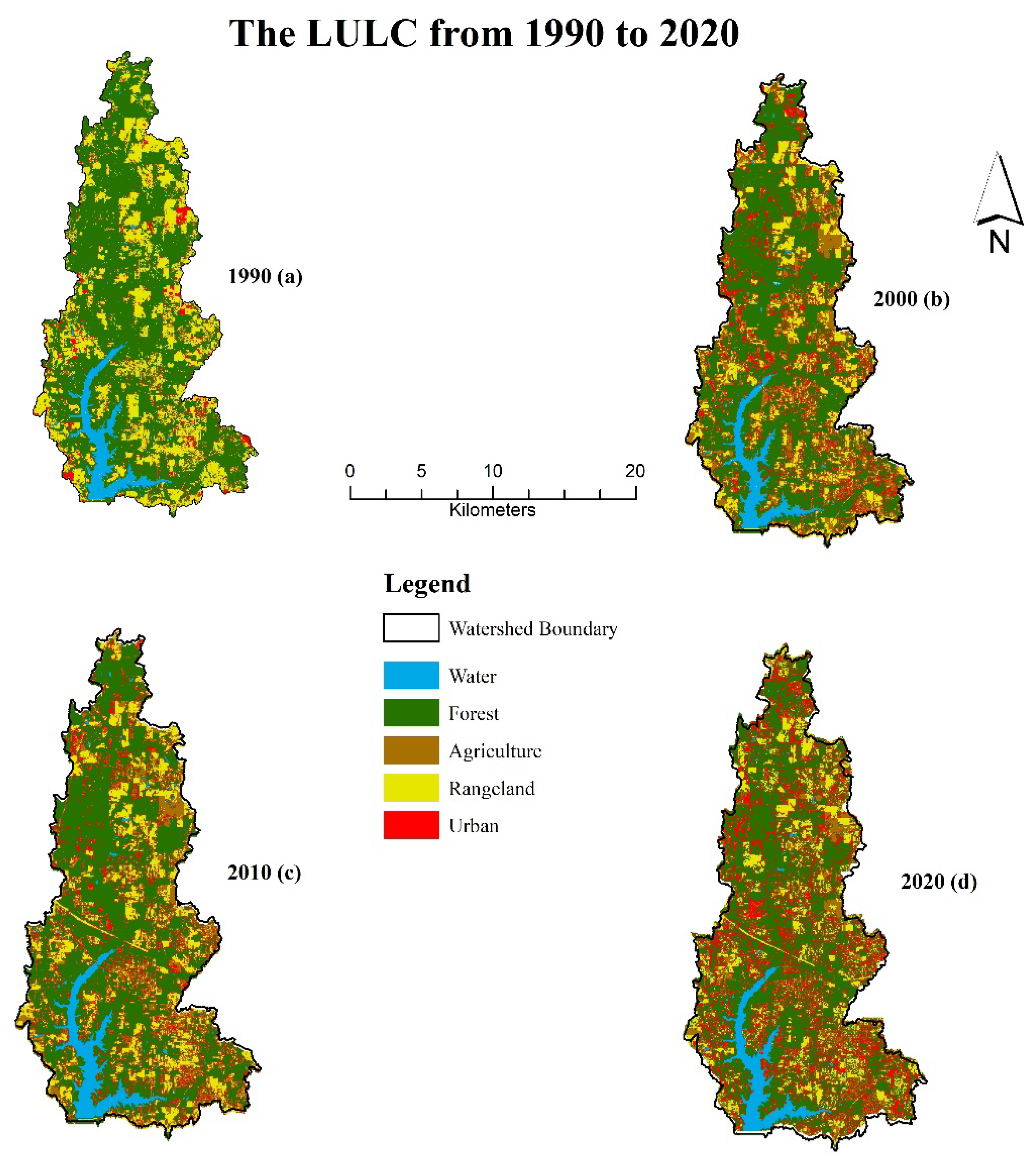
3.1. Land Use and Land Cover (LULC) Change

Figure 2 shows the land use over the period. Forest was one of the main land uses of the watershed and achieved a large percentage. From 1990 to 2000, almost 60% of the watershed area was forest land. However, after one decade (2010), forest area was reduced by about 10%. A total of 11,482.80 acres of forest area were transformed into other LULC categories over a 30-year period. By comparison, urban areas increased (3350 acres) in the past three decades, showing an increment of 1293 acres from 1990 to 2000, 632 acres from 2000 to 2010, and 1423 acres from 2010 to 2020. Agricultural land increased (11,045 acres) and rangeland decreased (2542 acres) in the last three decades. From 1990 to 2000, agricultural land increased, but from 2000 to 2010 it decreased, and, in the last decade, it increased by about 10,510 acres. The LULC time series analysis between 1990 and 2020 indicates an expansion in the agricultural land and an increase in urban area, with a reduction in forest land and rangeland. Forest area changed to rangeland and urban areas, by approximately 8086 and 3905 acres, respectively, in the last three decades. Agricultural land transformed into rangeland (852 acres) and urban area (674 acres), mostly from 1990 to 2020. Meanwhile, during the same period, rangeland changed into the agricultural area (5380 acres) and urban area (2080 acres).

3.2. Sensitivity Analysis

Table 1 represents the fifteen parameters used to calibrate and validate the stream flow. Based on sensitivity analysis, fifteen parameters were used, such as curve number (CN), biological mixing efficiency (BIOMIX), Manning’s “n” value for overland flow (OV_N), peak rate adjustment factor (PRF), exponent parameter for calculating sediment re-entrained in channel sediment routing (SPEXP), USPE equation (USLE_P), plant and soil evaporation factor (ESCO and EPCO), and groundwater (ALPHA_BF, GW_DELAY, GW_REVAP, and RCHRG_DP). SOL_LABP, SOL_ORGP, LAT_ORGN, and SOL_ORGN were used to calibrate the nitrogen and phosphorus flow in the watershed.
Table 2 ranks the parameters based on the t-stat and p-value, using the highest absolute value of the t-stat and the lowest value of the p-value, the highest influence of that parameter, and vice versa. Based on these values, SOL_AWC, OV_N, and RCHRG_DP are the most effective parameters, and ESCO, ULSE_P, and BIOMIX have less impact on the calibration and validation of the model.

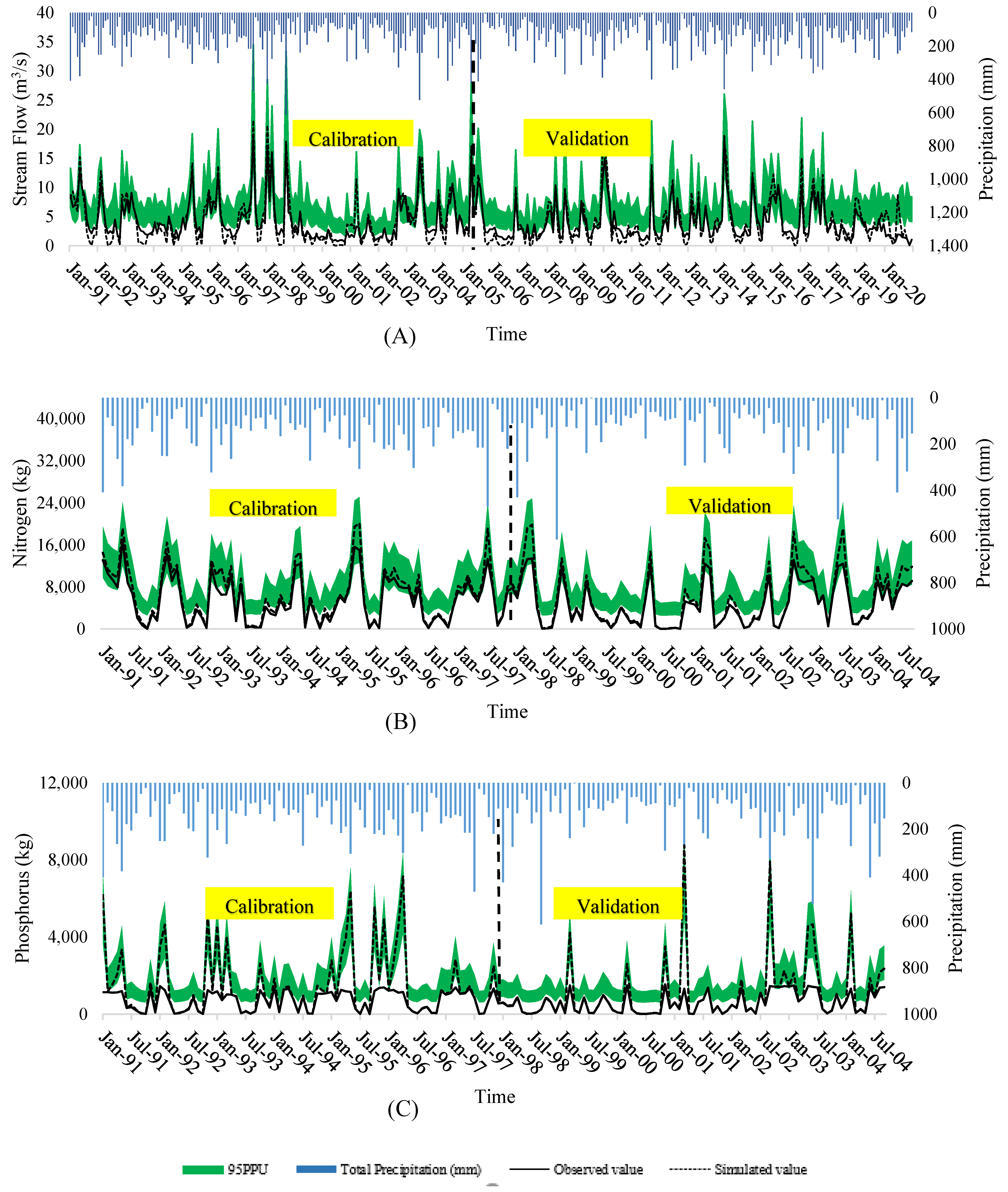
3.3. SWAT Model Calibration and Validation

Figure 3A–C show the observed and simulated monthly stream flow, total nitrogen, and phosphorus, respectively. The differences in the average monthly observed and simulated values of stream flow were less than 1%. The R2, NSE, and PBIAS values for streamflow for the calibration and validation periods are listed in Table 3. Based on the classified value stated by Moriasi et al. (2015), the SWAT model showed a very good level in the NSE for calibration (0.77) and validation (0.73). Adjustment between the observed, calibrated, and validated stream flow reached a good level, having an R2 of 0.81 for both calibration and validation. A good classification was obtained for PBIAS, with values of 10.7% and 15.4% for calibration and validation, respectively. According to the classification by Moriasi et al. (2007), the SWAT model calibrated and validated the nitrogen and phosphorus satisfactorily in the determination coefficient (Table 3).

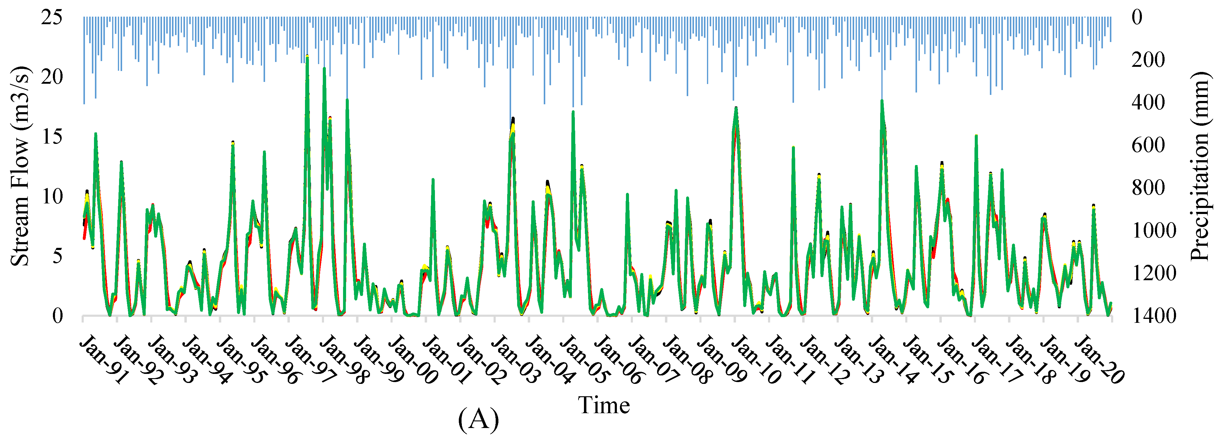
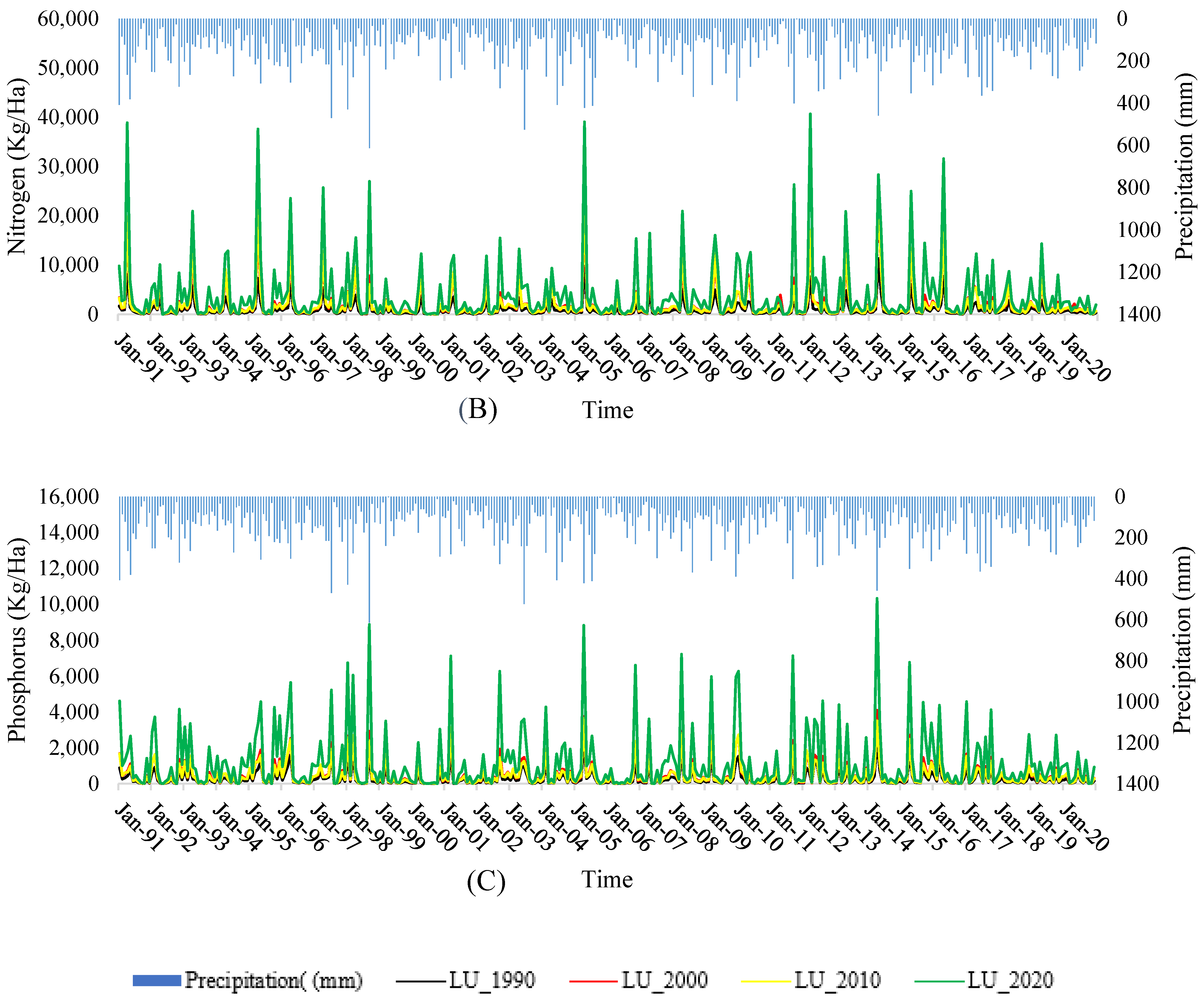
3.4. Stream Flow, Nitrogen, Phosphorus of Different LU Scenarios

The relationship between stream flow and LULC, nitrogen and LULC, and phosphorus and LULC is shown by Figure 4A–C respectively. The effect of the stream flow, nitrogen, and phosphorus was estimated for the 30-year study period (1990–2020) by running the LU_1990, LU_2000, LU_2010, and LU_2020 scenarios. The greatest differences in the total stream flow between LU_1990 and LU_2000, and between LU_2010 and LU_2020, were decreases of around 12 and 21 m3/s, respectively. These differences from 1990 to 2000 were characterized by increasing urban area and agricultural land by 1293 and 894 acres, respectively, and increasing stream flows from 2010 to 2020 were influenced by increasing agricultural land and urban area, by 10,510 acres and 1423 acres, respectively. Moreover, comparing LU_1990 and LU_2020, total monthly stream flow increased about 38 m3/s, which can be explained by changes in LULC, namely, increasing agricultural land by 11,045 acres and urban area by 3350 acres. Moreover, the same behavior was noticed in the stream flow between LU_2000 and LU_2010, by increasing stream flow by about 5 m3/s. Both nitrogen and phosphorus had an increasing trend over the last three decades. From 1990 to 2020, nitrogen increased by 1,136,919 kg, and from 2010 to 2020, nitrogen increased by 768,893 kg; these increases can be explained by the increase in agricultural land, by about 11,045 and 10,510 acres. respectively. From 1990 to 2020, phosphorus increased by 324,467 kg, and most of the increase in phosphorus (around 253,975 kg) occurred in the past decade (2010–2020) (Figure 4B,C).

4. Discussion

This study shows that changes in LULC that occurred from 1990 to 2020 in the Big Creek Lake watershed were characterized by a substantial increase in agricultural land and expansion of the urban area. These results complement the study of the comparison of temporal images of LULC for the watershed conducted by [16]. This study found that an urban area expansion occurred, and the percentage increase in high and low residential areas was 2.3% and 10.1%, respectively. According to [17], the percentage of agricultural lands is highest in the Crooked Creek sub-basin, accounting for over 41% of the sub-basin. Much of the land in the sub-basin is designated as row crops. Hamilton Creek has also the highest percentage of agricultural land (36.1%). Potential sources of nutrients in the Big Creek Lake watershed are from nonpoint contributions associated with fertilizer applications on agricultural and residential land, livestock wastes, residential runoff, failing septic systems, and contaminated groundwater. No known point sources are located in the Big Creek Lake watershed. According to [17], the total annual nutrient loads at Big Creek Lake for the 1991 water year were 118,000 kg for total nitrogen and 5245 kg for total phosphorus. As population growth continues, and hence the conversion of forested areas to agriculture and urban areas, loadings of nutrients are expected to increase because most of the land is converted to urban areas. A study conducted by [15] and prepared in cooperation with MAWSS concluded that total nitrogen (except for Long Branch), total Kjeldahl nitrogen (except for Hamilton Creek), total organic nitrogen (except for Boggy Branch), ammonia (except for Long Branch), total inorganic nitrogen, and total phosphorus (except for Long and Boggy Branches) exhibited significant, positive relationships with streamflow, which indicate the dominant source of nutrient input to the watershed is from nonpoint sources. The more residential and agricultural sub-basins of Crooked Creek and Hamilton Creek, however, yielded over twice the total phosphorus per hectare of land use. Crooked and Hamilton Creek sub-basins also had higher total inorganic nitrogen yields. These results complement the present study, which found that, over time, the stream flow increases with the increase in total nitrogen and phosphorus. This increasing nature has a positive relationship with the increase in agricultural land and urban areas. A significant, positive relationship between streamflow and nutrient concentration indicates that nonpoint sources are the dominant source of the inputs. Different land-use practices contribute different levels of nutrients by nonpoint sources.

5. Conclusions

The SWAT model is highly significant and useful because it can be used to predict future hydrological responses. The total stream flow grew by 38 m3/s, and total nitrogen and phosphorus increased by about 113,619 and 324,467 kg, respectively, over the past three decades. This study quantified the impact of the changes in LULC on the water balance components and water quality. The results can be used by decision makers and public policy makers for future projections in terms of LULC changes.

Author Contributions

Conceptualization, E.A.E.; methodology, E.A.E.; software, E.A.E.; validation, E.A.E.; formal analysis, E.A.E.; data curation, E.A.E.; writing—original draft preparation, E.A.E.; writing—review and editing, E.A.E. and L.J.M.; visualization, E.A.E.; supervision, L.J.M. All authors have read and agreed to the published version of the manuscript.

Funding

This research received no external funding.

Institutional Review Board Statement

Not applicable.

Informed Consent Statement

Not applicable.

Conflicts of Interest

The authors declare no conflict of interest.

References

  1. Zhang, M.; Liu, N.; Harper, R.; Li, Q.; Liu, K.; Wei, X.; Ning, D.; Hou, Y.; Liu, S. A global review on hydrological responses to forest change across multiple spatial scales: Importance of scale, climate, forest type and hydrological regime. J. Hydrol. 2017, 546, 44–59. [Google Scholar] [CrossRef] [Green Version]
  2. Gao, G.; Fu, B.; Wang, S.; Liang, W.; Jiang, X. Determining the hydrological responses to climate variability and land use/cover change in the Loess Plateau with the Budyko framework. Sci. Total Environ. 2016, 557, 331–342. [Google Scholar] [CrossRef] [PubMed]
  3. Jarsjö, J.; Asokan, S.M.; Prieto, C.; Bring, A.; Destouni, G. Hydrological responses to climate change conditioned by historic alterations of land-use and water-use. Hydrol. Earth Syst. Sci. 2005, 16, 1335–1347. [Google Scholar] [CrossRef] [Green Version]
  4. Wei, X.; Zhang, M. Quantifying streamflow change caused by forest disturbance at a large spatial scale: A single watershed study. Water Resour. Res. 2010, 46, 1–15. [Google Scholar] [CrossRef]
  5. Pitman, A.J. The evolution and revolution in land surface schemes designed for climate models. Int. J. Climatol. 2003, 23, 479–510. [Google Scholar] [CrossRef]
  6. Sy, S.; Noblet-Ducoudré, N.D.; Quesada, B.; Sy, I.; Dieye, A.M.; Gaye, A.T.; Sultan, B. Land-surface characteristics and climate in West Africa: Models’ biases and impacts of historical anthropogenically-induced deforestation. Sustainability 2017, 9, 1917. [Google Scholar] [CrossRef] [Green Version]
  7. Sertel, E.; Robock, A.; Ormeci, C. Impacts of land cover data quality on regional climate simulations. Int. J. Climatol. 2010, 30, 1942–1953. [Google Scholar] [CrossRef]
  8. Lee, S.-J.; Berbery, E.H. Land cover change effects on the climate of the La Plata Basin. J. Hydrometeorol. 2012, 13, 84–102. [Google Scholar] [CrossRef]
  9. Marland, G. The climatic impacts of land surface change and carbon management, and the implications for climate-change mitigation policy. Clim. Policy 2003, 3, 149–157. [Google Scholar] [CrossRef] [Green Version]
  10. Welde, K.; Gebremariam, B. Effect of land use land cover dynamics on hydrological response of watershed: Case study of Tekeze Dam watershed, northern Ethiopia. Int. Soil Water Conserv. Resour. 2017, 5, 1–16. [Google Scholar] [CrossRef]
  11. Wang, H.; Sun, F.; Xia, J.; Liu, W. Impact of LUCC on streamflow based on the SWAT model over the Wei River basin on the Loess Plateau in China. Hydrol. Earth Syst. Sci. 2017, 21, 1929–1945. [Google Scholar] [CrossRef] [Green Version]
  12. Lin, B.; Chen, X.; Yao, H.; Chen, Y.; Liu, M.; Ga, L.; James, A. Analyses of landuse change impacts on catchment runoff using different time indicators based on SWAT model. Ecol. Indic. 2015, 58, 55–63. [Google Scholar] [CrossRef]
  13. Nie, W.; Yuan, Y.; Kepner, W.; Nash, S.M.; Michael, J.; Caroline, E. Assessing impacts of land use and land cover changes on hydrology for the upper San Pedro watershed. J. Hydrol. 2011, 407, 105–114. [Google Scholar] [CrossRef]
  14. Gassman, P.W.; Reyes, M.R.; Green, C.H.; Arnold, J.G. SWAT peer-reviewed literature: A review. In Proceedings of the 3rd International SWAT Conference, Zurich, Switzerland, 13–15 July 2005. [Google Scholar]
  15. Gill, A.C.; McPherson, A.K.; Moreland, R.S. Water Quality and Simulated Effects of Urban Land-Use Change in J.B. Converse Lake Watershed, Mobile County, Alabama, 1990–2003: U.S. Geological Survey Scientific Investigations Report; United States Geological Survey: Reston, VA, USA, 2005; pp. 2005–5171. 110p.
  16. Mobile Area Water and Sewers Systems (MAWSS). Water System. 2011. Available online: http://www.mawss.com/waterSystem.html (accessed on 31 December 2020).
  17. Journey, C.A.; Gill, A.C. Assessment of water-quality conditions in the J.B. Converse Lake Watershed, Mobile County, Alabama, 1990–1998. U.S. Geological Survey Water-Resources Investigations Report 01-4225. Available online: http://pubs.er.usgs.gov/publication/wri014225 (accessed on 28 December 2020).
  18. Monteith, J.L. Evaporation and environment. Symp. Soc. Exp. Biol. 1965, 19, 205–234. [Google Scholar] [PubMed]
  19. Arnold, J.G.; Kiniry, J.R.; Srinivasan, R.; Williams, J.R.; Haney, E.B. Soil and Water Assessment Tool Input/Output Documentation; TR-439; Texas Water Resources Institute: College Station, TX, USA, 2012; pp. 1–650. [Google Scholar]
  20. Jacobs, J.H.; Srinivasan, R. Effects of curve number modification on runoff estimation using WSR-88D rainfall data in Texas watersheds. J. Soil Water Conserv. 2005, 60, 274–278. [Google Scholar]
  21. Jain, M.; Sharma, S.D. Hydrological modeling of Vamshadara River Basin, India using SWAT. In Proceedings of the International Conference on Emerging Trends in Computer and Image Processing (ICETCIP-2014), Pattaya, Thailand, 15–16 December 2014. [Google Scholar]
  22. Chaubey, I.; Miglizccio, K.W.; Green, C.H.; Arnold, J.G.; Srinivasan, R. Phosphorus Modeling in Soil and Water Assessment Tool (SWAT) Model. In Modeling Phosphorus in the Environment; Radcliffe, D.E., Cabrera, M.L., Eds.; CRC Press: New York, NY, USA, 2007; pp. 163–188. [Google Scholar]
  23. Abbaspour, K.C.; Yang, J.; Maximov, I.; Siber, R.; Bogner, K.; Mieleitner, J.; Zobrist, J.; Srinivasan, R. Modelling hydrology and water quality in the pre-alpine/alpine Thur watershed using SWAT. J. Hydrol. 2007, 333, 413–430. [Google Scholar] [CrossRef]
  24. Beven, K.; Binley, A. The future of distributed models: Model calibration and uncertainty prediction. Hydrol. Processes 1992, 6, 279–298. [Google Scholar] [CrossRef]
  25. Van Griensven, A.; Meixner, T. Methods to quantify and identify the sources of uncertainty for river basin water quality models. Water Sci. Technol. 2006, 53, 51–59. [Google Scholar] [CrossRef]
  26. Kuczera, G.; Parent, E. Monte Carlo assessment of parameter uncertainty in conceptual catchment models: The Metropolis algorithm. J. Hydrol. 1998, 211, 69–85. [Google Scholar] [CrossRef]
  27. Marshall, L.; Nott, D.; Sharma, A. A comparative study of Markov chain Monte Carlo methods for conceptual rainfall-runoff modeling. Water Resour. Res. 2004, 40, 1–11. [Google Scholar] [CrossRef]
  28. Vrugt, J.A.; Gupta, H.V.; Bouten, W.; Sorooshian, S. A shuffled complex evolution Metropolis algorithm for optimization and uncertainty assessment of hydrologic model parameters. Water Resour. Res. 2003, 39, 1–14. [Google Scholar] [CrossRef] [Green Version]
  29. Refsgaard, J.C. Parameterization, calibration, and validation of distributed hydrological models. J. Hydrol. 1997, 198, 69–97. [Google Scholar] [CrossRef]
  30. Moriasi, N.; Daniel, G.W.; Pai Naresh, M.; Prasad, D. Hydrologic and water quality models: Performance measures and evaluation criteria. Trans. Soc. Agric. Biol. Eng. (ASABE) 2015, 58, 1763–1785. [Google Scholar] [CrossRef] [Green Version]
Figure 1. Location of the study area.
Environsciproc 15 00009 g001
Figure 2. LULC for 1990 (a), 2000 (b), 2010 (c), and 2020 (d).
Environsciproc 15 00009 g002
Figure 3. Observed vs. simulated stream flow (m3/s) from 1991 to 2020 (A), total nitrogen (Kg/Ha) from 1991 to 2004 (B), and total phosphorus (Kg/Ha) (C) from 1991 to 2004.
Environsciproc 15 00009 g003
Figure 4. Simulated monthly flow (m3/s) (A), total nitrogen (Kg/Ha) (B), and total phosphorus (Kg/Ha) (C) between 1991 and 2020 for different LULC scenarios (LU_1900, LU_2000, LU_2010, and LU_2020).
Environsciproc 15 00009 g004aEnvironsciproc 15 00009 g004b
Table 1. Model parameters and their descriptions in surface flow, total nitrogen, and phosphorus calculations.
ParameterParameter DescriptionFitted ValueMinimum ValueMaximum Value
ADJ_PKRPeak rate adjustment factor for sediment routing in sub watershed20.52
ALPHA_BFBaseflow alpha factor (days)0.101
BIOMIXBiological mixing efficiency0.201
CNCurve numberDecrease 20%3598
EPCOPlant evaporation compensation factor0.9501
ESCOSoil evaporation compensation factor101
GW_DELAYGroundwater delay time (days)200500
GW_REVAPGroundwater “revap” coefficient0.020.020.2
OV_NManning’s “n” value for overland flow “n” value for overland flow10.0130
PRFPeak rate adjustment factor for sediment routing in the main channel101
RCHRG_DPDeep aquifer percolation factor0.0501
SOL_AWCAvailable water capacity of soil layer0.701
SOL_KSaturated hydraulic conductivity0.202000
SPEXPExponent parameter for calculating sediment retrained in channel sediment routing1.511.5
USLE_PUSLE equation support practice factor101
SOL_LABPInitial soluble P concentration in sol layer0.010100
SOL_ORGPInitial organic P concentration in sol layer0.010100
LAT_ORGNOrganic N in the baseflow0.010200
SOL_ORGNInitial organic N concentration in the soil layer0.01010
Table 2. Sensitive parameters ranking based on t-Stat and p-Value.
Parameter Namet-Statp-ValueParameter Namet-Statp-Value
r__ESCO.bsn−0.2152787270.829640698r__EPCO.bsn1.1156966140.265105646
r__USLE_P.mgt−0.2269508550.820557782r__CN2.mgt−1.3337777870.18290399
r__BIOMIX.mgt0.2270964860.820444606r__ADJ_PKR.bsn−1.4436127370.149494876
r__ALPHA_BF.gw−0.2788636190.780468599r__PRF_BSN.bsn−1.9480625490.051985146
r__SOL_K().sol0.6714554550.502250766r__RCHRG_DP.gw−1.9949934780.046603828
r__GW_REVAP.gw−0.7288523670.466444494r__OV_N.hru−2.8623650890.004387183
r__GW_DELAY.gw0.8466683730.39759842r__SOL_AWC().sol−38.31789330
r__SPEXP.bsn−0.9693464870.332856487---
Table 3. Statistical evaluation of the model for calibration and validation time periods.
R2NSEPBIAS
CalibrationValidationCalibrationValidationCalibrationValidation
Stream Flow0.810.810.770.73−10.715.4
Nitrogen0.750.770.620.659.34−3.45
Phosphorus0.50.540.340.24−20.45−21.76
Publisher’s Note: MDPI stays neutral with regard to jurisdictional claims in published maps and institutional affiliations.

