Article

Determination of Dynamic Characteristics for Predicting Electrical Load Curves of Mining Enterprises †

by
Denis Anatolievich Ustinov
and
Konstantin Alekseevich Khomiakov
*
Department of Electric Power and Electromechanics, St. Petersburg Mining University, 199106 St. Petersburg, Russia
*
Author to whom correspondence should be addressed.
This paper is an extended version of our conference paper: Ustinov, D.A, Khomiakov, K.A. “Comprehensive assessment of factors determining electricity load curves concerning enterprises of mineral resource sector.” In Proceedings of the Physical Studies and Digitalization in Mining Engineering (IPDME), St. Petersburg, Russia, 23−24 April 2020.
Electricity 2022, 3(2), 162-181; https://doi.org/10.3390/electricity3020010
Submission received: 17 January 2022 / Revised: 5 March 2022 / Accepted: 29 March 2022 / Published: 8 April 2022

Abstract

:
The calculation of electrical loads is the first and most significant stage in the design of the power supply system. It is essential to make the right choice when choosing the power electrical equipment: transformers, power lines, and switching devices. Underestimation or overestimation of the calculated values can lead to large losses and an increase in capital costs. Therefore, the reliability of the results plays a key role. The use of energy-saving technologies and energy-efficient electrical equipment leads to a change in the nature and level of power consumption, which must be taken into account when determining the electrical loads. The existing methods leave out dynamic characteristics of electrical load curves, so the calculated values are overestimated by up to 40%. This study shows a load calculation method with the normalized correlation functions and its parameters at the level of the individual and group electricity consumers. As a result, the difference between the calculated and experimental values does not exceed 5%.

1. Introduction

The existing high energy utilization rates in the energy sector mean that the required improvements must be made in terms of returns on capital investments and material costs. Currently, the consumption of electricity by industrial enterprises in certain regions of Russia can reach about 44% (in the Nenets Autonomous Area). For example, the Ural Federal District is one of the richest mineral regions in Russia, with a share of electricity consumption by industrial enterprises constituting about 30% and with the likelihood of such consumption increasing due to the active development of this region and the construction of new industrial enterprises [1]. The construction and further operation of any industrial enterprise is preceded by the design stage, involving the definition of the key characteristics of each system and the design of the power supply system (PSS). The efficiency of the PSS is determined by the reliable evaluation of the characteristics of electrical loads, with the calculated results then shown in graphs [2]. This is due to the fact that the calculated characteristics electrical loads provide information to inform the solutions for most of the technical and economic issues in the design stage.
It should also be noted that the issues regarding energy efficiency and energy savings are very acute, and the measures taken to achieve certain goals are widely implemented in all production cycles, meaning that it is important to take these changes into consideration when calculating electrical loads by using probabilistic calculation methods [3].
Reference [4] reviewed how the need for efficient electrical energy consumption has greatly expanded in the process industries. The article dealt with industrial enterprises for the recognition of electricity consumption in a two-echelon supply model with a stochastic lead-time demand and imperfect production, while considering the distribution-free approach. Reference [5] discussed the impact of electric energy on production cost recovery, transport discounts and process quality improvement in two algorithms are developed using an analytical approach to obtain the optimal solution. With the increase in the varieties products and the increasing uncertainty about product demand, the production preparation time is a significant factor in addressing these issues. The basic calculation methods applied today, such as the method of ordered diagrams (MOD) [6] and the modified statistical method (MSM) [7], lead to significant errors in estimating the design loads, as shown in References [7,8]. This is due to the fact that the applied methods are static modeling methods that involve uninformative mathematical model, while the indicated design characteristics can solve only a very limited range of technical and economic issues; as a consequence, the efficiency of the PSS is reduced. As such, increasing the energy efficiency of mineral resource enterprises by improving the methods for calculating electrical loads is an urgent task, as these initial datasets are used in design stage.
The methods for calculating electrical loads used currently in our country and abroad refer to probabilistic methods based on a mathematical model of the “random variable” [9,10]. It should be noted that we are talking about methods of raising mining enterprises and not about load forecasting based on an analysis of the current situation, and, for example, by using neural networks to predict both long-term and short-term load electrical curves [11]. The basis for all further research in the field of calculating electrical loads and, in fact, the first method based on the principles of the probability of a random process, is the statistical method; there is no need to dwell separately on the shortcomings, because they have already been repeatedly described in Reference [8].
The statistical method was replaced by the MOD [6], which made it possible to reduce errors in the estimation of electrical loads by creating a database of initial data of individual load schedules, but still remained insufficiently reliable; this is due to several shortcomings, especially the following: discrepancy between the design technological modes and the actual operating modes [12].
Today, all mining enterprises are designed by using an MSM [7]. Developed more than 25 years ago, these methods are the basis of approved methods for calculation of electrical loads [13]. Such a long break in research can be explained by the sufficient reliability of the MSM, combined with the simplicity of performing engineering calculations, but the last few years have been practically associated with a revolution in the mining and processing industry, increasing the automation of technological processes through the use of modern energy-efficient equipment [14,15]. Moreover, the effect of such changes must be taken into account, including in the calculation methods [16].
Separately, it is worth mentioning the alternative calculation methods considered in the works of Stepanova [17]; the main advantage of the method under consideration is the consideration of correlation dependencies both at the level of individual and group loads, as well as additional calculation of dynamic characteristics [18]. At the same time, the disadvantages include a small base of initial data on consumers, which, in turn, does not allow a reliable analysis of this method applied to consumers at mining enterprises, as well as the lack of accounting from the introduction of modern means to improve energy efficiency [19].
Table 1 presents the contributions to this paper.

2. Problem Definition, Notation, and Assumptions

2.1. Problem Definition

An analysis of the MSM and MOD showed differences in the reference and actual values of the utilization factors in determining the calculated electrical loads of a conveyor unit with and without the use of a variable-frequency drive (VFD) (Table 2 and Table 3).
The discrepancy between the reference values and the actual value of the utilization factor ( k u ) is about 35%, which goes beyond the range of permissible values. It should be noted that the existing database of coefficients does not take into account the usage of equipment with VFD [6,20].
Studies on the methods used for calculating electrical loads abroad have shown their similarities with the method of ordered diagrams and the statistical method. First of all, this is shown by the utilization factor, k u ; the demand factor, k d ; and the peak coincidence factor, k M [8,21]. Unfortunately, this approach to determining the key parameters of a power supply system (PSS) has proven its inefficiency due to overestimating the calculated values [22]. When examining the indicators of power consumption of operating enterprises, the obtained calculated maximum loads, according to foreign methods, exceed the actual values by 40–60%. The same values were obtained by using the method of ordered diagrams. The situation is better with the use of the modified statistical method, the description of which is presented at the beginning of this section, whereby the obtained calculated values exceed the actual values by 20–40% [15].
The overestimation of the calculated values is associated with disadvantages that are inherent in all of the methods under study. The detailed analysis carried out revealed the main disadvantages, which are shown in Table 4.

2.2. Notation

Therefore, just a revision of the estimated coefficients of existing methods is not enough to increase the reliability of the calculated values [6]. This is due to the fact that the applied methods are static modeling methods that involve uninformative mathematical model, while the indicated design characteristics can solve only a very limited range of technical issues. Moreover, an increase in the number and accuracy of the calculated characteristics is possible through the additional calculation of dynamic characteristics [16].
It should be noted that forecasting of electrical loads based on any type of probabilistic forecasting, for example, the use of neural networks, is best suited for the operation of the electrical complex of an enterprise; however, it is completely unsuitable for design [23].

2.3. Assumptions

The purpose of this paper is to increase the reliability of the calculated values through the applied method, which differs from classical methods. Such a calculation will help to make a right choice of power and switching electrical equipment for distribution and protection, which will reduce material inputs.
In summary, the significant contributions of this paper are as follows:
  • Determination of dynamic characteristics for predicting electrical load curves of mining enterprises and expanding the database containing the source data, as well as determining the difference in the characteristics of the same type of curves, using means to improve energy efficiency and without (Section 3).
  • Development of a methodology for the transition from individual load schedules to group ones and presentation of a calculation algorithm, taking into account the consideration of two laws of probability distribution (Section 4).
  • Carrying out a comparative analysis of existing classical calculation methods and the presenting a new method that makes it possible to take into account equipment, using means to improve energy efficiency (Section 5).

3. Dynamic Characteristics of Electrical Load Curves

As such, when determining the calculated loads, it is also necessary to take into account dynamic characteristics, such as peaks and valleys, surges and load dips, and load fluctuations, which will contribute to forecasting calculations of electrical loads with a higher confidence probability. It becomes possible by using a dynamic modeling method, such as the hierarchical–structural method (HSM) [24].
The method is realized for load curves of general-purpose industrial and special industrial consumers, and the base of the method is an extended database containing the source data with additional characteristics (Table 5), such as the normalized correlation function (NCF) and its parameters presented in the Table 5. The necessity of using additional characteristics is connected to a fundamental change of the initial information about the individual load curves of the consumers. Physically, the NCF describes the probabilistic causation for the sequence of ordinates of the random process of changing the load, and due to the fact that the technological processes in mining enterprises have a steady-state mode of operation, the load curves are stationary [25].
Our analysis of the literary sources [8,16,26] showed that the correlation functions (CF) for all general-purpose industrial and special industrial consumers can be approximated by using the following analytical expressions:
K ( τ ) = D p e x p ( α | τ | ) ;
K ( τ ) = D p e x p ( α | τ | ) C o s ω 0 τ ;
K ( τ ) = D p e x p ( α | τ | ) ( C o s ω 0 τ α ω 0   s i n ω 0 | τ | ) ;
K ( τ ) = D p e x p ( α | τ | ) ( C o s ω 0 τ + α ω 0   s i n ω 0 | τ | ) ;
where D p e x p is the variance of an individual electrical load curve (ELC), the parameter α characterizes the attenuation of correlations between the ordinates of the initial ELC, and ω 0 is the natural frequency of oscillations of the CF, due to the repeatability of technological operations. The main idea of this study is to identify differences in the NCF and its parameters for the same consumers, both with and without using means to improve energy efficiency.
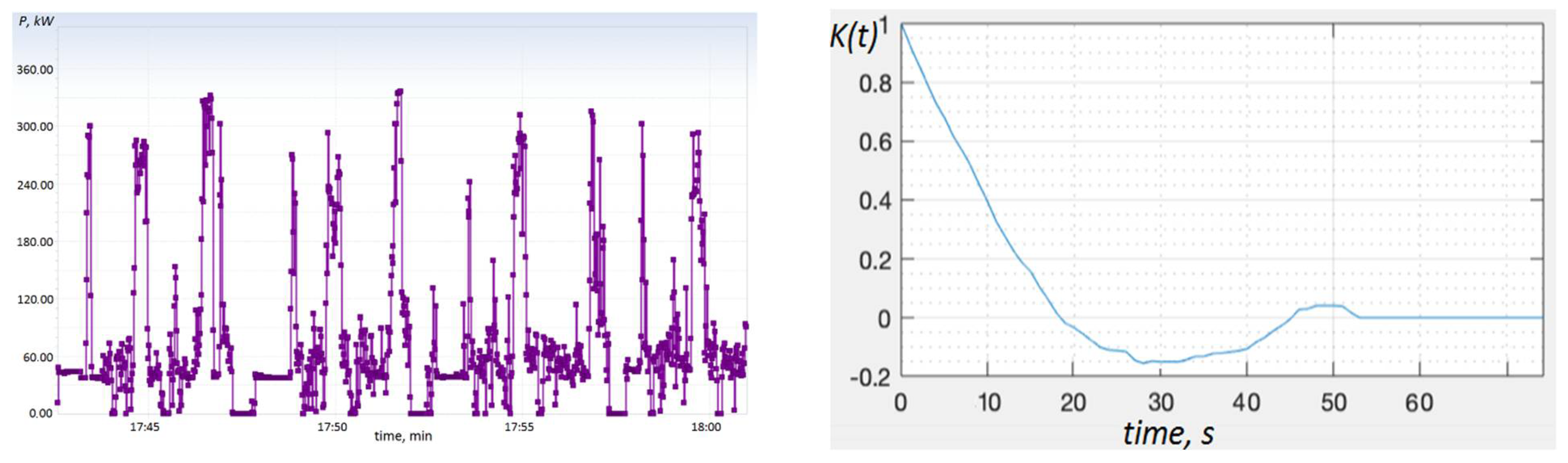
Experimental studies aimed at determining the NCF and its parameters of the electrical load curves were carried out in operating mining enterprises, the main consumers of which are general-purpose industrial consumers. The load curves were compared with and without using energy-efficiency means—in this case, with and without the use of a variable-frequency drive. The initial curves and step-wise determination of the type and parameters of the NCF for a conveyor unit with power motor of p n o m = 250   kW are given by way of example. Earlier, in Reference [24], the authors described a detailed algorithm for determining the NCF, so this article presents only the main points.
  • Determination of the average load value (Table 6).
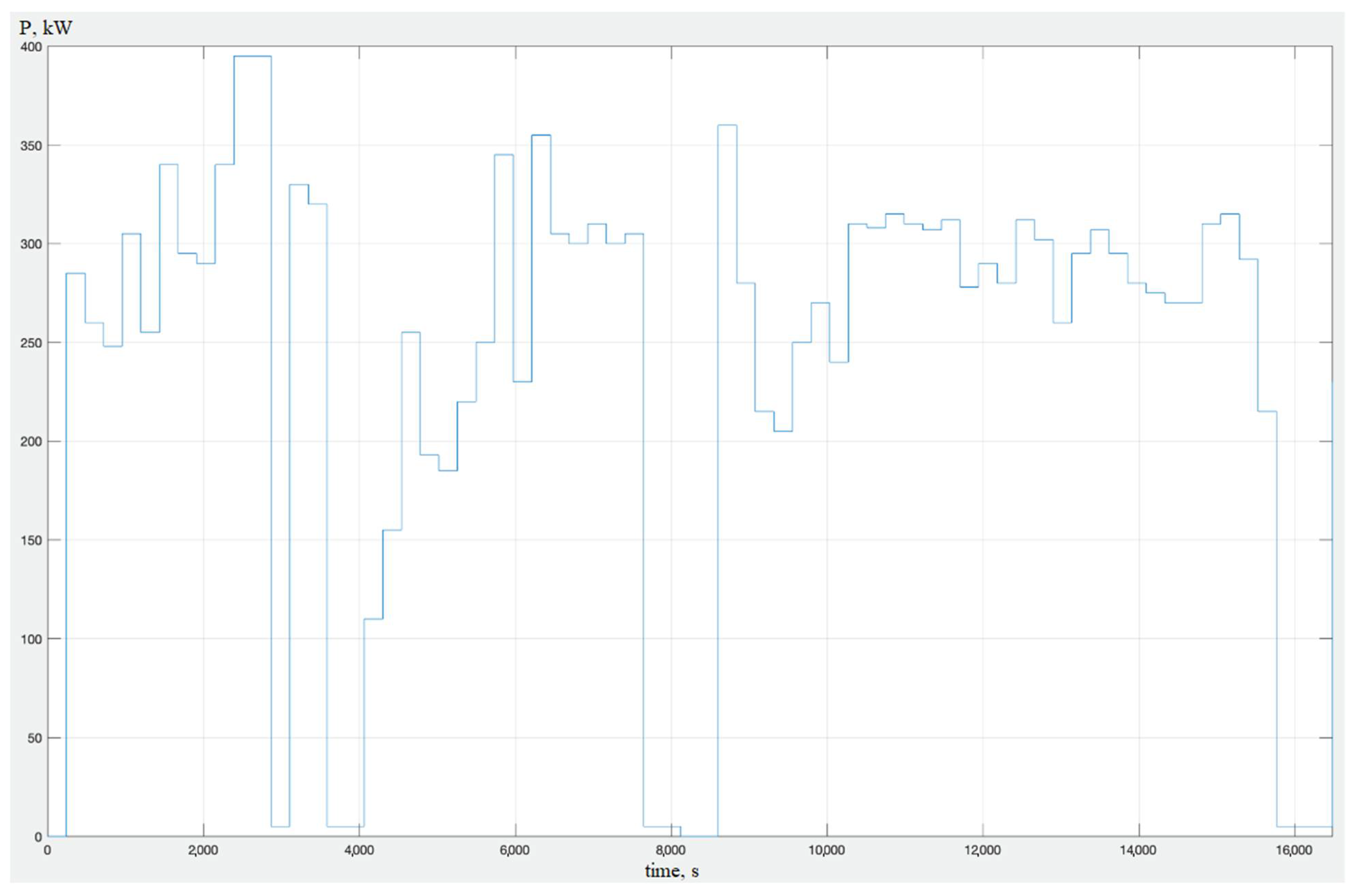
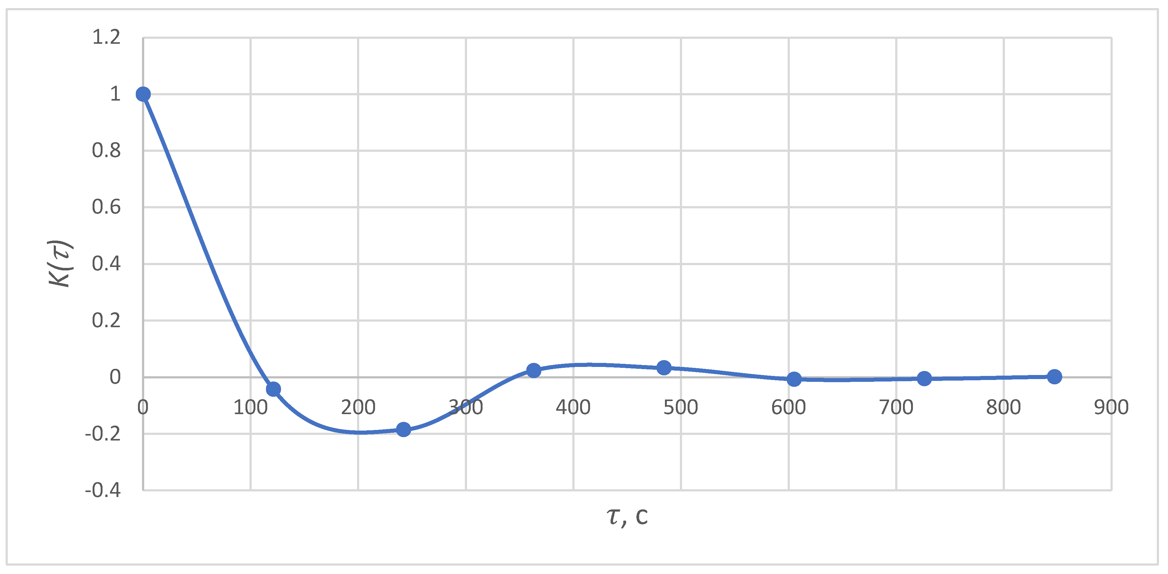
  • The given time values, namely the correlation time ( T C ), the sampling interval ( Δ t ) , and the recording time ( T r ) (Table 7), were determined according to the initial load curve (Figure 1 and Figure 2). Then, using the MATLAB software package, the experimental NCF was calculated.
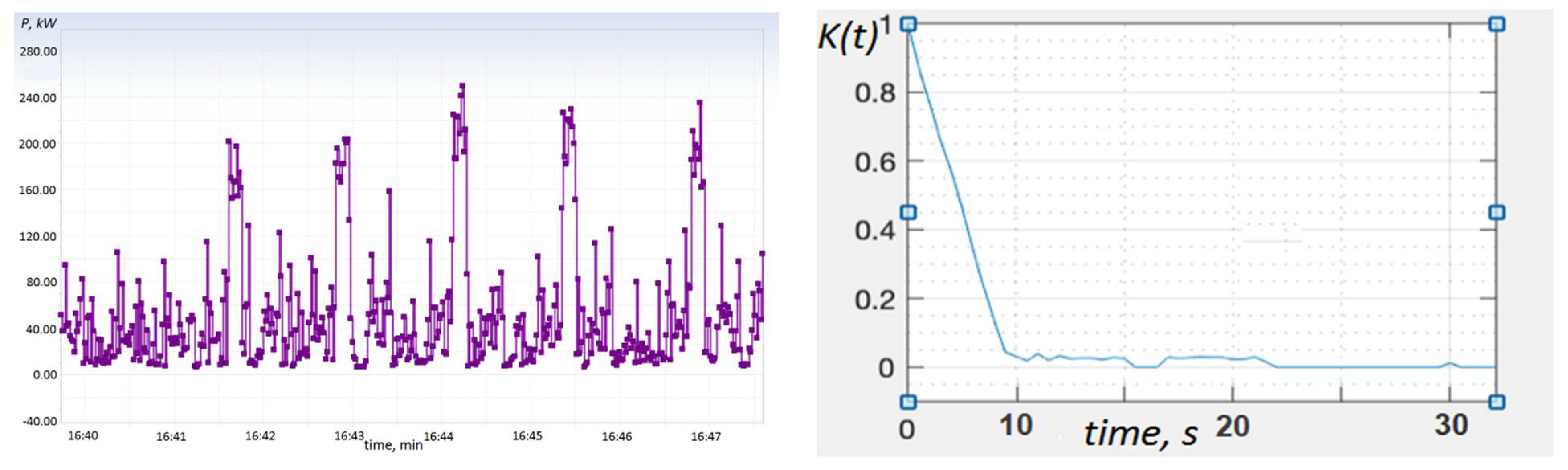
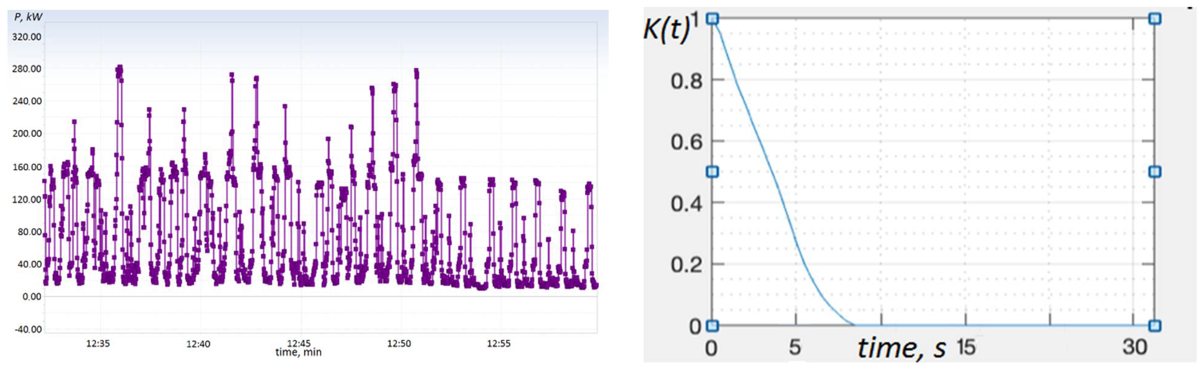
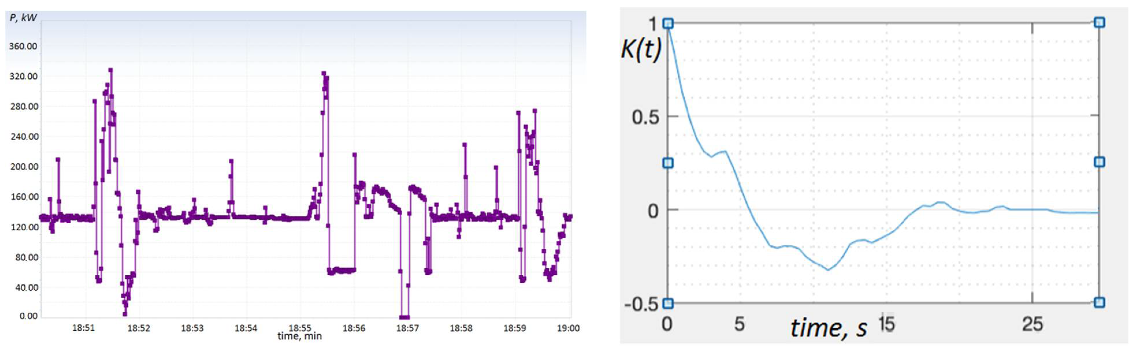
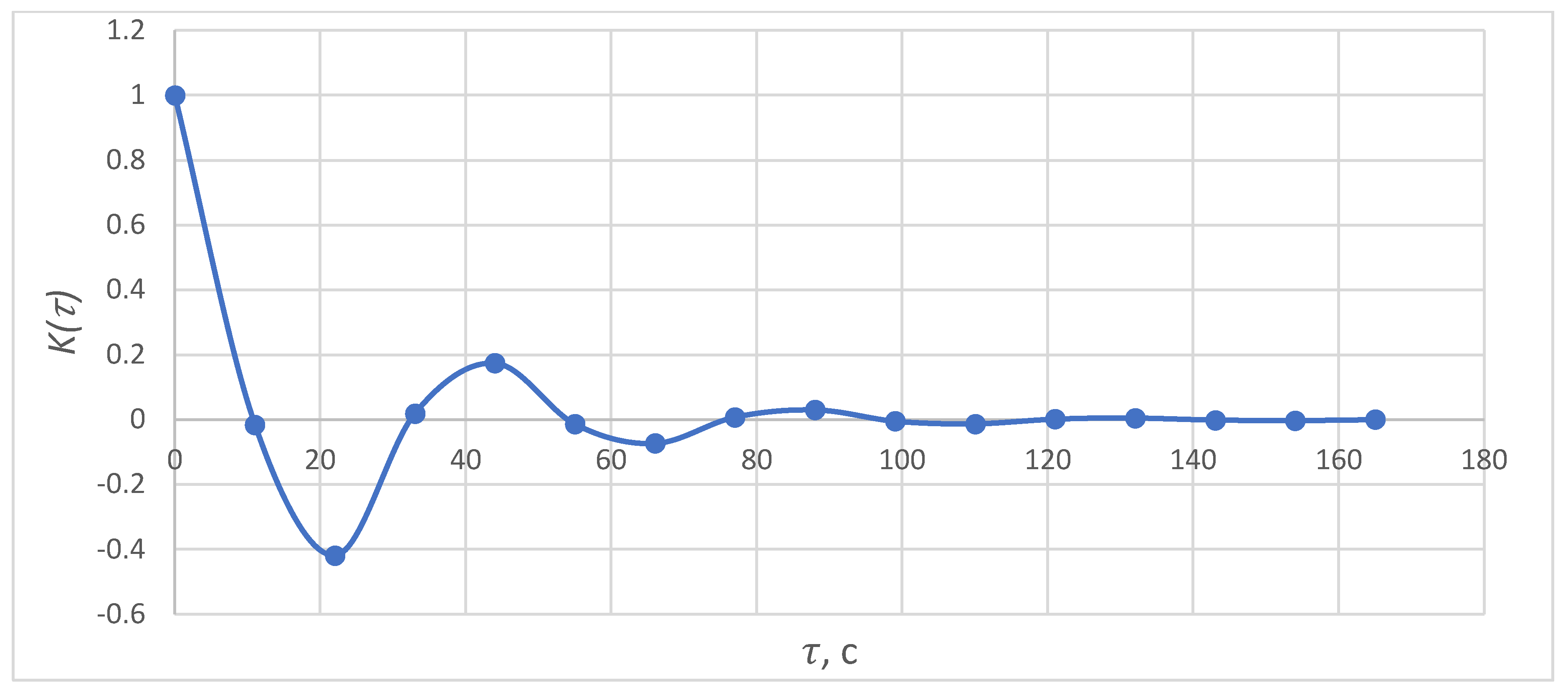
  • Using the least-squares method, we determined the parameters of a theoretical NCF, as shown in Table 8, and identified its type (Figure 3 and Figure 4).
The conducted studies showed that general-purpose industrial electric drives belong to the same type of NCF with and without the use of a variable-frequency drive, although the difference in the NCF parameters determines the calculated values of the entire power supply system. As a result, there is a need to supplement the new information database.
An additional series of loads were also studied, and the NCF and parameters were determined (Figure 5, Figure 6, Figure 7 and Figure 8 and Table 9).

4. Group Load Curve Forecasting Using a Probabilistic Calculation Method

The above operations are also valid for group curves; however, due to the variations in PSS by structure and functionality, it is necessary to perform electrical load curve forecasting by summing individual curves in order to obtain equivalent parameters of the NCF [13]. To do this, at the level of the group curves, it is necessary to use the following analytical expression:
K ( τ ) = D P e x p ( α e | τ | ) ;
where DP is the variance of the active load curve, and α э is the equivalent factor characterizing the attenuation of the correlation between the ordinates of the summed ELCs [27].
The group load curve P( t ), which is formed according to the individual curves, p ( t ), gives the following definitions for α e :
α e = D P i = 1 m D P i α i + i = 1 l D P i α i α i 2 + ω 0 i 2 + i = 1 r 2 D P i α i α i 2 + ω 0 i 2 ;
In the formula, the numbers of curves with NCF types 1, 2, 3, and 4, respectively, are taken for m ,   l ,   and   r .
Taking into account the differences in the type and parameters of the NCF for individual consumers, in Formula (6), we determine the variance of D P θ   θ peaks and θ valleys of the ELCs in the averaging interval θ :
D P θ = 2 D P ( α e θ ) 2 [ e x p ( α e θ ) + α e θ 1 ] ;

Methodology for Calculating Load Estimation Parameters

The characteristics of electrical load curves, such as θ peaks and θ valleys, make it possible to determine the following main parameters:
-
Determination of the conductor section according to the condition of heating and economic density;
-
Determination of minimum and maximum power losses;
-
Determination of voltage deviation.
The expression for determining the definition of θ peaks is as follows:
P p θ = P a v + β 1 D P θ   ;
and for θ valleys, it is as follows:
P v θ = P a v + β 2 D P θ   ;
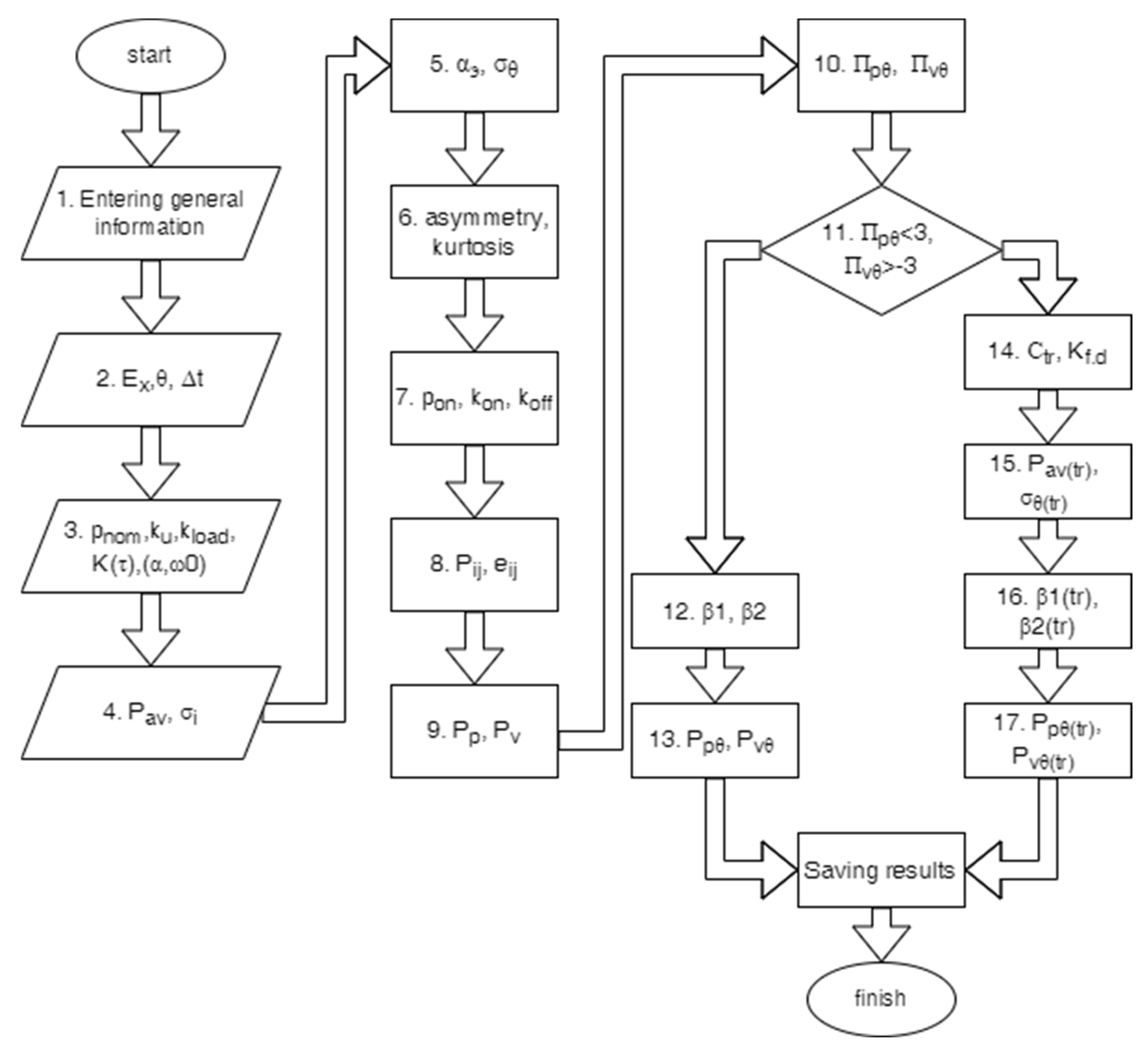
Similar to other methods of calculation of electrical loads, the HS method has its own clear sequence of actions that must be performed to obtain a result, so the task is to simplify as much as possible and create an algorithm that would not require using other sources to search information. It makes the database for the individual consumers important. Such an algorithm was developed and is presented in Figure 9.
Following each block of the algorithm, it is necessary to consider what actions take place in the system:
1.
It is necessary to indicate complete information on the design object, as well as information on the designer performing the calculation;
2.
The value corresponding to the boundary probability (Ex), the required intervals of averaging ( θ ), and discretization (Δt);
3.
Using the dataset, select the necessary equipment from the list, with the specified characteristics. Next, a group of consumers is formed, and the calculation is carried out according to the group schedule;
4.
There is a calculation of the average active and reactive power, according to the following formulas:
P a v = i = 0 m p n o m i k u i ;
Q a v = i = 0 m p n o m i k u i t g φ ;
Moreover, the calculation of the standard deviation of the active load curve is as follows:
σ i = i = 1 m p 2 n o m i k u i ( k l o a d i k u i )   ;
5.
From this block, the transition to the group graph is implemented through an equivalent correlation function, and for this, as described above, it is necessary to determine the parameter α э of the active load according to the following formula:
α э = D P i = 1 m D P i α i + i = 1 l D P i α i α i 2 + ω 0 i 2 + i = 1 r 2 D P i α i α i 2 + ω 0 i 2   ;
Moreover, the variance of the load group graph is calculated as follows:
D P θ = 2 D P ( α э θ ) 2 [ e x p ( α э θ ) + α э θ 1 ] ;
6.
In block 6, the coefficients of asymmetry (skewness) s k and kurtosis ( k ) are calculated, and for cases when the values of these coefficients are not equal to zero, it is necessary to use a law other than normal, for example, the Gram–Charlier type A distribution law [16]:
s k = i = 1 m p 3 n o m i k u i ( k l o a d i k u i ) ( k l o a d i 2 k u i ) σ 3 ;
k = i = 1 m p 4 n o m i k u i ( k l o a d i k u i ) [ ( k l o a d i k u i ) ( k l o a d i 2 k u i ) + k 2 u i ] + 6 i < j σ i 2 σ j 2 σ 4 3 ;
7.
From block 7, we see that the algorithm for estimating the characteristics of group curve begins, taking into account the limitations of the limits of its change; thus, it is necessary to calculate additional characteristics for individual consumers, such as the following:
the value of the average power during switch-on time t o n ,
p o n = p n o m k l o a d ;
the value of the switch-on factor as the probability of the “on” mode,
k o n = k u k l o a d ;  
and the value of the switch-off factor as the probability of the “off” mode,
k o f f = 1 k o n .
8.
Searching through the combinations of the ith modes “on” and the jth modes “off”, we see that the possible ordinates for the ELCs are determined, and using the theorem of the product of probabilities, we obtain the probability of a single combination [28,29]:
e i j = i = 0 m k o n i j = 0 n m k o f f j ;
In Formula (11), the value m denotes the consumers operating in the “on” mode and with the corresponding k o n i , while the value n-m denotes the consumers operating in the “off” mode and with the corresponding k o f f j .
The electrical load values correspond to the probabilities, e i j :
P i j = i = 0 m p o n i ;
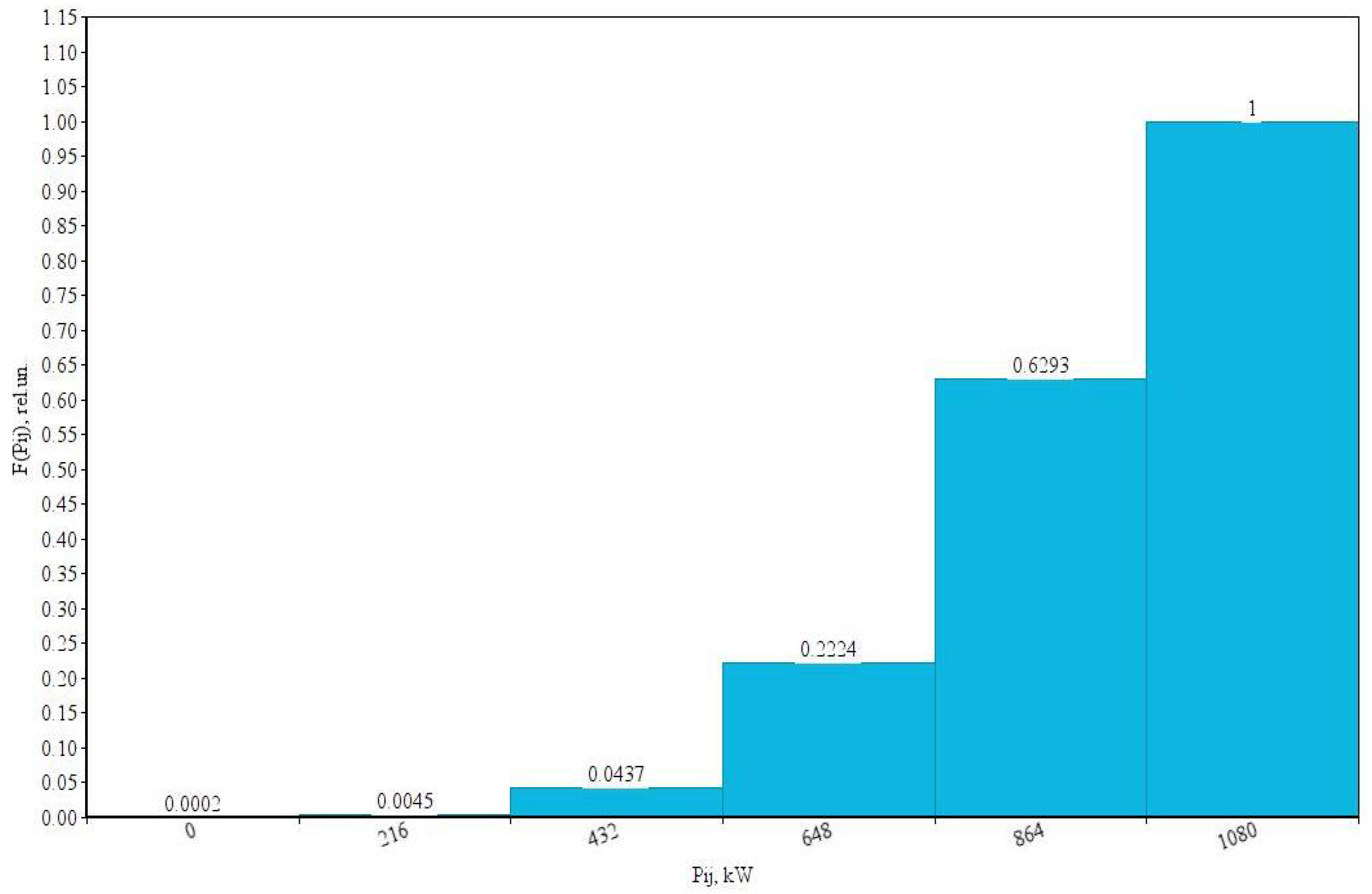
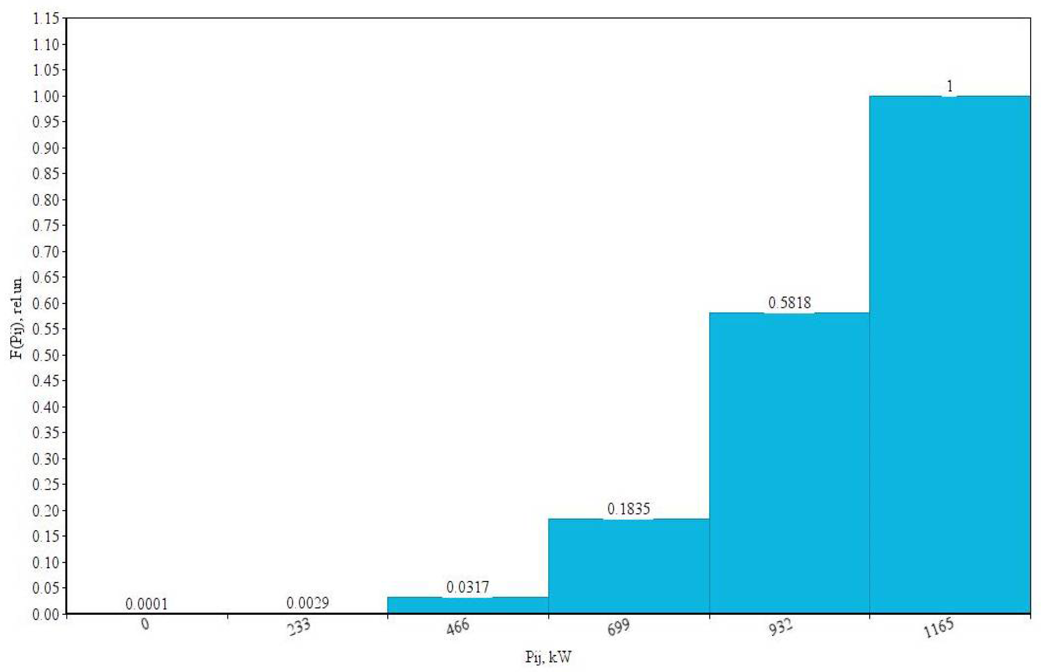
If the same load arises as a result of different combinations of different options for the work of consumers, there is a general probability of the occurrence of a given load arising in a given complex situation of probabilities [30]. As a result, a statistical series is formed, according to which the step function of the probability distribution of the ordinates ELC F(P) is constructed. To determine the actual lower (valley) P v and upper (peak) P p values of the limits of variation of the ordinates of the ELC, the principle of practical confidence of the theory of probabilities is used [17]. According to this principle, practically impossible values of electrical loads are excluded from the obtained possible range of electrical load values from 0 to i = 1 m p o n i , which have a lower probability than the boundary probability, Ex = 0.05.
9.
Furthermore, according to Expressions (8) and (9) above, θ peaks and θ valleys are determined.
10.
From the theory of electrical loads, it is known that the calculated values of the load curve are limited by the upper limit, which is obtained by summing all individual consumers, as well as the lower limit, which corresponds to the complete absence of load. In real industrial conditions, the upper design limits are always higher than the real maximum values, while for the lower limit, the load is usually greater than zero. Consequently, due to the disagreement between the real and theoretical limits, an error occurs in the calculations of the peaks, P p θ , and the valleys, P p B θ . For this, in addition to the normal distribution law, it is also necessary to consider the “truncated” normal distribution law, and for this, it is necessary to determine the values of the normalized upper and lower limits:
Π p θ = ( P p P a v ) σ θ ;
Π v θ = ( P v P a v ) σ θ ;
11.
Furthermore, according to the results obtained in block 10, the values are checked according to the normalized limits according to the following conditions:
-
For Π p θ   >   3   and   Π v θ   <   3 , the calculation is performed for blocks 12 and 13 by using the normal distribution law;
-
For Π p θ   <   3   and   Π v θ   >   3 , the calculation is performed in blocks 14–17, using the “truncated” normal distribution law.
12.
Calculation of statistical coefficients and calculation of power peaks and valleys.
13.
The use of the “truncated” normal distribution law is possible by introducing the truncation coefficient, C t r , into probabilistic models and form factor, K f . d θ [16,31]:
C t r = + f ( P θ ) d P θ P v θ P p θ f t r ( P θ ) d P θ ;
After a series of mathematical transformations, the truncation coefficient, C t r , expressed through the normalized function, Φ * , of the normal distribution law, is defined by the following formula [32,33]:
C t r = [ Φ * ( Π p θ ) Φ * ( Π v θ ) ] ;
K f . d θ = 1 + D P θ P a v 2 ;
14.
Furthermore, taking into account the limits on the maximum and minimum values, the value of the average power and the standard deviation are determined as follows:
P a v ( t r ) = P a v ± σ θ C t r = [ φ * ( Π p θ ) φ * ( Π v θ ) ] ;
where φ * ( П p , v θ ) is the density of the standard normal distribution [34]. The standard deviation of the load is as follows:
σ θ ( t r ) = σ θ { 1 + C t r [ Π v θ φ * ( Π v θ ) Π p θ φ * ( Π p θ ) ] C t r 2 [ φ * ( Π v θ ) φ * ( Π p θ ) ] 2 } ;
15.
In block 16, the statistical coefficients β 1 ( t r ) and β 2 ( t r ) are as follows:
1 E x = C t r 2 π σ θ P v θ P p θ ( t r ) exp ( ( P θ P a v ) 2 2 σ θ 2 ) d P θ ;
E x = C t r 2 π σ θ P v θ P p θ ( t r ) exp ( ( P θ P a v ) 2 2 σ θ 2 ) d P θ ;
16.
Next θ —peaks P p ( t r ) , and θ —valleys P v ( t r ) are calculated through the average power and statistical coefficients, taking into account truncation:
P p θ ( t r ) = P a v ( t r ) + σ θ ( t r ) β 1 ( t r ) ;
P v θ ( t r ) = P a v ( t r ) σ θ ( t r ) β 2 ( t r ) ;

5. Discussion

Below are the results of the studies carried out according to the above-described methodology on the example of group curves of the load of conveyor units. A feature of this method is the determination of the actual consumption of active power, both with and without the use of variable-frequency drives. For this purpose, measurements of power consumption were taken at the facility during one of the most loaded shifts, with a duration of T r = 8 h and with a sampling interval Δ t a = 1   min . [17,32] Such parameters allow for sufficient reliability when assessing the range of voltage deviations in electrical networks at the lower stages of the PSS (Table 10).
The parameters of the NCF and the recalculated utilization factor ( k u ) were defined by other authors earlier, with a detailed overview of the scientific research [4,26].
Furthermore, using the calculation formulae, we determined the probabilistic characteristics of the group ELC (Table 11).
Furthermore, it is necessary to calculate the switch-on and -off factors according to (9) and (10), respectively, and also to calculate power consumption during the switch-on time according to (8). The data are summarized in Table 12.
Using (11) and (12), we can determine the probabilities, e i j , of the occurrence of an electric load ( P i j ), according to which we can build two static series, which are summarized in Table 13 and Table 14 and shown in graphical form in Figure 10 and Figure 11 for a group curve, both without the use of and with the use of frequency control, respectively.
Having analyzed the obtained static series of the probability distribution of the group curve without using frequency control, we can now select the lowest P v = 466   kW and the highest P p = 1165   kW , and then with the use of frequency control, the lowest P v = 432   kW and the highest P p = 1080   kW .
Furthermore, using the specified averaging interval equal to 1 min, the upper and lower limits of change of θ-ordinates are calculated according to (13) and (14). The calculation results for the normalized limits are summarized in Table 15.
The results of intermediate studies proved the significant limitations in magnitude; therefore, further assessment of the calculated values of the peaks and valleys of conveyor units in order to compare the two distribution laws described above must be carried out by using these limitations, taking into account the truncation factor, C t r [32,35]. Using Equations (24)–(32), we obtained the values which are summarized in Table 16.
The resulting errors in the assessment of the calculated values of peaks and valleys relative to the two laws of distribution of the normal law and the truncated normal law are calculated by using the following expression [8]:
δ p , v θ = | P p , v θ ( t r ) P p , v θ | P p , v θ ( t r ) 100 % ;
The error is no more than 6%, which does not go beyond the limits of permissible values of ± 10 % [36]; however, the use of a variable frequency drive is not considered, where the error is as follows:
δ P v θ = 44 %
δ P p θ = 38 %
This clearly goes beyond the limits of permissible values, causing us to consider a variable frequency drive as a separate load that has its own parameters.
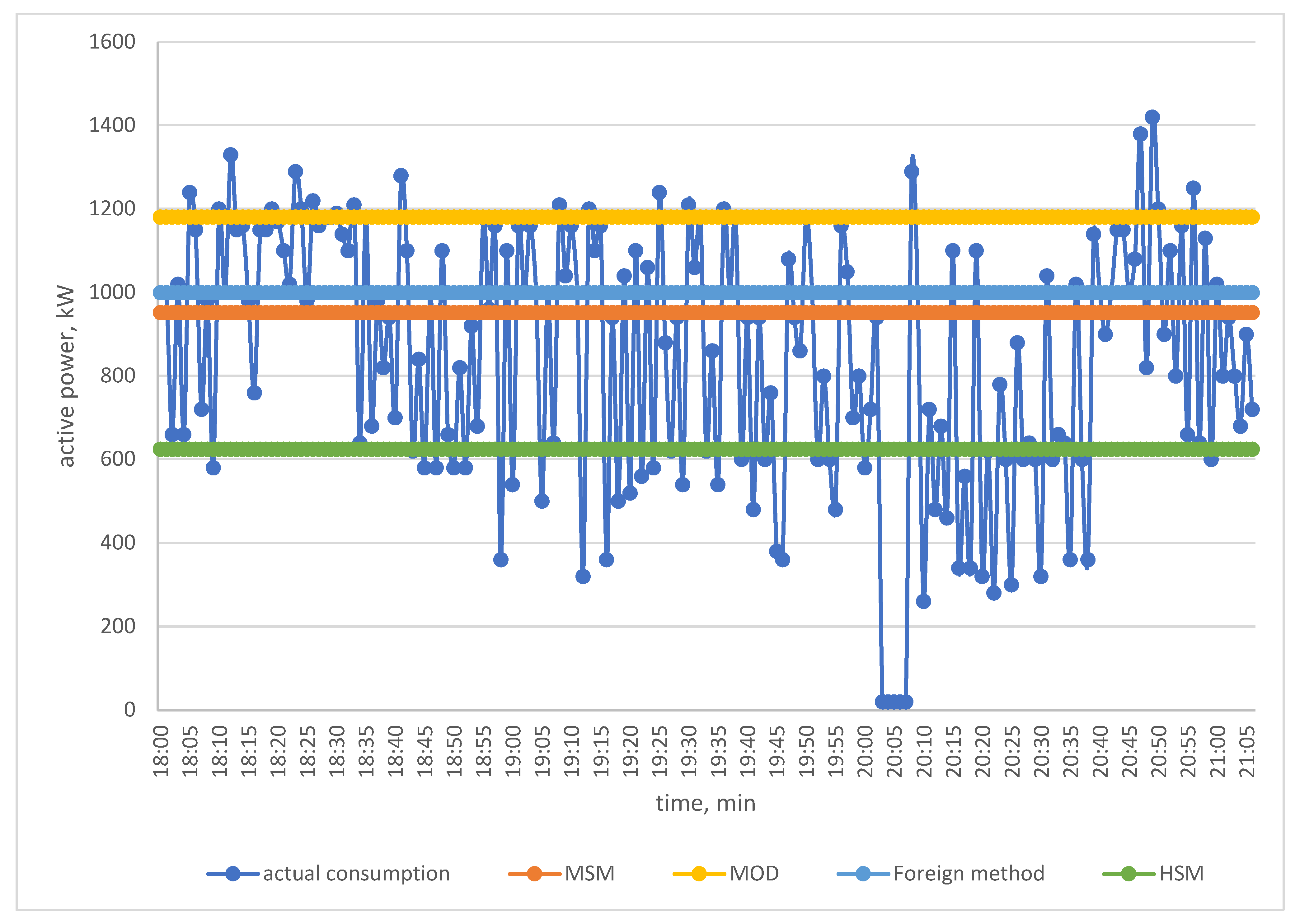
Foreign methods, as well as the method of ordered diagrams and the modified statistical method (Table 17), do not allow the effects from using a variable-frequency drive to be assessed, and all attempts to do this by adjusting the utilization factor failed [37,38]. Figure 12 shows the values of the average calculated loads defined by using various methods.

6. Conclusions

In this study, a method was developed for determining the design calculated electrical loads of mining enterprises that also takes into account the dynamic characteristics of load changes, such as peaks and troughs, surges and load dips, and load fluctuations, which will solve the problems of performing electrical load calculations with a higher confidence probability. These load characteristics were not taken into account in previous studies. This has been shown to have a significant impact on the resulting design power. As a result of increasing the reliability of determining the calculated values of electrical loads, it became possible to make the right choice of power and switching electrical equipment for distribution and protection, which will lead to a reduction in material costs.
The experimental and theoretical studies were carried out personally at the mining facilities, while the gathering of initial data took about 2 years. The initial obtained data made it possible to expand the information base for various consumers, thereby increasing interest in using this calculation method, which ultimately will allow us to design high-quality power supply systems.
The technique proposed in this article can be extended in several aspects by including the technologies of neural networks and machine learning in the calculation.

Author Contributions

D.A.U. defined the general concept for the work and research and arranged for conducting experimental research at enterprises. K.A.K. collected initial data at the mining and processing enterprises, analyzed existing methods used for calculating electrical loads, determined the NCF for individual and group load schedules, and determined dynamic characteristics of the electrical loads graphs. All authors have read and agreed to the published version of the manuscript.

Funding

This research received no external funding.

Institutional Review Board Statement

Not applicable.

Informed Consent Statement

Inapplicable.

Data Availability Statement

Data available upon request, due to restrictions, e.g., privacy or ethical restrictions. The data presented in this study are available upon request from the corresponding author. The data are not publicly available (due to the fact that row data were obtained from industrial facilities).

Conflicts of Interest

The authors declare no conflict of interest.

Nomenclature

p ( t )Individual curves(kW)
P( t )Group load curve(kW)
P av Average power(kW)
P h Heating power(kW)
T c Correlation time(s)
Δ t Sampling interval(s)
T r Recording time(s)
P p Peak of the actual values of the ELC(kW)
P v Valley of the actual values of the ELC(kW)
p o n Average power during switch-on time(kW)
p n o m Rated power(kW)
P i j Electrical load values corresponding to the probabilities e i j (kW)
D p Variance of an individual electrical load curve(kW2)
DPVariance of group electrical load curve(kW2)
Θ Averaging interval(min.)
DP θ Variance of group electrical load curve on the averaging interval θ (kW2)
σ θ Standard deviation of the load on the averaging interval θ (kW)
α Parameter characterizes the attenuation of correlations between the ordinates of the initial ELC(1/s)
ω 0 The natural frequency of oscillations of the CF, due to the repeatability of technological operations(1/s)
α э Equivalent factor characterizing the attenuation of correlation between the ordinates of the summed ELCs(1/s)
e i j Probability of a single combination(rel.un.)
F(P)Probability distribution function of the ELC(rel.un.)
ExBoundary probability(1)
П p θ Normalized upper limit(rel.un.)
П v θ Normalized lower limit(rel.un.)
β 1 , 2 Statistical coefficient(rel.un.)
Φ * Normalized function of the normal distribution law(rel.un.)
φ * Density of the normal distribution law(rel.un.)
δ p , v θ Resulting errors in the assessment of the calculated values of peaks and valleys(%)
k u Utilization factor
k d Demand factor
k M Peak coincidence factor
K ( τ ) Normalized correlation function
k l o a d Load factor
k o n Switch-on factor
k o f f Switch-off factor
C tr Truncation coefficient

Abbreviations

SMStatistical method
MODMethod of ordered diagrams
MSMModified statistical method
HSMHierarchical–structural method
VFDVariable-frequency drive
PSSPower supply system
CFCorrelation functions
NCFNormalized correlation function
ELCElectrical load curve

References

  1. Uryadnikov, N.V. Electricity Consumption in the Russian Federation. Available online: https://www.fedstat.ru/indicator/43277 (accessed on 6 October 2021).
  2. Kozyaruk, A.E.; Vasiliev, B.Y. Methods and means for increasing the energy efficiency of machines and technologies with asynchronous electric drives. Bull. South Ural. State Univ. 2014, 1, 47–53. [Google Scholar]
  3. Khomiakov, K.A.; Belyakov, S.A. The use of RIVS-manufacture energy-saving electric motors in min-ing and processing facilities. J. Min. Univ. 2016, 11, 29–32. [Google Scholar]
  4. Khan, I.; Jemai, J.; Lim, H.; Sarkar, B. Effect of Electrical Energy on the Manufacturing Setup Cost Reduction, Transportation Discounts, and Process Quality Improvement in a Two-Echelon Supply Chain Management under a Service-Level Constraint. Energies 2019, 12, 3733. [Google Scholar] [CrossRef] [Green Version]
  5. Mahapatra, A.S.; Soni, H.N.; Mahapatra, M.S.; Sarkar, B.; Majumder, S. A Continuous Review Production-Inventory System with a Variable Preparation Time in a Fuzzy Random Environment. Mathematics 2021, 9, 747. [Google Scholar] [CrossRef]
  6. Sinchuk, O.N.; Guzov, E.S. Improvement of methods for calculating electrical loads in the design of power supply systems at iron ore enterprises. Bull. KrNU Mikhail Ostrogradsky 2013, 1, 28–32. [Google Scholar]
  7. Zhokhov, B.D. Analysis of the causes of the overestimation of calculated loads and their possible correction. Ind. Power Eng. 1989, 7, 7–9. [Google Scholar]
  8. Khomiakov, K.A.; Ustinov, D.A. Improving the accuracy of calculation of electrical loads for industrial enterprises. J. Phys. Conf. Ser. 2019, 1333, 062009. [Google Scholar] [CrossRef]
  9. Ali Hassan Electrical Load Estimation Course. Available online: http://www.electrical-knowhow.com/2012/12/electrical-pdf-courses.html (accessed on 1 November 2012).
  10. Krotkov, E.A.; Stepanov, V.P. Assessment of errors of calculated electric power losses in industrial electrical networks. Energy Sav. 2000, 3, 47–79. [Google Scholar]
  11. Kampelis, N.; Tsekeri, E.; Kolokotsa, D.; Kalaitzakis, K.; Isidori, D.; Cristalli, C. Development of Demand Response Energy Management Optimization at Building and District Levels Using Genetic Algorithm and Artificial Neural Network Modelling Power Predictions. Energies 2018, 11, 3012. [Google Scholar] [CrossRef] [Green Version]
  12. Stepanov, V.P.; Krotkov, E.A. Theoretical substantiotion of the sampling interval for calculation the carrelation functions of electric load graphs Power engineering control quality and energy efficiency. In Proceedings of the Russian Scientific and Technical Conference “Energy: Management, Quality and Efficiency of Energy Resources Use”, Blagoveshchensk, Russia, 14–16 October 1998; pp. 70–74. [Google Scholar]
  13. Ustinov, D.A.; Khomiakov, K.A. Comprehensive assessment of factors determining electricity load curves concerning enterprises of mineral resource sector. J. Phisics Conf. Ser. 2020, 1753, 012061. [Google Scholar] [CrossRef]
  14. Abramovich, B.N. Uninterruptible Power Supply System for Mining Industry Enterprises. J. Min. Inst. 2018, 229, 31–40. [Google Scholar]
  15. Saidur, R. A review on electrical motors energy use and energy savings. In Renewable and Sustainable Energy Reviews. Elsivier: Amsterdam, The Netherlands, 2010; Volume 14, pp. 877–898. ISSN 1364-0321. [Google Scholar] [CrossRef]
  16. Khomiakov, K.A.; Ustinov, D.A. Adjusting the method for calculating electrical loads of mining enterprises. J. Eng. Sci. Technol. SPbPU Nat. Eng. Sci. 2019, 1, 71–78. [Google Scholar]
  17. Stepanov, V.P.; Krotkov, E.A.; Vedernikov, A.S.; Gudkov, A.V.; Idiatullin, R.F. Reasons for overestimating the calculated values of peaks and valleys of electrical load curves of machine-building plants. Ind. Power Eng. 2006, 1, 27–30. [Google Scholar]
  18. Zhezhelenko, I.V.; Stepanov, V.P.; Gudkov, A.V.; Iduatulin, R.F. Influence of possible ordinates of electrical load curves on calculated values of peaks and valleys of load. Energ. CIS High. Educ. Inst. Power Eng. Assoc. 2006, 2, 5–12. [Google Scholar]
  19. Nikolaev, N.I.; Shipulin, A.V.; Kupavykh, K.S. Improving the energy efficiency of well development. J. Eng. Sci. Technol. SPbPU Nat. Eng. Sci. 2015, 2, 48–57. [Google Scholar]
  20. Ullah, K.R.; Thirugnanasambandam, M.; Saidur, R.; Rahman, K.A.; Kayser, M.R. Analysis of Energy Use and Energy Savings: A Case Study of a Condiment Industry in India. Energies 2021, 14, 4798. [Google Scholar] [CrossRef]
  21. Seppälä, A. Load Research and Load Estimation in Electricity Distribution; VTT Publications 289; Technical Research Centre of Finland: Espoo, Finland, 1996; pp. 1–118. [Google Scholar]
  22. Abramovich, B.N.; Sychev, Y.A. Problems of ensuring energy security for enterprises from the mineral resources sector. J. Min. Inst. 2016, 217, 132–139. [Google Scholar]
  23. Evangelopoulos, V.; Karafotis, P.; Georgilakis, P. Probabilistic Spatial Load Forecasting Based on Hierarchical Trending Method. Energies 2020, 13, 4643. [Google Scholar] [CrossRef]
  24. Strokov, A.Y.; Belyaev, A.N. Improving the dynamic stability of stand-alone energy grids based on the data from monitoring of transient processes. J. Eng. Sci. Technol. SPbPU Nat. Eng. Sci. 2015, 1, 48–58. [Google Scholar]
  25. Anishchenko, V.A.; Pisaruk, T.V. Monitoring the reliability of measurements of load at industrial enterprises on the basis of the analysis of the dynamics of load alterations. Energ. CIS High. Educ. Inst. Power Eng. Assoc. 2020, 63, 393–410. [Google Scholar]
  26. Shevyrev, Y.V.; Datskovsky, L.K.; Boguslavsky, I.Z. Selection of the type of electric drive for large-volume mills. J. Min. Univ. 2020, 5, 53–62. [Google Scholar]
  27. Anishchenko, V.A.; Pisaruk, T.V. Monitoring the reliability of measurements in energy grids according to the first increment and on the basis of extrapolating filters. Energ. CIS High. Educ. Inst. Power Eng. Assoc. 2018, 61, 423–431. [Google Scholar]
  28. Galkin, V.I. Extension of application range of tubular belt conveyors owing to constructive inno-vative solutions. J. Min. Univ. 2020, 5, 52–56. [Google Scholar]
  29. Keka, I.; Betim, C.; Neki, F. Effect of parallelism in calculating the execution time during forecasting electrical load. JNTS 2017, 44, 169–180. [Google Scholar]
  30. Khuntia, S.R.; Ruenda, J.L.; Van der Meijden, M.A. Long-term electricity load forecasting considering volatility using multiplicative error model. Energies 2018, 11, 3308. [Google Scholar] [CrossRef] [Green Version]
  31. Chen, P. Stochastic Modeling and Analysis of Power System with Renewable Generation. Ph.D. Thesis, Aalborg University, Aalborg, Denmark, 2010; pp. 1–216. [Google Scholar]
  32. Shklyarskiy, Y.; Hanzelka, Z.; Skamyin, A. Experimental Study of Harmonic Influence on Electrical Energy Metering. Energies 2020, 13, 5536. [Google Scholar] [CrossRef]
  33. Shklyarskiy, Y.; Skamyin, A.; Vladimirov, I.; Gazizov, F. Distortion Load Identification Based on the Application of Compensating Devices. Energies 2020, 13, 1430. [Google Scholar] [CrossRef] [Green Version]
  34. Sychev, Y.; Abramovich, B.; Prokhorova, V. The assessment of the shunt active filter efficiency under varied power supply source and load parameters. Int. J. Electr. Comput. Eng. 2020, 10, 5621–5630. [Google Scholar]
  35. Zagrivniy, E.A.; Poddubniy, D.A.; Kovalchuk, M.S. Noncontact speed sensor for maintaining the autoresonant operating mode of the oscillating electric motor drive. In Proceedings of the 2019 IEEE Conference of Russian Young Researchers in Electrical and Electronic Engineering, Saint Petersburg, Russia, 28–31 January 2019; pp. 740–743. [Google Scholar]
  36. Kovalchuk, M.S.; Zagrivniy, E.A.; Poddubniy, D.A. Simulation Model of a Dynamically Coun-terbalanced Drilling String with a Sensorless Control System for Controlling an Autoresonant AC Electric Drive. In Proceedings of the IEEE Conference of Russian Young Researchers in Electrical and Electronic Engineering, Saint Petersburg, Russia, 27–30 January 2020. [Google Scholar]
  37. Baburin, S.V.; Zyrin, V.O.; Kovalchuk, M.S. Dependence of power supply systems reliability on the type of redundancy. In Proceedings of the IOP Conference Series: Materials Science and Engineering, Saint Petersburg, Russia, 23–24 May 2019; Volume 643. [Google Scholar]
  38. Belsky, A.A.; Skamyin, A.N.; Vasilkov, O.S. The Use of Hybrid Energy Storage Devices for Balancing the Electricity Load Profile of Enterprises. Energ. CIS High. Educ. Inst. Power Eng. Assoc. 2020, 63, 212–222. [Google Scholar] [CrossRef]
Figure 1. Fragment of the curve of active power consumption without a VFD.
Electricity 03 00010 g001
Figure 2. Fragment of the curve of active power consumption with a VFD.
Electricity 03 00010 g002
Figure 3. Theoretical NCF curve without a VFD.
Electricity 03 00010 g003
Figure 4. Theoretical NCF curve with a VFD.
Electricity 03 00010 g004
Figure 5. Fragment of the curve of active power consumption hydrocyclone feed pump with a VFD and his NCF.
Electricity 03 00010 g005
Figure 6. Fragment of the curve of active power consumption crushers with a VFD and his NCF.
Electricity 03 00010 g006
Figure 7. Fragment of the curve of active power consumption overhead crane with a VFD and his NCF.
Electricity 03 00010 g007
Figure 8. Fragment of the curve of active power consumption pneumatic–mechanical flotation tank cells without a VFD and his NCF.
Electricity 03 00010 g008
Figure 9. Algorithm for calculating the parameters of electrical load curves.
Electricity 03 00010 g009
Figure 10. Step function of the probability distribution of the ordinates of the initial group ELC with the use of frequency control.
Electricity 03 00010 g010
Figure 11. Step function of the probability distribution of the ordinates of the initial group ELC with the use of frequency control.
Electricity 03 00010 g011
Figure 12. Actual values for the electrical load curves and the calculated values for the average load power.
Electricity 03 00010 g012
Table 1. Contributions of authors.
Author(s)Probabilistic MethodLarge Accumulated Database Containing the Source DataSimplicity of Performing Engineering CalculationsCorrelation between OrdinatesAccount the Modern Means to Improve Energy Efficiency
Sinchuk, O.N. Guzov, E.S. [6]
Zhokhov, B.D. [7]
Ali Hassan [9]
Stepanov, V.P [17]
This paper√ √√ √√ √√ √√ √
Table 2. Average values of consumed active power ( P av ), in kW, for the test period.
Consumer TypeWithout a VFDWith a VFD
Conveyor174.8138.9
Hydrocyclone feed pump44.330.3
Blower217.5159.5
Overhead crane14.09.0
Table 3. Utilization factors.
Consumer Type k u .   Reference   Value   k u   Actual   Value   without   VFD k u   Actual   Value   with   VFD
Conveyor0.750.700.5
Hydrocyclone feed pump0.800.780.55
Blower0.750.720.56
Overhead crane0.450.400.25
Table 4. Advantages and disadvantages of existing load calculation methods used for calculating electrical loads.
Load Calculation Method Disadvantages Advantages
  • Method of ordered diagrams;
  • Statistical method
  • Modified statistical method.
-
The use of approximate formulae according to which the thirty-minute maximum load is recalculated;
-
Correlation and inter-correlation between ordinates are not taken into account, both at the level of individual and group electrical load curves of an electric drive;
-
The average load is assessed based on the upper limits of the probabilistic values;
-
Overestimation of the average value of the load factors to assess the calculated heating load;
-
Discrepancy between the design technological modes and the actual operating modes.
-
Large accumulated database containing the source data;
-
Simplicity of performing engineering calculations.
Table 5. Database with additional characteristics.
Effective number of power consumers n
Rated power p n o m
Utilization factor k u
Power factor t g φ
Normalized correlation function K ( τ )
Parameter characterizes the attenuation of correlations between the ordinates of the initial ELC α
The natural frequency of oscillations of the CF, due to the repeatability of technological operations ω 0
Table 6. Approximate average power values.
Without a VFD With a VFD
P av = 175   kW P av = 139   kW
Table 7. The time values.
Correlation   Time ,   T c Sampling   Interval ,   Δ t Recording   Time ,   T r
Without a VFD With a VFDWithout a VFDWith a VFDWithout a VFDWith a VFD
69.5   s 14.5   s 0.695 s 0.145   s 5560   s 1160   s
Table 8. Theoretical NCFs.
Theoretical NCF without a VFDTheoretical NCF with a VFD
K ( τ ) = e x p ( 1.723 | τ | ) cos ( 2.26 τ ) K ( τ ) = e x p ( 3.37 | τ | ) cos ( 10.23 τ )
Table 9. Parameters of the various types of NCFs, with and without the use of a frequency converter.
Electric Drive Name Without a VFDWith a VFD
Type of the NCF Parameters of the NCF Type of the NCF Parameters of the NCF
α ,   s 1 ω 0 ,   rad / s α ,   s 1 ω 0 ,   rad / s
Conveyor 21.7232.2623.3710.23
Hydrocyclone feed pump10.701.1811.953.04
Blower10.290.7310.871.08
Crushers---11.072.01
Pneumatic–mechanical flotation tank cells20.981.34---
Overhead crane 40.451.0540.92.25
Fans10.015----
Cylindrical grinding machine 20.0780.268---
Table 10. Reference information for an ED.
Without Frequency Control
Unit NameQuantity, pcs. P n o m   kW k u   k l o a d   k o n Parameters of the NCF
Type α ,   s 1 ω 0 ,   rad / s
Main conveyer 52500.70.830.84(2)1.7232.26
With frequency control
Main conveyer 52500.50.610.82(2)311
Table 11. Calculation formulae for the probabilistic characteristics of individual and group ELCs.
Characteristics of Individual ELCs Characteristics of Group ELCs
Unit Name p a v i   kW σ i   kW σ P a v   α e   σ θ = 1  
Without frequency control
Main conveyer 5ЮЗ1751711718754.69165
With frequency control
Main conveyer 5ЮЗ1252501316258.33125
Table 12. Probabilistic design characteristics for the group ELC.
Unit Name p o n kW k o n k o f f
Without frequency control
Main conveyer4660.840.16
With frequency control
Main conveyer 54320.820.18
Table 13. Static series of the probability distribution of ordinates of the initial group ELC without using frequency control.
P i j ,   kW e i j ,   rel . un . F ( P i j ) ,   rel . un .
00.00010.0001
2330.00280.0029
4660.02890.0317
6990.15170.1835
9320.39830.5818
11650.41821.0000
Table 14. Static series of the probability distribution of ordinates of the initial group ELC with the use of frequency control.
P i j ,   kW e i j ,   rel . un . F ( P i j ) ,   rel . un .
00.00020.0002
2160.00430.0045
4320.03920.0437
6480.17860.2224
8640.40690.6293
10800.37071.0000
Table 15. Calculated values of the limits of change of the ordinates.
θ ,   m i n P v ,   k W P p ,   k W P a v ,   k W σ θ ,   k W П v θ П p θ
Without frequency control
14661165875165−2.481.76
With frequency control
14321080625125−1.542.99
Table 16. Calculated values of the limits of change of ordinates, taking into account the truncation by the upper and lower limits.
θ ,
m i n
П v θ П p θ C t r k f . d θ P a v ( t r )
k W
σ θ ( t r ) ,   k W β 2 ( t r ) β 2 ( t r ) P v θ ( t r )
k W
P p θ ( t r )
k W
Without frequency control
1−2.481.761.0441.1863.5146.71.5871.7256101096
With frequency control
1−1.542.991.0731.02609110.41.7371.532440801
Table 17. Errors in determining the average value of power, P a v , with various methods using a VFD relative to the hierarchical–structural method according to the truncated normal law.
Methods for Assessing Calculated Loads P a v ,   k W δ P a v ,   %
Experimental values615-
The modified statistical method 96637
The method of ordered diagrams 118148
Foreign method 100039
Hierarchical–structural method6251,4
Publisher’s Note: MDPI stays neutral with regard to jurisdictional claims in published maps and institutional affiliations.

