Article

Classification of Nuclear Reactor Operations Using Spatial Importance and Multisensor Networks

by
Jake Tibbetts
1,
Bethany L. Goldblum
1,2,*,
Christopher Stewart
1 and
Arman Hashemizadeh
1
1
Department of Nuclear Engineering, University of California, Berkeley, CA 94720, USA
2
Nuclear Science Division, Lawrence Berkeley National Laboratory, Berkeley, CA 94720, USA
*
Author to whom correspondence should be addressed.
J. Nucl. Eng. 2022, 3(4), 243-262; https://doi.org/10.3390/jne3040014
Submission received: 5 June 2022 / Revised: 29 August 2022 / Accepted: 13 September 2022 / Published: 22 September 2022

Abstract

:
Distributed multisensor networks record multiple data streams that can be used as inputs to machine learning models designed to classify operations relevant to proliferation at nuclear reactors. The goal of this work is to demonstrate methods to assess the importance of each node (a single multisensor) and region (a group of proximate multisensors) to machine learning model performance in a reactor monitoring scenario. This, in turn, provides insight into model behavior, a critical requirement of data-driven applications in nuclear security. Using data collected at the High Flux Isotope Reactor at Oak Ridge National Laboratory via a network of Merlyn multisensors, two different models were trained to classify the reactor’s operational state: a hidden Markov model (HMM), which is simpler and more transparent, and a feed-forward neural network, which is less inherently interpretable. Traditional wrapper methods for feature importance were extended to identify nodes and regions in the multisensor network with strong positive and negative impacts on the classification problem. These spatial-importance algorithms were evaluated on the two different classifiers. The classification accuracy was then improved relative to baseline models via feature selection from 0.583 to 0.839 and from 0.811 ± 0.005 to 0.884 ± 0.004 for the HMM and feed-forward neural network, respectively. While some differences in node and region importance were observed when using different classifiers and wrapper methods, the nodes near the facility’s cooling tower were consistently identified as important—a conclusion further supported by studies on feature importance in decision trees. Node and region importance methods are model-agnostic, inform feature selection for improved model performance, and can provide insight into opaque classification models in the nuclear security domain.

1. Introduction

Nuclear facility monitoring has been a critical aspect of the international nuclear nonproliferation regime since the Treaty on Non-Proliferation of Nuclear Weapons came into force in 1970 [1]. Recent advances over the last decade in sensor technology and data science have created new opportunities to apply machine learning techniques to the problem of real-time nuclear facility monitoring for nuclear security and safeguard applications [2,3,4,5,6,7,8,9,10]. Since nuclear security is a high-stakes domain, data-driven applications in this area must be both accurate and explainable so that analysts and decision makers can verify whether systems are operating as intended and trust the validity of model outputs [11,12].
Multisource machine learning using nonradiological data has potential for applications in nuclear reactor monitoring to address proliferation detection challenges. Networks of geographically distributed multisensors can monitor physical, material, electromagnetic, and pattern-of-life signals that can be used to assess the operational state of a nuclear facility [3]. Given the gravity of nuclear-security assessments, it is critical that the means by which these models translate data inputs into the desired proliferation-relevant signatures is understandable to users. One vital aspect of model explainability for sensor networks is an understanding of the relative importance of nodes and regions in a multisensor array for a given classification task, where a node is a single multisensor and a region is a group of proximate nodes.
The question of node and region importance is broadly applicable to any predictive task where sensor networks are being used to generate inputs for machine learning models. For these predictive tasks, node and region importance can be used to eliminate noisy features that reduce model performance through feature selection, which is a relevant task for any machine learning application. Node and region importance can also be combined with knowledge about the specific problem context to make inferential hypotheses about the data and the classification models. For example, if a node were identified as having a strong positive impact on model performance and that node was collocated with a particular apparatus, one could use domain-specific knowledge about the operation of that apparatus to hypothesize that there is a causal relationship between the label and the equipment’s operation, which could be further exploited in future modeling efforts.
The goal of this work is to introduce and demonstrate wrapper methods for spatial importance in multisensor arrays, where a score is assigned to a given node or region of the array based upon its impact on model performance. Though wrapper methods have been extensively applied for feature importance of sensor arrays, this work showcases the first demonstration of their use for the determination of spatial importance in multisensor arrays in the context of nuclear reactor monitoring. This was accomplished through the creation of a hidden Markov model (HMM) and a feed-forward neural network predicting a nuclear reactor’s operational state trained on features derived from data collected by a network of 12 geographically distributed Merlyn multisensor platforms deployed at the High Flux Isotope Reactor (HFIR) at Oak Ridge National Laboratory. These models were analyzed with feature importance and selection wrapper methods extended to nodes and regions to assign spatial-importance scores for each model. The classifiers, a structurally simple HMM and a less algorithmically transparent feed-forward neural network, were chosen such that the post hoc spatial importance algorithms were examined on models with different levels of intrinsic interpretability [13,14]. To demonstrate the utility of the spatial importance algorithms, the node and region importance scores were then leveraged to improve model performance through feature selection and make inferential hypotheses about the nuclear facility. The model-agnostic spatial importance algorithms introduced in this work provide explainable methods that yield insight into the model’s behavior.
Section 2 provides a synopsis of the state of the art in machine learning approaches to reactor power level monitoring at the HFIR facility. Section 3 contains an overview of the data collection campaigns, the multisensor platform, and the data products, as well as a description of the baseline machine learning models. The baseline models were trained on data obtained from the full set of multisensors to predict the nuclear reactor’s operational state and serve as a reference point for evaluation of the spatial importance algorithms. In Section 4, the application of feature importance and wrapper methods is reviewed, and node- and region-importance methods are introduced. Section 5 showcases the application of node- and region-importance methods to the classification of the reactor’s operational state using two models with disparate levels of intrinsic interpretability. The analytic results are then used in conjunction with knowledge about the nuclear facility and decision tree feature-importance metrics to improve model performance and inform nuclear security assessments. Concluding remarks are given in Section 6.

2. Previous Power Prediction Analyses at the High Flux Isotope Reactor

Significant prior work has been performed in recent years to apply machine learning to nuclear reactor power level monitoring at the HFIR facility. For example, Ramirez and Rao [4] used a correlation coefficient method [5] with gas effluent and radiation measurements to classify reactors’ operational state to greater than 0.90 accuracy. Flynn et al. [6] extended this work to predict reactors’ power level using seismic, acoustic, radiological, and effluent data fed into naive Bayes and random forest classifiers. Using seven reactor power level classes (i.e., 0%, 10%, 30%, 50%, 70%, 90%, and 100%, defined in terms of fraction of full power), Flynn et al. showcased an operational state classification accuracy greater than 0.90, with classification performance for intermediate reactor power levels ranging from 0.00 to 1.00 depending upon the selected input features. The analyses indicated that the inclusion of additional sensing modalities as input features did not consistently result in improved model predictions for all reactor power-level classes.
Using time-series classification, Parikh et al. [7] predicted reactor power levels at the HFIR facility via sequential naive Bayes, HMM, and ensemble methods with multimodal data collected from seismic, acoustic, effluent, electromagnetic, and thermal sensors. The resulting models were evaluated using a performance metric that more heavily penalized “more incorrect" predictions (e.g., a 100% power prediction on a true class of 10% power was more heavily penalized than a 30% power prediction). By evaluating models trained using all possible combinations of modalities, selection of thermal, electromagnetic, and effluent features was shown to provide superior classification performance, with the HMM narrowly outperforming the ensemble approach. The optimal feature set was confirmed in later work using a forward-selection wrapper method applied over both the feature set and model type [8].
More recent work by Chai et al. [10] used derived seismoacoustic features in a multi-stage machine learning model, where the first stage classified data into one of three operational states—off, intermediate, or full power—and the second stage further classified data assigned to the intermediate category into five reactor power level classes. Logistic regression, support vector machines, random forests, k-nearest neighbors, and extreme gradient boosting algorithms were applied at both stages. While the classification of off/full power data was accomplished with 0.98 accuracy, the transition state power levels were classified with a minimum accuracy of 0.66. Feature selection performed using an extreme gradient boosting classifier at the first stage indicated that the top 30 features account for 47% of the total importance.
Rao et al. [9] introduced a multi-stage power level regression model using features derived from infrared, electromagnetic, and acoustic sensors along with an analytical model of the secondary coolant system. The reactor power-level estimator demonstrated improved performance with multimodal inputs relative to single modalities, achieving a 3.47% root-mean-square error under five-fold cross validation.
This work adds to the existing literature via the introduction of spatial importance methods that can be applied in conjunction with any machine learning model to inform feature selection and enhance explainability.

3. Dataset and Models

An HMM and feed-forward neural network were trained on data collected by a network of 12 Merlyn multisensor platforms to predict binary nuclear reactor power state (off/on) at the High Flux Isotope Reactor at Oak Ridge National Laboratory.

3.1. High Flux Isotope Reactor

Twelve multisensors were deployed around the High Flux Isotope Reactor at Oak Ridge National Laboratory, an 85 MW research reactor used for nuclear science and engineering experiments, isotope production, and irradiation materials testing [15]. The multisensor array, depicted in Figure 1, collected data over a time period of approximately 40 weeks. This 40-week period covered approximately six reactor power cycles. which consisted of a start-up, power generation at steady state for a period of time spanning approximately one to three weeks, and a shutdown.
There are a few relevant points of interest at the facility visible in Figure 1. The main reactor building is at the center of the facility between Nodes 5, 6, and 8. The reactor’s cooling tower is to the immediate right of Node 9. The Radiochemical Engineering Development Center (REDC) [16] is positioned between Nodes 4, 5, and 10, where irradiation targets are fabricated and processed. There are some liquid storage tanks immediately above Node 8. The main entrance to the facility is along the road where Nodes 1, 2, and 12 are deployed.
Regions were further identified at the nuclear facility based upon their relationship to particular points of interest and their relative distance to other nodes. General descriptions of the defined regions are shown in Table 1. The bounding boxes in Figure 1 provide approximate visual cues for each region and should not be interpreted as indicators of the sensing range of the multisensors.

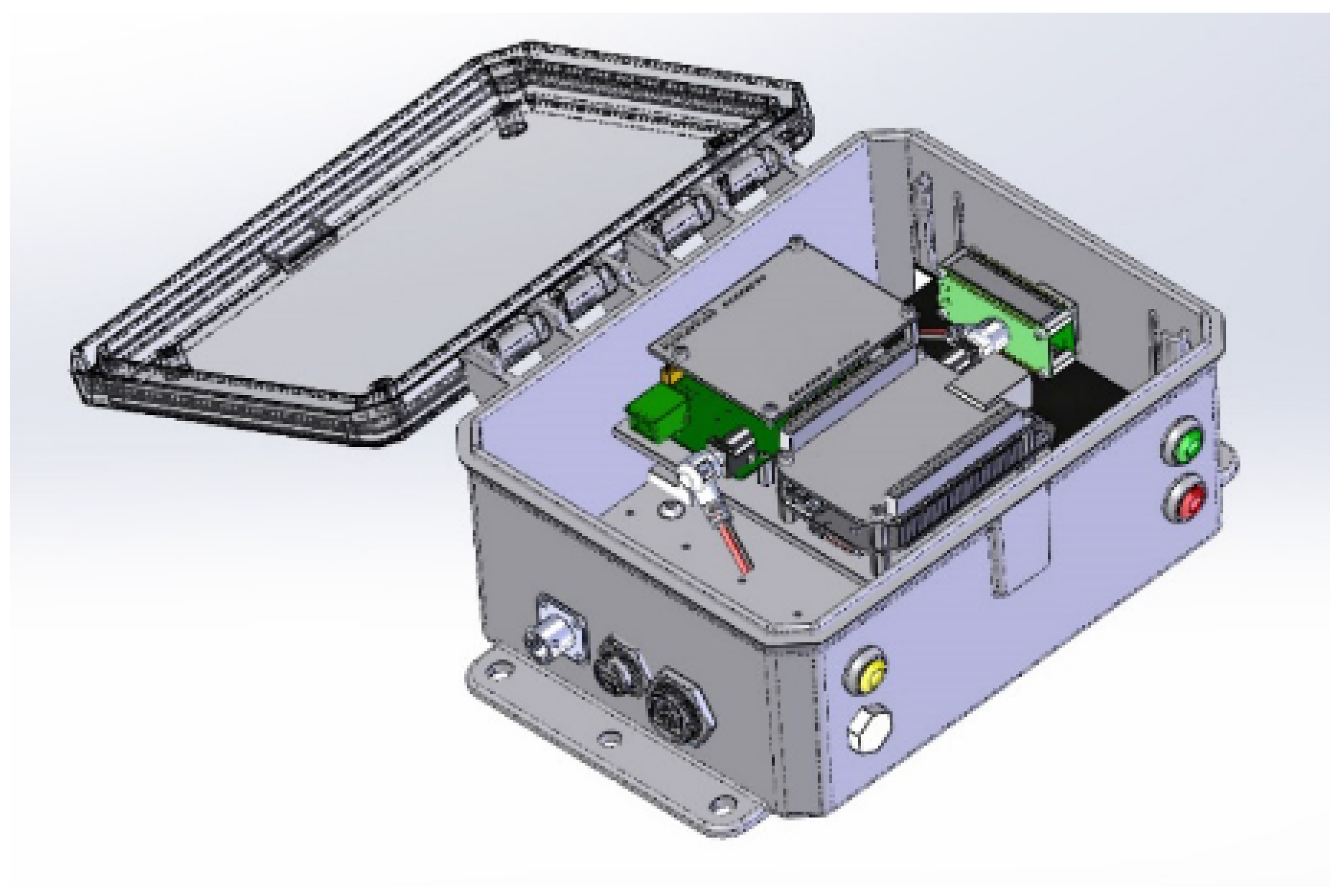
3.2. Merlyn Multisensor Platform

The Merlyn multisensor platform was used to collect nonradiological multisource data at a rate of 16 Hz. The Merlyn was designed by Special Technologies Laboratory, an organization within the Nevada National Security Site complex of facilities. A mockup of the Merlyn is shown in Figure 2.
The platform was built with a BeagleBone Black mainboard [17], an ATmega328P-based Arduino UNO breakout board [18], a ROHM SensorShield EVK-003 sensor package [19], and supporting hardware related to power distribution and data storage. The sensors housed on each Merlyn used in this work are listed in Table 2.

3.3. Data Products

To create the input data used for modeling, a series of preprocessing transformations were applied to the raw data streams collected by the Merlyn multisensors. First, each data stream was linearly interpolated such that measurements from different multisensors were assigned aligned timestamps. Since the data were recorded at 16 Hz and reactor operational state changes at a relatively slow rate, linear interpolation provides a reasonable approximation of the true measurement of the physical signal of interest for a given timestamp. After interpolation, the temperature and pressure data were background-subtracted using weather data collected from a nearby National Oceanic and Atmospheric Administration (NOAA) facility [25]. This mitigated potential confounding trends in the pressure and temperature features related to weather phenomena. Then, significant outliers were removed from each data stream by excluding spurious non-physical data larger than four mean average deviations to eliminate obvious measurement errors. After this, the x, y, and z components of the magnetometer and accelerometer for each multisensor were combined into a single data stream by taking the L2 norm of the individual coordinate components to obtain the vector magnitudes. Then, the mean and variance over 10 min time segments were taken for each data stream. This was a feature engineering step that increased the set of features to include both the average of and variability in the measured data for each sensing modality. Finally, the means and variances were standardized by taking the z-score of each data point so that features with different units of measurement were aligned to a common scale. This resulted in 120 features consisting of 60 means and 60 variances from 12 Merlyn multisensors over five sensing modalities and 39,745 total samples over the 40-week time series.
The multisensors experienced occasional periods of outage due to maintenance, power failures, and faulty components. These outages were treated as data that were missing completely at random [26] for preprocessing purposes. Missing data were substituted with the mean over the entire data stream time series, and an additional feature in the form of a “missing” flag for each data point set as 1 if the data were missing and 0 otherwise. This brought the total to 132 features consisting of 60 means, 60 variances, and 12 flags.
Information about nuclear reactor operational state was provided by the reactor operators in the form of core power output measured by diagnostic sensors in the primary coolant loop, which record data over the course of normal operations. A strict inequality at 0 MW to identify “reactor on” events would mislabel a substantial fraction of the data due to the measurement error of the diagnostic sensor. Instead, a boundary at 10% of maximum steady-state power (8.5 MW) was applied as this is the first of several partial-power holds during the normal HFIR startup procedure. Any potential discrepancies introduced in the labeling procedure based upon this assumption impact < 0.1 % of samples. These categorical ground truth data were used to interpolate reactor power state for each 10 min time segment corresponding to the samples on a fill-forward basis. Since the reactor transition states rarely occur over the 40-week time series, as can be seen in Figure 3, fill-forward interpolation adequately models the true reactor operational state for a given 10 min time segment.

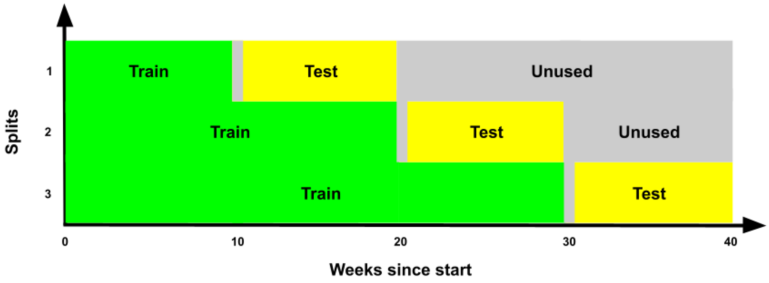
3.4. Data Partitioning

Given the temporal autocorrelation of the data, an assumption of independence between samples is incorrect, and therefore, the data set cannot be partitioned into training and testing sets using stratified sampling. Instead, the method of nested cross-validation was used [27]. In nested cross-validation, the time series is first partitioned into n time segments. These segments are organized into n 1 train/test splits by assigning the ith split the 0 , , i segments as training data and the i + 1 th segment as the test data set, where i = 1 , , n 1 . The training and testing scores for a given model are then taken as an average over the n 1 splits. A variant of nested cross-validation used in this work also inserts a buffer between the training and testing partitions to eliminate potential bias introduced by temporal autocorrelation across the training and testing partitions [28]. While this choice of data partitioning is nonrandom and can therefore introduce bias in estimating the true training and testing scores, this bias is likely smaller than the bias introduced by the presence of temporally autocorrelated samples in both the training and testing sets. Additionally, averaging performance metrics over each split produce estimates that mitigate nonrandom bias [27], although the extent of this mitigation is unknown.
The 40-week time series was split into four approximately equal-sized segments of 10,000 contiguous samples (the 4th segment contains 9745 samples), which correspond to approximately 10 weeks each. This size was chosen such that the train and test partition in each split contained one or more transitions between nuclear reactor power state while keeping the segments similarly sized. The proportion of “reactor on“ data points in each train and test set, respectively, is 0.55 and 0.48, 0.54 and 0.4, and 0.48 and 0.46. Hyperparameter optimization, which would reduce the number of test partitions from three to two for nested cross-validation and therefore increase bias in the estimates of the test scores, was not performed. A buffer of one week was placed between each training and testing partition to mitigate bias introduced by temporal autocorrelation. The approximate partitions for each of the three train/test splits are shown in the illustration in Figure 4. The scores reported in the following sections are averaged over the three splits.

3.5. Baseline Modeling Efforts

An HMM and a feed-forward neural network were trained and evaluated on the full feature set to generate the baseline performance of each model. TensorFlow [29], Scikit-learn [30], and HMMLearn [31] were used in conjunction with custom algorithms to perform the analyses in this work.
HMMs are stochastic state-space models [32]. They follow the first-order Markovian assumption that the state of a system at time t + 1 depends only on the state at time t and is independent of all preceding states. HMMs are fully defined by three parameters: initial hidden state probabilities, hidden-state transition probabilities, and class-conditional probability distributions.
For this problem, the HMM used two hidden states to represent the reactor’s operational status. It was assumed that the observations followed a multivariate Gaussian distribution to model the emissions from each hidden state. The HMM was trained by calculating the three parameters directly from the training data using maximum-likelihood estimation. Similar to calculating priors in Gaussian Discriminant Analysis, the initial hidden state probabilities were calculated by counting the frequency of each hidden state. Similarly, the hidden state transition probabilities were calculated by counting the frequency of each hidden state transition between timesteps. The class-conditional probability distributions were calculated by estimating a multivariate Gaussian distribution for each hidden state. Predictions with this HMM for testing were obtained using the Viterbi algorithm [33]. Given a sequence of observations from the testing set, the Viterbi algorithm uses dynamic programming to calculate the sequence of hidden states with the highest likelihood. The HMM trained on all the features achieved an accuracy of 0.583 . A plot of the predicted classes versus the actual classes over the three test partitions are shown for the HMM in Figure 5.
Feed-forward neural networks are deep-learning models used widely in machine learning [34]. They consist of an input layer, a user-specified number of hidden layers with user-specified widths, and an output layer. The number of neurons at the input layer of a neural network classifier is the same as the number of input features, whereas the output layer contains as many neurons as the number of classes, each corresponding to one of the possible classes. In this work, each layer is fully connected to the next. When input data are presented to the neural network, they are propagated through each layer, where they are weighted, summed, biased, and passed along to the next layer through a non-linear activation function. Using non-linear activation functions and hidden layers, neural networks can approximate arbitrary functions [35].
The feed-forward neural network used in this work had an architecture of six hidden layers with 250, 150, 90, 50, 30, and 20 neurons each with ReLU activation [36] (except for the last layer, which used softmax activation), used the Adam optimizer with an initial learning rate of 0.0001 [37], used cross-entropy loss with added L1 regularization set with the hyperparameter 0.001 to encourage sparsity [38], and ran for 100 epochs. The feed-forward neural network was trained by initializing the weights and biases to random values and then determining the optimal weights and biases at each layer using backpropagation [39]. While the traditional gradient-descent training technique was suitable for this demonstration, non-iterative training approaches may be employed in deployment scenarios to increase training speed while maintaining good generalizability [40,41]. Predictions were made using this feed-forward neural network by propagating the test set observations through each layer until it reached the output layer, where the class corresponding to the neuron with the highest softmax value was chosen as the predicted class.
The feed-forward neural network trained on all the features achieved an accuracy of 0.811 ± 0.005 averaged over 50 runs with different randomized initial weights. The statistical uncertainty was determined using standard error to construct a 95% confidence interval. A plot of the predicted classes versus the actual classes over the three test partitions is shown for a random trial run of the feed-forward neural network in Figure 6.

4. Feature Importance and Wrapper Methods

This work next provides a review of the application of feature importance methods to sensor data and introduces node and region importance methods as a model-agnostic means to achieve post hoc explainability for multisensor arrays.

4.1. Feature Importance

Node and region importance are closely related to feature importance, which measures how much individual features contribute to the overall performance of a model. Feature importance can provide insight into model explainability and aid in feature selection by distinguishing between features which do and do not contribute to increased model performance [42,43]. Feature importance has been used in many studies applying machine learning techniques to data collected by sensors to gain insight into explainability and feature selection. For example, permutation feature importance was used to measure sensor importance in a study classifying sitting posture to select a high-performing subset of features for a random forest model [44]. Gini importance and backward selection on a k-nearest neighbors model were used to eliminate irrelevant sensors in a study classifying the quality of a laser weld using features derived from sensor data [45]. Permutation feature importance was used to find the optimal placement of sensors on a circulation control wing for aircraft aerodynamics [46]. In addition, mutual information-based feature selection and genetic algorithm linear discriminant analysis feature selection were used to determine the most important features derived from sensor data for model-assisted fault detection [47]. More recently, novel feature importance methods based on weight changes were used to determine the relative importance of traffic features in deep belief networks regressing vehicle-collision frequency on a highway in Canada [48].

4.2. Wrapper Methods

While there are many feature importance methods designed for specific models such as out-of-bag permutation feature importance for random forests [49], SVM-RFE for support vector machines [50], integrated gradients for neural networks [51], and Vi-II/Vi-HI for deep belief networks [48], this work focuses on a class of feature importance methods called wrapper methods, which “wrap” around the model to measure the importance of individual features [52]. The key benefit of wrapper methods is that they can be applied to any model in any context to measure feature importance. The specific wrapper methods considered here are Leave One Covariate Out (LOCO) [53] and Forward Feature Selection (FFS) [42]. In LOCO, the feature importance of the ith feature is measured as the difference in accuracy between a model trained on a full set of features and a model trained on all the features except for the ith feature. In FFS, candidate features are iteratively added to a working set of features by greedily adding the candidate feature, achieving the highest accuracy for the working set at each iteration. The order in which features are added to the working set provides a ranking of feature importance.

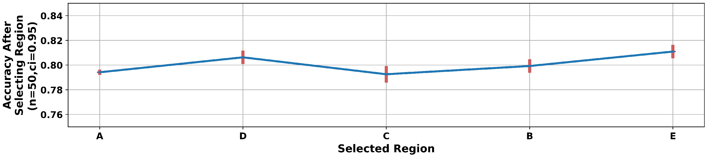
4.3. Node and Region Importance

Node and region importance extend traditional concepts of feature importance by directly measuring how much a group of features derived from a node or region, considered in tandem, contribute to the overall performance of a model. That is, LOCO and FFS may be defined as wrapper methods for node and region importance by grouping features derived from single nodes and spatially collocated sets of nodes. More specifically, LOCO is extended to Leave One Node Out (LONO) by measuring the importance of the ith node as the difference in accuracy between a model trained on the full set of features derived from the full set of nodes and a model trained on the full set of features except for features derived from the ith node. Leave One Region Out (LORO), Forward Node Selection (FNS), and Forward Region Selection (FRS) are similarly defined. Although initial efforts in measuring the importance of a group of features have been made for models such as random forests [54], multilayer perceptrons [55], support vector machines [56], and least squares regression [57], the spatial importance algorithms introduced in this work provide a means for measuring node and region importance that can be applied to any model.
While it is possible to measure node and region importance by measuring the importances of the individual constituent features and adding them together, it has been shown that the importance of a group of features is given by the sum of the importances of the individual features only if the features are uncorrelated, which is unrealistic for many practical settings [54]. Feature covariance is especially relevant for data collected by multisensor networks where there are many potential sources of correlation. For example, there is correlation between different but related sensing modalities on a single node and between the same sensing modality across two different, nearby nodes. Given this fact, node and region importance provide strong advantages over measuring the importances of individual features and considering the individual importances in a group when evaluating the impact of a given node or region on a classification problem. A limitation remains in that node and region correlations are likely to result in nodes and regions contributing different amounts of information to the classification problem when considered jointly versus in isolation [58]. While covariates may be identified through pairwise, iterative analyses, there is a combinatorial explosion in the required number of trials, rendering such approaches intractable in the general case.

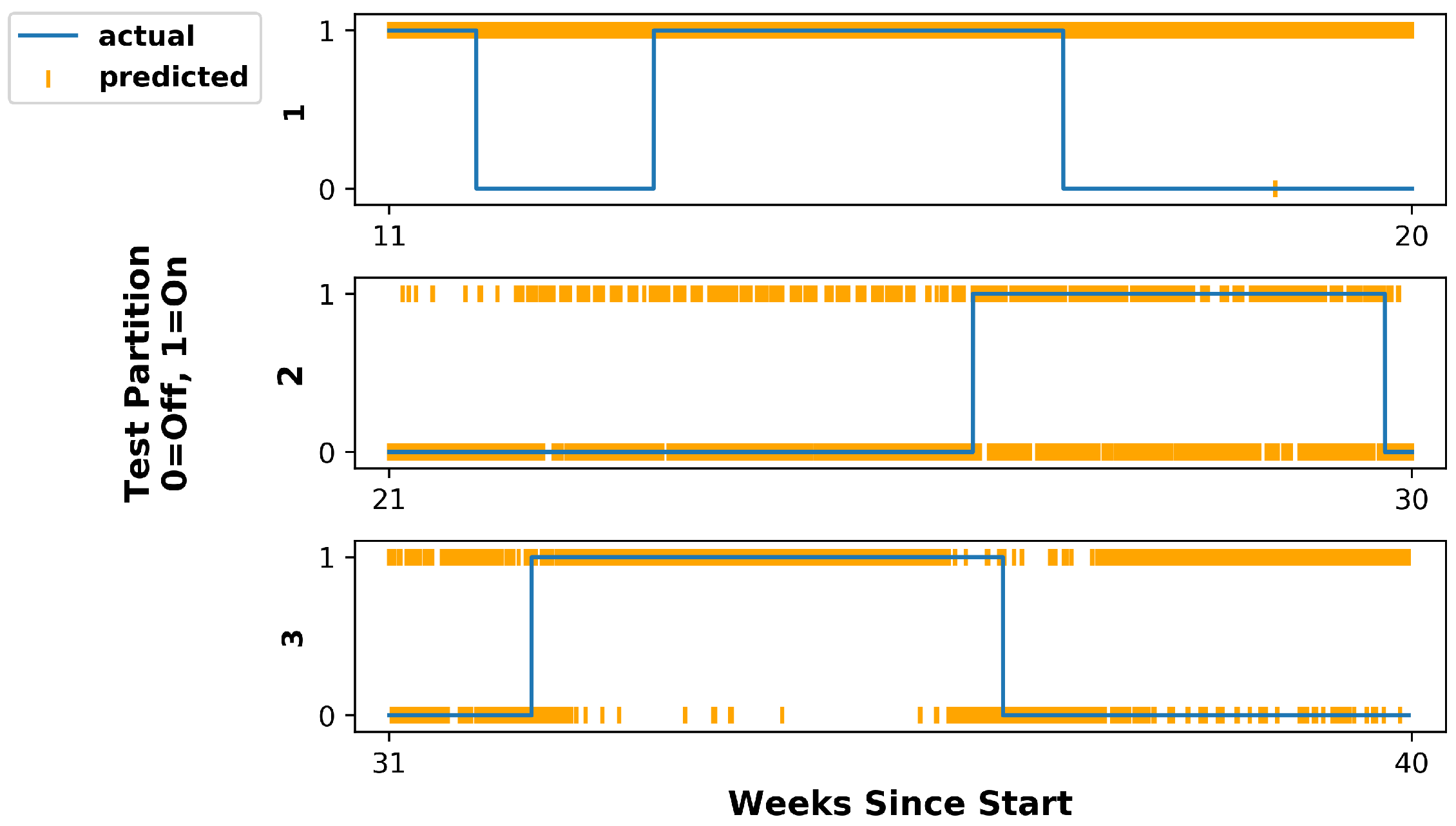
5. Analysis and Results

Next, the performance of the spatial importance algorithms is evaluated by addressing the question of which nodes and regions of the multisensor network are the most important for enabling the accurate prediction of nuclear reactor operational state.

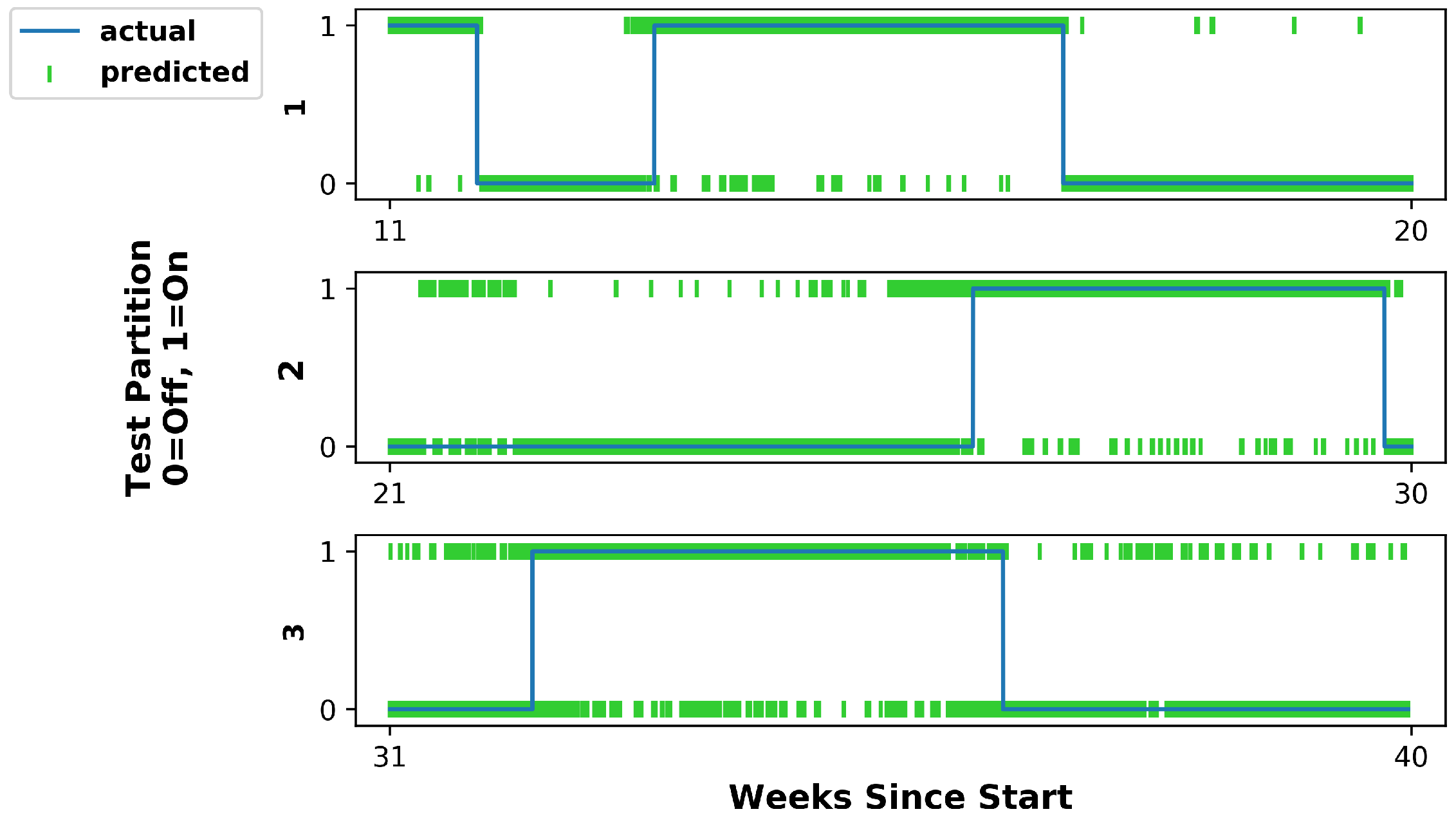
5.1. Hidden Markov Model

Figure 7 is a plot of the accuracy differences obtained through LONO analysis applied to the HMM. The differences in accuracy between the model trained on the full set of features and the model trained on all the features except for those derived from the ith node are ordered from top to bottom in order of highest positive accuracy difference (i.e., most important) to largest negative accuracy difference (i.e., most confounding). From this plot, it can be seen that Node 9 had a strong positive impact on model accuracy. On the other hand, Node 2 had a strong negative impact on model accuracy.
Figure 8 is a plot of the accuracy differences obtained through LORO analysis applied to the HMM. From this plot, Region A was identified as having a strong positive impact on model accuracy, whereas Regions E and C were identified as having negative impacts on model accuracy.
Figure 9 is a plot of the accuracy obtained after adding each node to the working set of nodes during FNS analysis applied to the HMM. The nodes are ordered by importance as determined based on node selection into the working set during the execution of the algorithm (i.e., the node that provides the highest accuracy is selected at each iteration). From this plot, it can be seen that Node 6 was the most important node. Conversely, Nodes 5, 4, and 2 were ranked of lowest importance in this analysis. Additionally, model accuracy decreased when Nodes 5, 4, and 2 were selected, which indicates that these nodes have a negative impact on model accuracy. Interestingly, the two most important nodes (Nodes 6 and 9) and four least important nodes (Nodes 2, 4, 5, and 7) are similarly identified in the FNS and LONO analyses.
Figure 10 is a plot of the accuracy obtained after each region was added to the working set of regions during FRS analysis applied to the HMM. From this plot, Region A was ranked most important, whereas Regions C and E were ranked of least importance. In the case of the latter, their selection resulted in decreased model accuracy, indicating that these regions have a negative impact on model accuracy.
These analyses offer valuable insight relevant to feature selection. After evaluating all the models from these four analyses, it can be seen from the FNS analysis that model performance can be increased significantly by only training on features derived from Nodes 6, 9, and 1. An HMM trained only on this subset of nodes resulted in a test accuracy of 0.839 , which is a significant improvement over the baseline accuracy of 0.583 . Plots of the predicted classes versus the actual classes over the three test data partitions for the improved HMM are shown in Figure 11.

5.2. Feed-Forward Neural Network

Figure 12 is a plot of the accuracy differences obtained through LONO analysis applied to the feed-forward neural network. For both the baseline full feature set and the feature set with all the features except for those derived from the ith node, the process of training and evaluating a model was repeated for 50 trials to determine the statistical uncertainty in the assessment. A 95% confidence interval was determined using standard error for the accuracy differences for each excluded node. From this plot, Nodes 6 and 9 were identified as having positive impacts on model accuracy, whereas Node 7 had a strong negative impact on model accuracy. Similarly, Figure 13 is a plot of the accuracy differences obtained through LORO analysis applied to the feed-forward neural network. From this plot, it can be seen that Region A had a strong positive impact on model accuracy.
Figure 14 is a plot of the accuracy obtained after adding each node to the working set of nodes during FNS analysis applied to the feed-forward neural network. The performance of a candidate node was taken as the average over 50 trials with randomized initial weights. The 95% confidence interval for each selected candidate node is shown in the plot. From this analysis, Node 6 was ranked most important. Node 7 was ranked of least importance as it was selected last. Additionally, the selection of Node 7 resulted in a significant accuracy decrease after its addition into the working set, indicating that it has a negative impact on model accuracy.
Figure 15 is a plot of the accuracy obtained after adding each region to the working set of regions during FRS analysis applied to the feed-forward neural network. From this analysis, Region A was ranked as most important. Additionally, an analysis of the candidate scores from the first iteration of the FRS analysis shown in Table 3 demonstrates that Region A had a significantly higher impact on model accuracy in comparison to other regions.
Similar to the improved HMM, the FNS analysis demonstrates that model performance can be increased by only training on features derived from Nodes 6, 10, 1, 8, 4, 5, and 12. A feed-forward neural network trained 50 times with different randomized initial weights on this subset of nodes resulted in an average test accuracy of 0.884 ± 0.004 , where the error bars represent a 95% confidence interval. This provides a statistically significant improvement over the baseline average test accuracy of 0.811 ± 0.005 . Plots of the predicted classes versus the actual classes over the three test partitions for the improved feed-forward neural network are shown in Figure 16.

5.3. Discussion

These analyses offer valuable insight regarding operations at the HFIR facility as well as to the performance of the spatial importance algorithms. For example, Nodes 6 and 9 as well as Region A were identified as having strong positive impacts on model accuracy for both the HMM and feed-forward neural network. The corresponding area contains the reactor cooling tower, pointing to a potential causal relationship between the cooling tower and reactor operational state. This result is consistent with basic nuclear engineering principles: power generation on a megawatt-or-greater scale, which includes nearly all research reactors (1 to a few MW), HFIR (85 MW), and reactors used for commercial power generation (1–3 GW), necessitates operation of a significant cooling system for the conveyance and removal of heat from the reactor core [59]. This is traditionally accomplished using a primary coolant loop to remove heat from the fuel elements and a secondary loop that receives heat—but not coolant—via a heat exchanger to provide defense-in-depth containment against radioisotope emissions. While the pumps driving the primary system are collocated with the core, the secondary pumps are often located away from the containment building, instead residing near the heat-rejection apparatus (e.g., the iconic hyperbolic cooling towers), where they are easier to access for maintenance. These secondary pumps produce signals intrinsically related to, but distinct from, the reactor core, such as local magnetic fields that may be recorded by the magnetometer and vibrations that may be detected by the accelerometer. The heat rejection into the environment also produces local temperature perturbations that may be sensed by the thermometer. In short, node and region importance analyses, combined with knowledge of the HFIR facility and nuclear reactor operations, provide justification for a causal relationship between cooling tower operations and the nuclear reactor’s operational state.
Further exploration of this hypothesis was carried out using a decision tree [60], an inherently explainable and relatively simple machine learning model in comparison to a neural network. Using features derived solely from Node 9, the Gini importance of each feature was evaluated to obtain an importance metric that quantifies the overall information gain from a feature throughout the tree, with higher scores implying greater importance of the feature to the model predictions. The decision tree achieved a mean accuracy of 0.743 over the test partitions (significantly less than the average accuracy of the neural network, 0.884 ± 0.004 , achieved by training on features collected at seven nodes). The average Gini importances for each feature over the test partitions are shown in Table 4. The magnetic field variance was observed to be significantly more important than the other features, followed by acceleration mean and pressure mean, respectively. These importance scores further support the conjecture regarding the physical indicators associated with the secondary pumps and fans at the HFIR cooling tower.
Additionally, Nodes 2, 4, and 5, Region C (an area with office buildings), and Region E (the main entrance to the facility) were identified as having negative impacts on model accuracy in the analyses applied to the HMM. These are areas of high foot and vehicle traffic, suggesting that foot and vehicle traffic may produce noise in the data, which reduces the accuracy of the HMM. Foot and vehicle traffic produce vibrations that may be recorded by the accelerometer and—for vehicles—transient distortions to the local magnetic field that may be detected by the magnetometer. There is no clear relationship between foot and vehicle traffic in these areas and nuclear reactor operational state at HFIR. This suggests that foot and vehicle traffic may negatively affect the performance of the HMM predicting the nuclear reactor’s operational state. This likely did not affect the feed-forward neural network model performance due to the L1 regularization applied to the loss function, which encouraged sparsity in the model parameters and suppressed noise.
In addition to gains arising from feature selection, another potential explanation for the improved HMM performance when using select nodes is suggested by the differences in predictions on the test partitions between the baseline and improved HMM. That is, the baseline model transitioned between states (except when it only predicted one class) much more often than the improved model transitioned between states. It is possible that the class-conditional probabilities overwhelmed the values contributed by the transition matrix when calculating the predicted state in the baseline HMM. This outcome is consistent with results found in Bayes classifiers trained on high-dimensional data [61]. Given that this issue is mitigated as the dimensionality of the data decreases, the removal of nodes may have significantly reduced the rate of transitions and increased overall accuracy in the improved HMM.
Node 7 was identified, using both LONO and FNS analysis, as having a strong negative impact on model accuracy in the feed-forward neural network. A long outage period occurred at Node 7 during the data collection campaign (Weeks 22 40 ) due to a component failure, which likely impacted its importance ranking. In the same way in which it has been shown that perturbations in test data sets can dramatically change predictions in adversarial scenarios for neural networks [62], the sensor outage on Node 7 during the evaluation of the second and third test sets, which affected a significant number of features, could have dramatically changed the performance of the model. This issue might be mitigated by a more sophisticated method of filling in the missing data, such as nearest neighbor [63] or kriging [64] approaches.
As with most other forward- or backward-selection interpretation methods, feature correlation represents a potential source of bias that may impact assessments of node and region importance [58]. As such, spatial importance assessments were made based upon the application of multiple complementary methods in conjunction with the known physical causal relationships between cooling tower operations and reactor power level. While a robust node and region ranking assessment would require a thorough multivariate correlation analysis [65], it is notable that the most important nodes and regions identified in this work are consistent across models and methods. That is, for both the HMM and feed-forward neural network and using both the leave-one-out and forward-selection approaches, Nodes 6 and 9 and Region A were consistently identified as important.

6. Summary and Conclusions

Using data collected by a multisensor network, node and region importance methods were demonstrated on a problem predicting a nuclear reactor’s operational state with a hidden Markov model and a feed-forward neural network. First, base models were created, and then these models were analyzed using node and region importance, and finally the models were improved with feature selection.
The accuracy of the HMM was increased from 0.583 to 0.839 through feature selection informed by node and region importance. Node and region importance analyses also demonstrated that the HMM was potentially sensitive to noise in the data produced by high foot and vehicle traffic and/or the high dimensionality of the data, which reduced model performance. Similarly the accuracy of the feed-forward neural network was increased from 0.811 ± 0.005 to 0.884 ± 0.004 through feature selection, where the error bars are representative of a 95% confidence interval produced by training and evaluating a feed-forward neural network for 50 trials with different randomized initial weights and averaging the results. The results from node and region importance analyses suggested the feed-forward neural network was sensitive to a sensor outage caused by a sensor component failure that reduced model performance when missing data were filled in with a mean over the time series and an additional “missing” flag. Additionally, node and region importance provided evidence of a potential causal relationship between reactor operational state and cooling tower operations at the facility, increasing understanding of the problem context and the predictive models.
The node and region importance methods outlined herein can be applied in any context where sensors are deployed over a spatial area to record data streams used to build predictive machine learning models. Since they are extensions of wrapper methods, they can be applied to any machine learning model, whether it be for classification or regression, without loss of generality. These methods can be used to identify nodes and regions with strong positive and negative impacts on accuracy, which can in turn be used to enhance insight into the problem context, better understand the models generated from sensor network data, and improve model performance through feature selection. While the ability to achieve a robust feature ranking is limited by variable correlation across nodes and regions, consistency across different models and methods can provide strong evidence to support inferential hypotheses regarding the physical systems. Node and region importance helps nontechnical users such as policymakers and analysts better trust the predictions and understand the limitations of an otherwise opaque model applied to sensor network data by providing insight into which nodes and regions drive model performance.

Author Contributions

Conceptualization, J.T. and B.L.G.; methodology, J.T. and B.L.G.; software, J.T. and C.S.; validation, J.T., C.S. and A.H.; formal analysis, J.T.; investigation, J.T., C.S. and A.H.; resources, C.S. and B.L.G.; data curation, C.S.; writing—original draft preparation, J.T. and B.L.G.; writing—review and editing, J.T., B.L.G., C.S. and A.H.; visualization, J.T.; supervision, B.L.G.; project administration, B.L.G.; funding acquisition, B.L.G. All authors have read and agreed to the published version of the manuscript.

Funding

This work was performed under the auspices of the U.S. Department of Energy by Lawrence Berkeley National Laboratory under Contract DE-AC02-05CH11231 and by the University of California, Berkeley, through the Nuclear Science and Security Consortium under Award DE-NA0003180. The project was funded by the U.S. Department of Energy, National Nuclear Security Administration, Office of Defense Nuclear Nonproliferation Research and Development (DNN R&D).

Institutional Review Board Statement

Not applicable.

Informed Consent Statement

Not applicable.

Data Availability Statement

Restrictions apply to the availability of these data. Data were generated at Oak Ridge National Laboratory and are available from the authors with the permission of the U.S. Department of Energy, National Nuclear Security Administration, Office of Defense Nuclear Nonproliferation Research and Development.

Acknowledgments

The authors thank the MINOS Venture and the Oak Ridge National Laboratory Staff at the High Flux Isotope Reactor, especially Jared Johnson, Will Ray, Randall Wetherington, and Michael Willis, for their help in performing these experiments. Thanks also to Stuart Russell for expert advice and the Complexity Group at the University of California, Berkeley, for useful discussions.

Conflicts of Interest

The authors declare no conflict of interest.

Abbreviations

The following abbreviations are used in this manuscript:
FFSForward Feature Selection
FNSForward Node Selection
FRSForward Region Selection
HMMHidden Markov Model
HFIRHigh Flux Isotope Reactor
LOCOLeave One Covariate Out
LONOLeave One Node Out
LOROLeave One Region Out
NOAANational Oceanic and Atmospheric Administration

References

  1. Abe, N. The NPT at Fifty: Successes and Failures. J. Peace Nucl. Disarm. 2020, 3, 224–233. [Google Scholar] [CrossRef]
  2. Gastelum, Z.; Goldblum, B.; Shead, T.; Stewart, C.; Miller, K.; Luttman, A. Integrating Physical and Informational Sensing to Support Nonproliferation Assessments of Nuclear-Related Facilities. In Proceedings of the Institute of Nuclear Materials Management (INMM) 60th Annual Meeting, Palm Springs, CA, USA, 14–18 July 2019; pp. 1–10. [Google Scholar]
  3. Stewart, C.L.; Goldblum, B.L.; Tsai, Y.A.; Chockkalingam, S.; Padhy, S.; Wright, A. Multimodal Data Analytics for Nuclear Facility Monitoring. In Proceedings of the Institute of Nuclear Materials Management (INMM) 60th Annual Meeting, Palm Springs, CA, USA, 14–18 July 2019; pp. 1–10. [Google Scholar]
  4. Ramirez, C.; Rao, N.S.V. Reactor Facility Operational State Classification Using Gas Effluents and Radiation Measurements. In Proceedings of the 2018 IEEE Nuclear Science Symposium and Medical Imaging Conference Proceedings (NSS/MIC), Sydney, NSW, Australia, 10–17 November 2018; pp. 1–2. [Google Scholar] [CrossRef]
  5. Ramirez, C.; Rao, N.S.V. Facility On/Off Inference by Fusing Multiple Effluence Measurements. In Proceedings of the 2017 IEEE Nuclear Science Symposium and Medical Imaging Conference (NSS/MIC), Atlanta, GA, USA, 21–28 October 2017; pp. 1–4. [Google Scholar] [CrossRef]
  6. Flynn, G.; Parikh, N.K.; Egid, A.; Casleton, E. Predicting the Power Level of a Nuclear Reactor by Combining Multiple Modalities. In Proceedings of the Institute of Nuclear Materials Management (INMM) 60th Annual Meeting, Palm Springs, CA, USA, 14–18 July 2019; pp. 1–10. [Google Scholar]
  7. Parikh, N.; Flynn, G.; Casleton, E.; Archer, D.; Karnowski, T.; Nicholson, A.; Maceira, M.; Marcillo, O.; Ray, W.; Wetherington, R. Predicting the Power Level of a Nuclear Reactor using a Time Series-based Approach. In Proceedings of the Institute of Nuclear Materials Management (INMM) 61st Annual Meeting, Online, 12–16 July 2020. [Google Scholar]
  8. Parikh, N.; Flynn, G.; Archer, D.; Karnowski, T.; Maceira, M.; Marcillo, O.; Ray, W.; Wetherington, R.; Willis, M.; Nicholson, A. Data and Model Selection to Detect Sparse Events from Multiple Sensor Modalities. In Proceedings of the 2021 INMM and ESARDA Joint Annual Meeting, Online, 23–26, 30 August–1 September 2021. [Google Scholar]
  9. Rao, N.S.V.; Greulich, C.; Sen, S.; Dayman, K.J.; Hite, J.; Ray, W.; Hale, R.; Nicholson, A.D.; Johnson, J.; Hunley, R.D.; et al. Reactor Power Level Estimation by Fusing Multi-Modal Sensor Measurements. In Proceedings of the 2020 IEEE 23rd International Conference on Information Fusion (FUSION), Rustenburg, South Africa, 6–9 July 2020; pp. 1–8. [Google Scholar] [CrossRef]
  10. Chai, C.; Ramirez, C.; Maceira, M.; Marcillo, O. Monitoring Operational States of a Nuclear Reactor Using Seismoacoustic Signatures and Machine Learning. Seismol. Res. Lett. 2022, 93, 1660–1672. [Google Scholar] [CrossRef]
  11. Schmidt, E.; Work, R.; Catz, S.; Horvitz, E.; Chien, S.; Jassy, A.; Clyburn, M.; Louie, G.; Darby, C.; Mark, W.; et al. Final Report; National Security Commission on Artificial Intelligence: Washington, DC, USA, 2021. [Google Scholar]
  12. Adadi, A.; Berrada, M. Peeking Inside the Black-Box: A Survey on Explainable Artificial Intelligence (XAI). IEEE Access 2018, 6, 52138–52160. [Google Scholar] [CrossRef]
  13. Lipton, Z.C. The Mythos of Model Interpretability: In Machine Learning, the Concept of Interpretability is Both Important and Slippery. Queue 2018, 16, 31–57. [Google Scholar] [CrossRef]
  14. Barredo Arrieta, A.; Díaz-Rodríguez, N.; Del Ser, J.; Bennetot, A.; Tabik, S.; Barbado, A.; Garcia, S.; Gil-Lopez, S.; Molina, D.; Benjamins, R.; et al. Explainable Artificial Intelligence (XAI): Concepts, taxonomies, opportunities and challenges toward responsible AI. Inf. Fusion 2020, 58, 82–115. [Google Scholar] [CrossRef]
  15. Chandler, D.; Betzler, B.R.; Davidson, E.; Ilas, G. Modeling and simulation of a High Flux Isotope Reactor representative core model for updated performance and safety basis assessments. Nucl. Eng. Des. 2020, 366, 110752. [Google Scholar] [CrossRef]
  16. Robinson, S.M.; Benker, D.E.; Collins, E.D.; Ezold, J.G.; Garrison, J.R.; Hogle, S.L. Production of Cf-252 and other transplutonium isotopes at Oak Ridge National Laboratory. Radiochim. Acta 2020, 108, 737–746. [Google Scholar] [CrossRef]
  17. Coley, G. BeagleBone Black System Reference Manual. Beagleboard. Rev. C.1. 2014. Available online: https://cdn.sparkfun.com/datasheets/Dev/Beagle/BBB_SRM_C.pdf (accessed on 15 April 2019).
  18. Atmel Corporation. 8-bit AVR Microcontroller with 32K Bytes In-System Programmable Flash. Rev. 7810D-AVR-01/15. 2015. Available online: https://ww1.microchip.com/downloads/en/DeviceDoc/Atmel-7810-Automotive-Microcontrollers-ATmega328P_Datasheet.pdf (accessed on 15 April 2019).
  19. ROHM Semiconductor. SensorShield-EVK-003 Manual. Rev.001. 2018. Available online: http://rohmfs.rohm.com/en/products/databook/applinote/ic/sensor/sensorshield-evk-003_ug-e.pdf (accessed on 15 April 2019).
  20. Kionix. 8g/16g/32g Tri-axis Digital Accelerometer Specifications. Rev. 2.0. 2017. Available online: https://d10bqar0tuhard.cloudfront.net/en/datasheet/KX224-1053-Specifications-Rev-2.0.pdf (accessed on 15 April 2019).
  21. ROHM Semiconductor. Optical Proximity Sensor and Ambient Light Sensor with IrLED. Rev.001. 2016. Available online: https://fscdn.rohm.com/en/products/databook/datasheet/opto/optical_sensor/opto_module/rpr-0521rs-e.pdf (accessed on 15 April 2019).
  22. ROHM Semiconductor. Magnetic Sensor Series: 3-Axis Digital Magnetometer IC. Rev.001. 2016. Available online: https://fscdn.rohm.com/en/products/databook/datasheet/ic/sensor/geomagnetic/bm1422agmv-e.pdf (accessed on 15 April 2019).
  23. ROHM Semiconductor. Pressure Sensor Series: Pressure Sensor IC. Rev.003. 2016. Available online: https://fscdn.rohm.com/en/products/databook/datasheet/ic/sensor/pressure/bm1383aglv-e.pdf (accessed on 15 April 2019).
  24. ROHM Semiconductor. Temperature Sensor IC. Rev.001. 2015. Available online: https://fscdn.rohm.com/en/products/databook/datasheet/ic/sensor/temperature/bd1020hfv-e.pdf (accessed on 15 April 2019).
  25. NOAA. Climate Data Online. 2021. Available online: https://www.ncdc.noaa.gov/cdo-web/ (accessed on 19 April 2020).
  26. Rubin, D. Inference and missing data. Biometrika 1976, 63, 581–592. [Google Scholar] [CrossRef]
  27. Varma, S.; Simon, R. Bias in error estimation when using cross-validation for model selection. BMC Bioinform. 2006, 7, 91. [Google Scholar] [CrossRef] [PubMed]
  28. Roberts, D.; Bahn, V.; Ciuti, S.; Boyce, M.; Elith, J.; Guillera-Arroita, G.; Hauenstein, S.; Lahoz-Monfort, J.; Schröder, B.; Thuiller, W.; et al. Cross-validation strategies for data with temporal, spatial, hierarchical, or phylogenetic structure. Ecography 2017, 40, 913–929. [Google Scholar] [CrossRef]
  29. Abadi, M.; Agarwal, A.; Barham, P.; Brevdo, E.; Chen, Z.; Citro, C.; Corrado, G.S.; Davis, A.; Dean, J.; Devin, M.; et al. TensorFlow: Large-Scale Machine Learning on Heterogeneous Systems. Software. 2015. Available online: tensorflow.org (accessed on 15 April 2019).
  30. Pedregosa, F.; Varoquaux, G.; Gramfort, A.; Michel, V.; Thirion, B.; Grisel, O.; Blondel, M.; Prettenhofer, P.; Weiss, R.; Dubourg, V.; et al. Scikit-learn: Machine Learning in Python. J. Mach. Learn. Res. 2011, 12, 2825–2830. [Google Scholar]
  31. HMMLearn. Available online: http://hmmlearn.readthedocs.org/ (accessed on 19 April 2021).
  32. Seymore, K.; McCallum, A.; Rosenfeld, R. Learning Hidden Markov Model Structure for Information Extraction. In Proceedings of the Association for the Advancement of Artificial Intelligence (AAAI) ’99 Workshop on Machine Learning for Information Extraction, Orlando, FL, USA, 18–19 July 1999; pp. 37–42. [Google Scholar]
  33. Forney, G. The Viterbi algorithm. Proc. IEEE 1973, 61, 268–278. [Google Scholar] [CrossRef]
  34. Sazli, M. A brief review of feed-forward neural networks. Commun. Fac. Sci. Univ. Ank. Ser. A2–A3 2006, 50, 11–17. [Google Scholar] [CrossRef]
  35. Hornik, K.; Stinchcombe, M.; White, H. Multilayer feedforward networks are universal approximators. Neural Netw. 1989, 2, 359–366. [Google Scholar] [CrossRef]
  36. Nair, V.; Hinton, G.E. Rectified Linear Units Improve Restricted Boltzmann Machines. In Proceedings of the 27th International Conference on Machine Learning (ICML’10), Haifa, Israel, 21–24 June 2010; Omnipress: Madison, WI, USA, 2010; pp. 807–814. [Google Scholar]
  37. Kingma, D.P.; Ba, J. Adam: A Method for Stochastic Optimization. In Proceedings of the 3rd International Conference on Learning Representations, ICLR 2015, San Diego, CA, USA, 7–9 May 2015; Bengio, Y., LeCun, Y., Eds.; Conference Track Proceedings: Ithaca, NY, USA, 2015; pp. 1–10. [Google Scholar]
  38. Bach, F.; Jenatton, R.; Mairal, J.; Obozinski, G. Convex Optimization with Sparsity-Inducing Norms. In Optimization for Machine Learning; The MIT Press: Cambridge, MA, USA, 2011; Volume 5, pp. 19–53. [Google Scholar]
  39. Hecht-Nielsen, R. Theory of the Backpropagation Neural Network. In Proceedings of the International Joint Conference on Neural Networks (IJCNN), Washington, DC, USA, 18–22 June 1989; IEEE: Piscataway, NJ, USA, 1989; Volume 1, pp. 593–605. [Google Scholar] [CrossRef]
  40. Wang, X.; Cao, W. Non-iterative approaches in training feed-forward neural networks and their applications. Soft Comput. 2018, 22, 3473–3476. [Google Scholar] [CrossRef]
  41. Cao, W.; Wang, X.; Ming, Z.; Gao, J. A review on neural networks with random weights. Neurocomputing 2018, 275, 278–287. [Google Scholar] [CrossRef]
  42. Guyon, I.; Elisseeff, A. An Introduction to Variable and Feature Selection. J. Mach. Learn. Res. 2003, 3, 1157–1182. [Google Scholar]
  43. Gevrey, M.; Dimopoulos, I.; Lek, S. Review and comparison of methods to study the contribution of variables in artificial neural network models. Ecol. Model. 2003, 160, 249–264. [Google Scholar] [CrossRef]
  44. Zemp, R.; Tanadini, M.; Plüss, S.; Schnüriger, K.; Singh, N.; Taylor, W.; Lorenzetti, S. Application of Machine Learning Approaches for Classifying Sitting Posture Based on Force and Acceleration Sensors. BioMed Res. Int. 2016, 2016, 5978489. [Google Scholar] [CrossRef]
  45. Knaak, C.; Thombansen, U.; Abels, P.; Kröger, M. Machine learning as a comparative tool to determine the relevance of signal features in laser welding. Procedia CIRP 2018, 74, 623–627. [Google Scholar] [CrossRef]
  46. Semaan, R. Optimal sensor placement using machine learning. Comput. Fluids 2017, 159, 167–176. [Google Scholar] [CrossRef]
  47. Han, H.; Gu, B.; Wang, T.; Li, Z. Important sensors for chiller fault detection and diagnosis (FDD) from the perspective of feature selection and machine learning. Int. J. Refrig. 2011, 34, 586–599. [Google Scholar] [CrossRef]
  48. Chen, Q.; Pan, G.; Chena, W.; Wu, P. A Novel Explainable Deep Belief Network Framework and Its Application for Feature Importance Analysis. IEEE Sens. J. 2021, 21, 25001–25009. [Google Scholar] [CrossRef]
  49. Breiman, L. Random Forests. Mach. Learn. 2001, 45, 5–32. [Google Scholar] [CrossRef]
  50. Guyon, I.; Weston, J.; Barnhill, S.; Vapnik, V. Gene Selection for Cancer Classification using Support Vector Machines. Mach. Learn. 2002, 46, 389–422. [Google Scholar] [CrossRef]
  51. Sundararajan, M.; Taly, A.; Yan, Q. Axiomatic Attribution for Deep Networks. In Proceedings of the 34th International Conference on Machine Learning, Sydney, Australia, 6–11 August 2017. [Google Scholar]
  52. Kohavi, R.; John, G. Wrappers for feature subset selection. Artif. Intell. 1997, 97, 273–324. [Google Scholar] [CrossRef]
  53. Lei, J.; G’Sell, M.; Rinaldo, A.; Tibshirani, R.; Wasserman, L. Distribution-Free Predictive Inference for Regression. J. Am. Stat. Assoc. 2018, 113, 1094–1111. [Google Scholar] [CrossRef]
  54. Gregorutti, B.; Michel, B.; Saint-Pierre, P. Grouped variable importance with random forests and application to multiple functional data analysis. Comput. Stat. Data Anal. 2015, 90, 15–35. [Google Scholar] [CrossRef] [Green Version]
  55. Chakraborty, D.; Pal, N. Selecting Useful Groups of Features in a Connectionist Framework. IEEE Trans. Neural Networks 2008, 19, 381–396. [Google Scholar] [CrossRef]
  56. Zhang, H.; Liu, Y.; Wu, Y.; Zhu, J. Variable selection for the multicategory SVM via adaptive sup-norm regularization. Electron. J. Stat. 2008, 2, 149–167. [Google Scholar] [CrossRef]
  57. Yuan, M.; Lin, Y. Model selection and estimation in regression with grouped variables. J. R. Stat. Soc. Ser. B Statist. Methodol. 2006, 68, 49–67. [Google Scholar] [CrossRef]
  58. Covert, I.; Lundberg, S.; Lee, S. Understanding Global Feature Contributions With Additive Importance Measures. In Advances in Neural Information Processing Systems; Larochelle, H., Ranzato, M., Hadsell, R., Balcan, M.F., Lin, H., Eds.; Curran Associates, Inc.: Red Hook, NY, USA, 2020; Volume 33, pp. 17212–17223. [Google Scholar]
  59. Hensley, J. Cooling Tower Fundamentals, 2nd ed.; SPX Cooling Technologies, Inc.: Overland Park, KS, USA, 2009. [Google Scholar]
  60. Breiman, L.; Friedman, J.; Olshen, R.; Stone, C. Classification Furthermore, Regression Trees, 1st ed.; Routledge: New York, NY, USA, 1984. [Google Scholar]
  61. Bennett, P. Assessing the Calibration of Naive Bayes Posterior Estimates; Technical Report CMU-CS-00-155; Computer Science Department, School of Computer Science, Carnegie Mellon University: Pittsburgh, PA, USA, 2000. [Google Scholar]
  62. Carlini, N.; Wagner, D. Towards Evaluating the Robustness of Neural Networks. In Proceedings of the 2017 IEEE Symposium on Security and Privacy (SP), San Jose, CA, USA, 22–26 May 2017; IEEE Computer Society: Los Alamitos, CA, USA, 2017; pp. 39–57. [Google Scholar] [CrossRef]
  63. Beretta, L.; Santaniello, A. Nearest neighbor imputation algorithms: A critical evaluation. BMC Med. Inform. Decis. Mak. 2016, 16, 74. [Google Scholar] [CrossRef] [Green Version]
  64. Webster, R.; Oliver, M. Geostatistics for Environmental Scientists; John Wiley & Sons: Chichester, UK, 2007. [Google Scholar]
  65. Hamed, T. Recursive Feature Addition: A Novel Feature Selection Technique, Including a Proof of Concept in Network Security. Doctoral Dissertation, The University of Guelph, Guelph, ON, Canada, 2017. [Google Scholar]
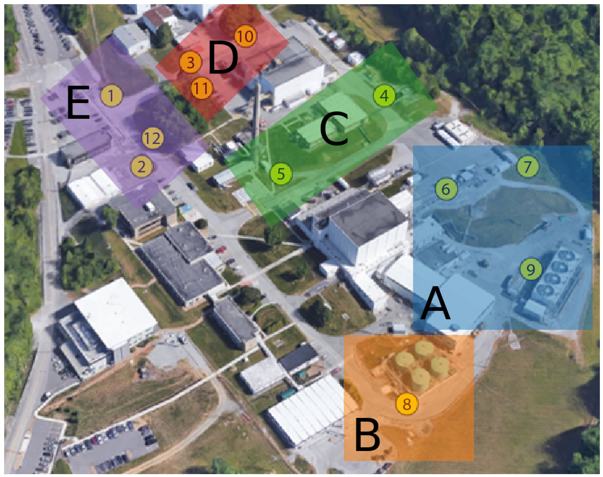
Figure 1. Overhead image of the High Flux Isotope Reactor complex at Oak Ridge National Laboratory. Multisensor platforms are mounted at the locations indicated by the yellow circles; the node ID for each platform is denoted by the circumscribed number. Regions are shaded and identified by letter with bounding boxes to provide a visual cue. Regions A, B, C, D, and E include the reactor building and cooling tower, liquid storage tanks, offices near the Radiochemical Engineering Development Center, target processing facility, and main entrance to the complex, respectively.
Jne 03 00014 g001
Figure 2. Digital mockup of the Merlyn multisensor platform and weatherproof enclosure.
Jne 03 00014 g002
Figure 3. Reactor operational state of HFIR during the 40-week data collection period.
Jne 03 00014 g003
Figure 4. Nested train–test split over the 40-week time series. The time series was partitioned into four segments, and three temporal splits were constructed using walk-forward validation and an expanding window. A one-week buffer was maintained between the test and train sets.
Jne 03 00014 g004
Figure 5. True reactor operational state (blue line) and that predicted by the baseline HMM (orange data points) for each of the three test set partitions. For Partition 1, the HMM predicted “reactor on” for all inputs. The model achieved an average accuracy across the three test partitions of 0.583.
Jne 03 00014 g005
Figure 6. True operational state (blue line) of the reactor and that predicted by the baseline feed-forward neural network (orange data points) for each of the three test set partitions. The model achieved an average accuracy across the three test partitions of 0.811 ± 0.005.
Jne 03 00014 g006
Figure 7. LONO analysis applied to the HMM. Nodes are sorted from most (top) to least (bottom) important. While most nodes have a moderate impact on model accuracy, Node 9 stands out as the most important to the classification problem and Node 2 as significantly confounding.
Jne 03 00014 g007
Figure 8. LORO analysis applied to the HMM. Regions are sorted from most (top) to least (bottom) important. Region A was identified as having a strong positive impact on model accuracy, whereas Regions E and C were identified as having negative impacts on model accuracy.
Jne 03 00014 g008
Figure 9. FNS analysis applied to the HMM. Nodes are arranged left to right in order of decreasing importance. After information was added from three nodes, additional nodes provided negative contributions to model accuracy.
Jne 03 00014 g009
Figure 10. FRS analysis applied to the HMM. Regions are arranged left to right in order of decreasing importance. After information was added from three regions, the inclusion of data from additional regions decreased model accuracy.
Jne 03 00014 g010
Figure 11. True reactor operational state (blue line) and that predicted by the HMM (green data points) using only data from the three most important nodes identified by the FNS algorithm (i.e., Nodes 1, 6, and 9). The model achieved an average accuracy across the three test partitions of 0.839, representing a significant improvement over baseline performance.
Jne 03 00014 g011
Figure 12. LONO analysis applied to the feed-forward neural network. Nodes are sorted from most (top) to least (bottom) important. Nodes 6 and 9 were identified as having positive impacts on model accuracy whereas Node 7 had a strong negative impact on model accuracy.
Jne 03 00014 g012
Figure 13. LORO analysis applied to the feed-forward neural network. Regions are sorted from most (top) to least (bottom) important. Region A demonstrated a strong positive impact on model accuracy.
Jne 03 00014 g013
Figure 14. FNS analysis applied to the feed-forward neural network. Nodes are arranged left to right in order of decreasing importance. After information was added from seven nodes, the inclusion of data from additional nodes decreased model accuracy.
Jne 03 00014 g014
Figure 15. FRS analysis applied to the feed-forward neural network. Regions are arranged left to right in order of decreasing importance. Region A was identified as most important to the classification problem.
Jne 03 00014 g015
Figure 16. True reactor operational state (blue line) and that predicted by the feed-forward neural network (green data points) using data from only the seven most important nodes, as identified using the FNS algorithm. A marginal improvement in classification performance was achieved relative to the baseline model.
Jne 03 00014 g016
Table 1. Region Descriptions.
RegionNodesDescription
A6, 7, 9Reactor Building and Cooling Tower
B8Liquid Storage Tanks
C4, 5Offices near the REDC Facility
D3, 10, 11Target Processing Facility
E1, 2, 12Main Entrance to Complex
Table 2. Merlyn sensors used for modeling.
ModalitySensor
Acceleration (3-axis)Kionix KX-224-1053 [20]
Ambient LightROHM RPR-0521RS [21]
Magnetic Field (3-axis)ROHM 1422AGMV [22]
Pressure (Barometric)ROHM BM1383AGLV [23]
TemperatureROHM BD1020HFV [24]
Table 3. Candidate scores from the first iteration of FRS analysis.
RegionAccuracy
A 0.795 ± 0.002
B 0.556 ± 0.007
C 0.500 ± 0.002
D 0.478 ± 0.002
E 0.586 ± 0.006
Table 4. Average Gini importances for Node 9 features in a decision tree model, ranked from most to least important.
Node 9 FeatureAverage Gini Importance
Magnetic Field Variance0.639
Acceleration Mean0.145
Pressure Mean0.107
Acceleration Variance0.052
Magnetic Field Mean0.020
Pressure Variance0.012
Ambient Light Mean0.005
Ambient Light Variance0.005
Temperature Mean0.005
Temperature Variance0.003
Missing Flag0.002
Publisher’s Note: MDPI stays neutral with regard to jurisdictional claims in published maps and institutional affiliations.

