2. Mathematical Framework of the 1st-Casam for Operator-Valued Responses of Coupled Systems Comprising Imprecisely Known Parameters, Interfaces and Boundaries
The system considered in this work comprises two nonlinear sub-systems which are coupled to one another across a common internal interface (boundary) in phase–space, and which will be called “Subsystem I” and, respectively, “Subsystem II”. The first subsystem is represented mathematically as follows:
Bold letters will be used in this work to denote matrices and vectors. Unless explicitly stated otherwise, the vectors in this work are considered to be column vectors. The second subsystem is represented mathematically as follows:
If differential operators appear in Equations (1) and (2), a corresponding set of boundary and/or initial/final conditions must also be given, these conditions can be represented in operator form as follows:
The quantities appearing in Equations (1)–(3) are defined as follows:
denotes a column vector having scalar-valued components representing all of the imprecisely known internal and boundary parameters of the physical systems, including imprecisely known parameters that characterize the interface and boundary conditions. Some of these parameters are common to both physical systems, e.g., the parameters that characterize common interfaces. These scalar parameters are considered to be subject to both random and systematic uncertainties, as is usually the case in practical applications. In order to use such parameters in practical computations, which is the scope of the methodology presented in this work, they are considered to be either “uncertain” or “imprecisely known”. “Uncertain” parameters are usually considered to follow a probability distribution having a known “mean value” and a known “standard deviation”. On the other hand, the actual values of “imperfectly known” parameters are unknown. To enable the use of such parameters in computations, “expert opinion” is invoked to assign each of such imprecisely known parameters a “nominal value” (which plays the role of a “mean value”) and a “range of variation” (which plays the role of a standard deviation). For practical computations, the actual origin of the parameter’s nominal (or mean) value and of its assigned standard deviation is immaterial, which is why the qualifiers “uncertain” and “imprecisely known” are often used interchangeably. In this work, the superscript “zero” will be used to denote the known nominal or mean values of various quantities. In particular, the vector of nominal and/or mean parameter values will be denoted as . The symbol “” will be used to denote “is defined as” or “is by definition equal to” and transposition will be indicated by a dagger superscript.
denotes the phase–space position vector, of dimension , of independent variables for the system defined in Equation (1). The vector of independent variable is defined on a phase–space domain denoted as , , and is therefore considered to depend on the uncertain parameters . The lower-valued imprecisely known boundary-point of the independent variable is denoted as , while the upper-valued imprecisely known boundary-point of the independent variable is denoted as . For physical systems modeled by diffusion theory, for example, the “vacuum boundary condition” requires that the particle flux vanish at the “extrapolated boundary” of the spatial domain facing the vacuum; the “extrapolated boundary” depends on the imprecisely known geometrical dimensions of the system’s domain in space and also on the system’s microscopic transport cross sections and atomic number densities. The boundary of the domain comprises all of the endpoints and of the intervals on which the respective components of are defined. It may happen that some components and/or are infinite, in which case they would not depend on any imprecisely known parameters.
denotes a -dimensional column vector whose components represent the system’s dependent variables (also called “state functions”). The vector-valued function is considered the unique nontrivial solution of the physical problem described by Equations (1) and (3).
denotes a column vector of dimensions whose components are operators that act nonlinearly on and .
denotes a -dimensional column vector whose elements represent inhomogeneous source terms that depend either linearly or nonlinearly on . The components of may involve operators (rather than just finite-dimensional functions) and distributions acting on and .
denotes the -dimensional phase–space position vector of independent variables for the physical system defined in Equation (2). The vector of independent variable is defined on a phase–space domain denoted as , which is defined as follows: . The lower-valued imprecisely known boundary-point of the independent variable is denoted as , while the upper-valued imprecisely known boundary-point of the independent variable is denoted as . Some or all of the points may coincide with the points . Additionally, some components of may coincide with some components of , in which case the respective lower and upper boundary points for the respective coinciding independent variables would also coincide correspondingly. The boundary of the domain comprises all of the endpoints and of the intervals on which the respective components of are defined.
denotes a -dimensional column vector whose components represent the system’s dependent variables (also called “state functions”). The vector-valued function is considered the unique nontrivial solution of the physical problem described by Equations (2) and (3).
denotes a column vector of dimensions whose components are operators acting nonlinearly on and .
denotes a -dimensional column vector whose elements represent inhomogeneous source terms that depend either linearly or nonlinearly on . The components of may involve operators and distributions acting on and .
The vector-valued operator comprises all of the boundary, interface, and initial/final conditions for the coupled physical systems. If the boundary, interface and/or initial/final conditions are inhomogeneous, which is most often the case, then .
Since and may involve operators and distributions acting on and , all of the equalities in this work, including Equations (1)–(3), are considered to hold in the weak (“distributional”) sense.
The nominal (or “base-case”) solutions of Equations (1)–(3), denoted as
and
, are obtained by solving these equations at the nominal parameter values
, i.e.,
The response considered in this work is a generic nonlinear function-valued operator, denoted as follows:
The nominal value of the response, denoted as , is determined by computing the response at the nominal values , and . The true values of imprecisely known model, interface and boundary parameters may differ from their nominal (average, or “base-case”) values by variations denoted as , where , . In turn, the parameter variations will cause variations and in the state functions and all of these variations will cause variations in the response around the nominal response value . Sensitivity analysis aims at computing the functional derivatives (called “sensitivities”) of the response to the imprecisely known parameters . Subsequently, these sensitivities can be used for a variety of purposes, including quantifying the uncertainties induced in responses by the uncertainties in the model and boundary parameters, combining the uncertainties in computed responses with uncertainties in measured response (“data assimilation”) to obtain more accurate predictions of responses and/or parameters (“model calibration”, “predictive modeling”, etc.).
As has been shown by Cacuci [
1], the most general definition of the 1st-order total sensitivity of an operator-valued model response to parameter variations is provided by the first-order “Gateaux-variation” (G-variation) of the response under consideration. To determine the first G-variation of the response
, it is convenient to denote the functions appearing in the argument of the response as being the components of a vector
, which represents an arbitrary “point” in the combined phase–space of the state functions and parameters. The point which corresponds to the nominal values of the state functions and parameters in this phase space is denoted as
. Analogously, it is convenient to consider the variations in the model’s state functions and parameters to be the components of a “vector of variations”,
, defined as follows:
. The 1st-order Gateaux- (G-) variation of the response
, which will be denoted as
, for arbitrary variations
in the model parameters and state functions in a neighborhood
around
, is obtained, by definition, as follows:
The unknown variations
and
in the state functions are related to the variations
through the equations obtained by applying the definition of the G-differential to the equations underlying the coupled nonlinear, i.e., Equations (1)–(3), to obtain the following relations:
Performing in Equations (9)–(11) the differentiations with respect to
and setting
in the resulting expression yields the following system of equations:
The system of equations comprising Equations (12)–(14) is called the “First-Level Forward Sensitivity System” (1st-LFSS) and could be solved to obtain the variations and in the state functions in terms of the parameter variations which appear as sources in the 1st-LFSS equations. Subsequently, the variations and thus obtained could be used to compute the total sensitivity defined in Equation (8).
The existence of the G-variations of the operators underlying the 1st-LFSS and total sensitivity
does not guarantee their numerical computability. Numerical methods most often require that
and the operators underlying the 1st-LFSS be linear in the variations
in a neighborhood
around
. The necessary and sufficient conditions for the G-differential
of a nonlinear operator
to be linear in
in a neighborhood
around
, and thus admit partial and total G-derivatives, are as follows [
6]:
- (i)
satisfies a weak Lipschitz condition at
;
- (ii)
for two arbitrary vectors of variations
and
, the operator
satisfies the following relation:
It will henceforth be assumed that the operators
,
,
,
,
and
satisfy the conditions indicated in Equations (15) and (16). Hence, Equations (12)–(14) can be written in the following form:
where
The partial G-derivatives
,
,
,
,
,
,
,
and
, which appear in Equations (17)–(21), are matrices of corresponding dimensions. When the G-variation
is linear in
, it is called the G-differential of
and is usually denoted as
. Furthermore, the result of the differentiations indicated on the right-side of the definition provided in Equation (8) can be written as follows:
where the so-called “direct-effect” term is defined as follows:
while the so-called “indirect-effect” term is defined as follows:
In Equations (23) and (24), the vectors , and comprise, as components, the first-order partial G-derivatives computed at the phase–space point . The G-differential is an operator defined on the same domain as and has the same range as . The G-differential satisfies the relation with .
The “direct effect” term
depends only on the parameter variations
so it can be computed immediately, since it does not depend on the variations
and
. On the other hand, “indirect effect” term
depends indirectly on the parameter variations
through the yet unknown variations
and
in the state functions, and these functions can be determined only by solving repeatedly the 1st-LFSS for every possible parameter variation
. The need for these prohibitively expensive computations can be circumvented by extending the concepts underlying the “Adjoint Sensitivity Analysis Methodology” (ASAM) conceived by Cacuci [
1] to construct a “First-Level Adjoint Sensitivity System” (1st-LASS), the solution of which will be independent of the variations
,
and
. Subsequently, the solution of the 1st-LASS will be used to compute the indirect-effect term
by constructing an equivalent expression (for this indirect-effect term) which would not involve the unknown variations
and
.
2.1. Spectral Representation of the System Response’s Indirect-Effect Term
Since the indirect-effect term
is defined on the same domain
as
, and has the same range as
, it follows that it can be represented in the following form:
where
and
The following designations have been used in Equations (26) and (27): (i) the quantities , , denote the corresponding spectral basis functions (e.g., orthogonal polynomials, Fourier exponential/trigonometric functions) for the domain defined as the domain ; (ii) the quantities , , denote the spectral functions corresponding to the domain ; and (iii) the quantities and denote the corresponding generalized spectral (Fourier) coefficients.
The appearance of the “difficult to compute” variations and in the functionals defined in Equations (26) and (27), respectively, can be eliminated by expressing the right-sides of Equations (26) and (27) in terms of adjoint functions that will be obtained by implementing the following sequence of steps:
Introduce a Hilbert space pertaining to the domain , denoted as , comprising square-integrable vector-valued elements of the form and , where , , , .
Define the inner product, denoted as
, between two elements of
, as follows:
where
and
Recast Equations (17) and (18) in the following matrix from:
Use the definition provided in Equation (28) to form the inner product of Equation (31) with a square-integrable vector
to obtain the following relation:
Using the definition of the adjoint operator in the Hilbert space
, recast the left-side of Equation (32) as follows:
where the operator
denotes the formal adjoint of
, the operator
denotes the formal adjoint of
and where
denotes the bilinear concomitant evaluated on the boundary
. The superscript “1” which appears in the notation of the bilinear concomitant
indicates that this quantity arises in conjunction with the construction of the “First-Level Adjoint Sensitivity System (1st-LASS)”.
Replace the left-side of Equation (33) with the right-side of Equation (32) to obtain the following relation:
Require the left-side of Equation (34) to represent the indirect-effect term
defined in Equation (25), which can be fulfilled by requiring the yet undetermined (adjoint) functions
and
to satisfy the following equations:
Since the source terms on the right-sides of Equations (35) and (36) depend on the indices of the spectral bases functions, it follows that the adjoint functions and also depend on the respective indices, which will henceforth be explicitly displayed by writing and , respectively.
The boundary, interface, and initial/final conditions for the functions and are now determined by imposing the following requirements:
- (a)
Implement the boundary, interface and initial/final conditions given in Equation (19) into the bilinear concomitant in Equation (34).
- (b)
Eliminate the remaining unknown boundary, interface and initial/final conditions involving the functions
and
from the expression of the bilinear concomitant in Equation (34) by selecting boundary, interface and initial/final conditions for the adjoint functions
and
such that the selected conditions for these adjoint functions must be independent of unknown values of
,
and
while ensuring that Equations (35) and (36) are well posed. The boundary conditions thus chosen for the adjoint functions
and
can be represented in operator form as follows:
where the subscript “
A” indicates “adjoint” and the superscript “1” indicates that these boundary conditions arises in conjunction with the construction of 1st-LASS. The selection of the boundary conditions for the adjoint functions
and
represented by Equation (37) eliminates the appearance of any unknown values of the variations
and
in the bilinear concomitant in Equation (34), reducing it to a residual quantity that contains boundary terms involving only known values of
,
,
,
,
, and
. This residual bilinear concomitant will be denoted as
.
In general, this residual bilinear concomitant does not automatically vanish, although it may do so in particular instances. In principle, this residual bilinear concomitant could be forced to vanish, if necessary, by considering extensions, in the operator sense, of the linear operators and/or , but such extensions seldom need to be used in practice.
Using Equations (34)–(36) in conjunction with Equations (26) and (27) in Equation (25) yields the following expression for the indirect-effect term
:
As the expression in Equation (38) indicates, the desired elimination from of the unknown variations and has been accomplished by having replaced them by the adjoint functions and , which do not depend on any parameter variations; this fact that has been underscored by having explicitly indicated that the indirect-effect term can now be written in the form .
When first introduced in Equation (32), it was not known that the adjoint functions would ultimately depend on the indices
and
; this fact has become apparent only after having constructed the right-sides (i.e., sources) of Equations (35) and(36) to emphasize this fact. These equations are re-written below:
The system of Equations (39) and (40), together with the adjoint boundary/initial conditions represented by Equation (37) will be called the “First-Level Adjoint Sensitivity System (1st-LASS).” The 1st-LASS is independent of the parameter variations but depends on the indices and . In principle, therefore, the 1st-LASS needs to be solved as many times as there are nonzero spectral basis functions, which act as sources on the right side of the equations underlying the 1st-LASS. It is therefore very important to represent the indirect-effect term defined in Equation (25) using as few basis-functions as possible, within a criterion of accuracy that is set by the user, a priori. Once the adjoint functions and are available, they can be used in Equation (38) to compute the indirect-effect term exactly and efficiently, using quadrature formulas, which are many orders of magnitude faster to compute than solving the operator (differential, integral) equations that underlie the 1st-LFSS.
In practice, orthogonal polynomials will often be selected to serve as basis-functions for the spectral Fourier representations of the responses of interest. As is well-known, orthogonal polynomials possess many recurrence relations which can be advantageously used to reduce massively the number of computations that would actually require solving the 1st-LASS.
In the particular case when the response is a scalar-valued functional of the system’s dependent variables, the expansion in Equation (25) reduces to a single term, so that the summations in the expression of the indirect-effect term in Equation (38) also reduce to a single term.
2.2. Pseudo-Spectral Representation of the System Response’s Indirect-Effect Term
Alternatively, Lagrange interpolation, see e.g., [
7], can be used to express the indirect-effect term defined in Equation (24) approximately as follows:
where the quantities
represent the “cardinal functions”, where
and
denote the collocation (or interpolation) points, and where
The cardinal functions
are also called [
3] the “fundamental polynomials for pointwise interpolation”, the “elements of the cardinal basis”, the “Lagrange basis”, or the “shape functions”. Depending on the domains of definition
and choices of weight functions, particularly important cardinal functions are the Chebyshev, Legendre, Gegenbauer, Hermite, Laguerre polynomials, and Whittaker’s “sinc” function. In several dimensions, it is most efficient to use a tensor product basis, i.e., use basis functions that are products of one-dimensional basis functions. Particularly efficient computational procedures can be constructed when both the basis functions and grid are tensor products of one-dimensional functions and grids, respectively. Using trigonometric functions, Chebyshev polynomials, or rational Chebyshev functions as basis functions enables the use of the Fast Fourier Transform, which further enhances computational efficiency.
Following established practice [
3], “collocation points” and “interpolation points” will be used as synonyms in this work, as will be the terms “collocation” and “pseudospectral” when referring to the fact that interpolatory methods will be used to determine the yet unknown indirect-effect term
by expressing it in terms of adjoint functions specifically developed for each of the collocation/interpolation points. The reason that “collocation” methods are alternatively labeled “pseudospectral” is that the optimum choice of the interpolation points makes collocation methods identical with the Galerkin method if the inner products are evaluated by “Gaussian integration”. It is important to note that neither the cardinal functions
nor the collocation points
and
are subject to model parameter uncertainties.
The functionals
defined in Equation (42) can be evaluated by using adjoint functions that are the solutions of a 1st-LASS constructed by following the same conceptual steps as those leading to Equations (39) and (40), and the adjoint boundary conditions defined by Equation (37). Omitting these intermediate steps, the final result is as follows:
where the adjoint functions
and
are the solutions of the following 1st-LASS:
It is evident from Equations (44)–(46) that the 1st-LASS must be solved anew for each of the collocation/interpolation points considered in the expansion of the indirect-effect term shown in Equation (41). The choice between using the spectral expansion shown in Equation (25) or using the collocation/interpolation pseudo-spectral expansion shown in Equation (41) depends on the specific problem under consideration, but for comparable accuracy in the computation of the response sensitivities, using the collocation/interpolation pseudo-spectral expansion shown in Equation (41) is often more efficient computationally than using the full spectral expansion.
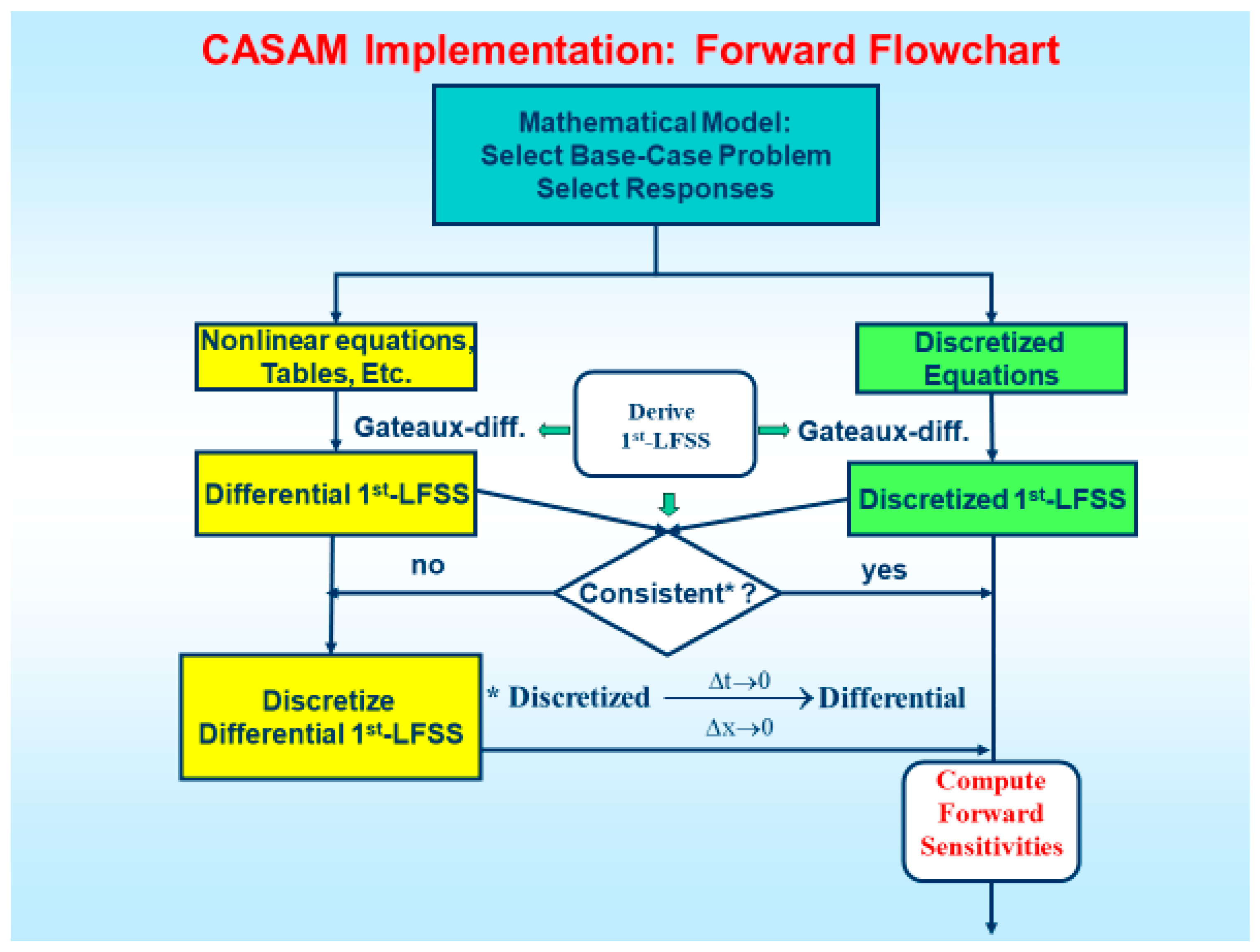
The practical implementation of the mathematical methodology underlying the 1st-CASAM is illustrated in
Figure 1 and
Figure 2. The derivation of the 1st-LFSS is illustrated in
Figure 1. The path on the left side of
Figure 1 depicts the derivation of the (non-discretized) 1st-LFSS starting from the differential equations underlying the original nonlinear system. On the other hand, the path on the right-side of
Figure 1 depicts the derivation of the discretized 1st-LFSS starting from the discretized form of the original nonlinear equations. If this path is followed, it must be ensured that the discretized 1st-LFSS is consistent with the differential form of the 1st-LFSS in the limit of vanishing size of the discretization interval considered for the independent variables.
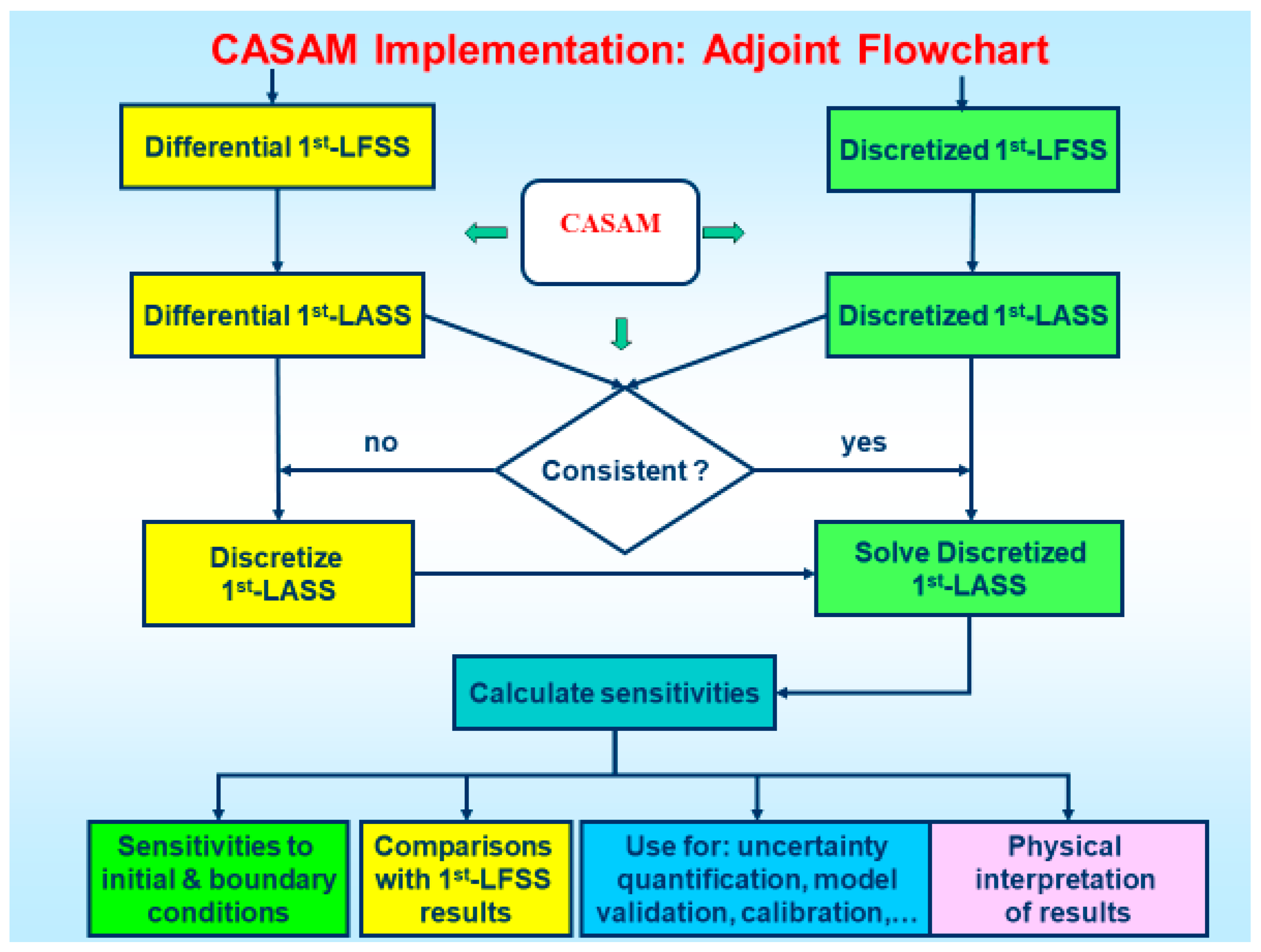
The derivation of the 1st-LASS is illustrated in
Figure 2. The path on the left side of
Figure 2 depicts the derivation of the (non-discretized) 1st-LASS starting from the differential form of the 1st-LFSS. On the other hand, the path on the right side of
Figure 2 depicts the derivation of the discretized 1st-LASS starting from the discretized 1st-LFSS. If this path is chosen, the consistency of the discretized 1st-LASS with the differential form of the 1st-LFSS must again be ensured.
3. Concluding Remarks
This work has presented the First-Order Comprehensive Adjoint Sensitivity Analysis Methodology (1st-CASAM) for computing efficiently the exact first-order sensitivities (i.e., functional derivatives) of operator-valued responses (i.e., model results) of general models of coupled nonlinear physical systems characterized by imprecisely known parameters, internal interfaces between the coupled systems and external boundaries. When the model response is a (scalar-valued) functional of the system’s dependent variables (i.e., state functions), the total sensitivity of a scalar-valued functional response to all of the model’s state functions is (also) a functional of the variations in the model’s state variables. By being a functional of the variations in the model’s state variables, the total response sensitivity naturally defines an inner product in terms of which it can be expressed uniquely by virtue of the well-known Riesz Representation Theorem (which ensures that every functional defined in a Hilbert space can be expressed uniquely as an inner product). The existence of such a natural inner-product induced by a functional response enables the construction of an appropriate adjoint sensitivity system, the solution of which (i.e., the respective adjoint sensitivity functions) can always be used to compute, exactly and most efficiently, the sensitivities of a functional response to the model’s scalar parameters. When the response is a functional of the state variables, a single adjoint computation (i.e., solution of the adjoint sensitivity system) suffices for subsequently computing exactly all of the model’s response sensitivities to all of the model’s scalar parameters. The adjoint sensitivity system has the same dimensions as the original system, but it is always linear in the adjoint state functions. This is in contradistinction to the original system, which is usually nonlinear in its state functions. Solving the original forward system and the adjoint sensitivity system involve large-scale computations, since these systems invariably involve inversion of large matrices stemming from differential, difference, integral, and/or algebraic equations. Since the adjoint sensitivity analysis methodology requires solving just once the adjoint sensitivity system, this methodology is the most advantageous to use computationally in practice for large-scale systems involving many parameters.
On the other hand, the total sensitivity (to model parameters and state functions) of a model response which is a function-valued (as opposed to a scalar-valued) operator of the model’s state functions does not provide a natural inner product for the model/system under consideration. Without an inner product, it is not possible to construct an adjoint sensitivity system, the solution of which would subsequently be used for computing the response sensitivities to the model’s parameters. Therefore, an inner product must first be constructed to enable expressing the operator-valued total response sensitivity to the variations in the state functions in terms of functionals of the system’s dependent variables (state functions). The requisite inner product can be constructed by representing the total sensitivity of the operator-valued response to the system’s state functions in terms of scalar-valued (functionals) response using: (i) spectral expansions; or (ii) collocation/pseudo-spectral expansions, or (iii) combined spectral/collocation expansions. The coefficients in any of these expansions are functionals that can be represented in terms of an inner product. In turn, this inner product enables the construction of an adjoint sensitivity system, the solution of which can subsequently be used to compute exactly and efficiently the sensitivities of these coefficients to the model’s parameters. A different source for the adjoint sensitivity system is developed for each spectral coefficient or for each collocation point. Altogether, therefore, as many adjoint computations would be needed as there are spectral coefficients and/or collocation points in the phase–space of independent variables. Thus, for operator-valued responses, the fundamental issue is to establish the number of collocation points in the phase–space of independent variables and/or the number of Fourier coefficients which would be needed for representing the response within an a priori established accuracy in the phase–space of independent variables. Subsequently, for each Fourier coefficient and/or at each collocation point, the 1st-CASAM provides the exact sensitivities in the parameter space, in the computationally most efficient manner. By enabling the exact computations of operator-valued response sensitivities to internal interfaces and external boundary parameters and conditions, the 1st-CASAM presented in this work makes it possible, inter alia, to quantify the effects of manufacturing tolerances on the responses of physical and engineering systems.
An accompanying work [
7] will present the application of the 1st-CASAM developed in this work to a benchmark problem [
8] that models coupled heat conduction and convection in a physical system comprising an electrically heated rod surrounded by a coolant which simulates the geometry of a nuclear reactor. In particular, this benchmark [
8] was used to verify [
8,
9] the numerical results produced by the FLUENT Adjoint Solver [
10].


