
PEMFC Thermal Management Control Strategy Based on Dual Deep Deterministic Policy Gradient


Abstract
1. Introduction
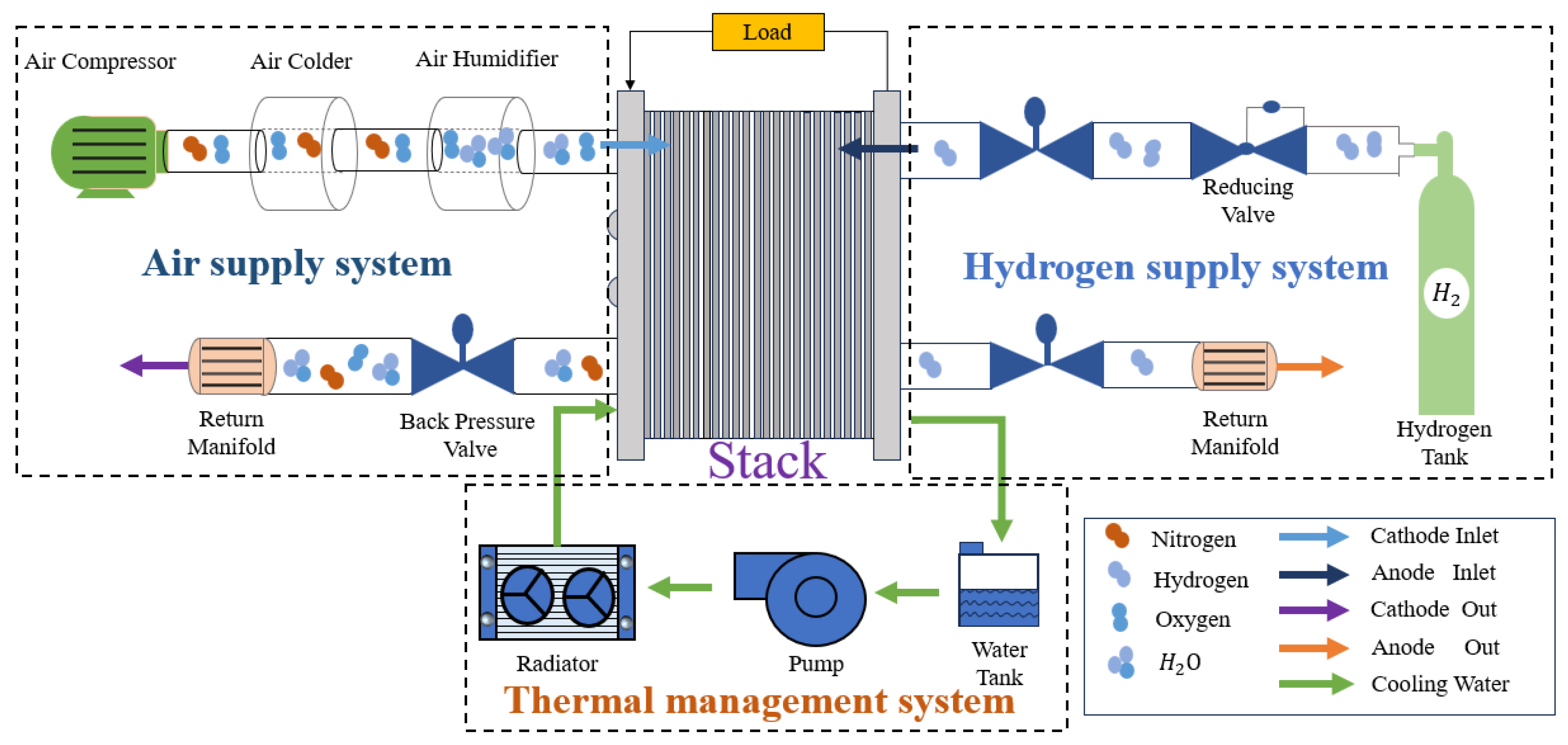
2. PEMFC System Model
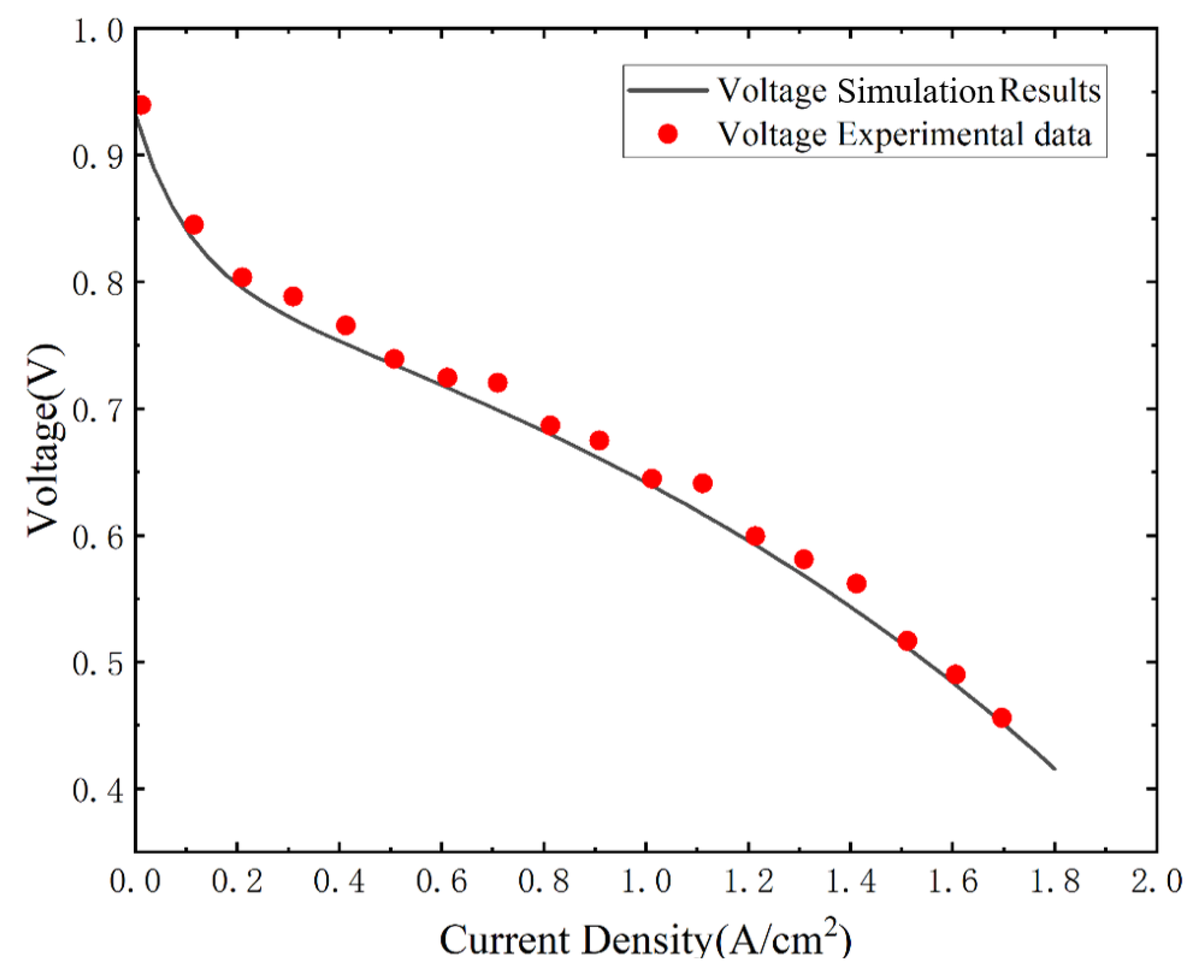
2.1. Fuel Cell Modeling
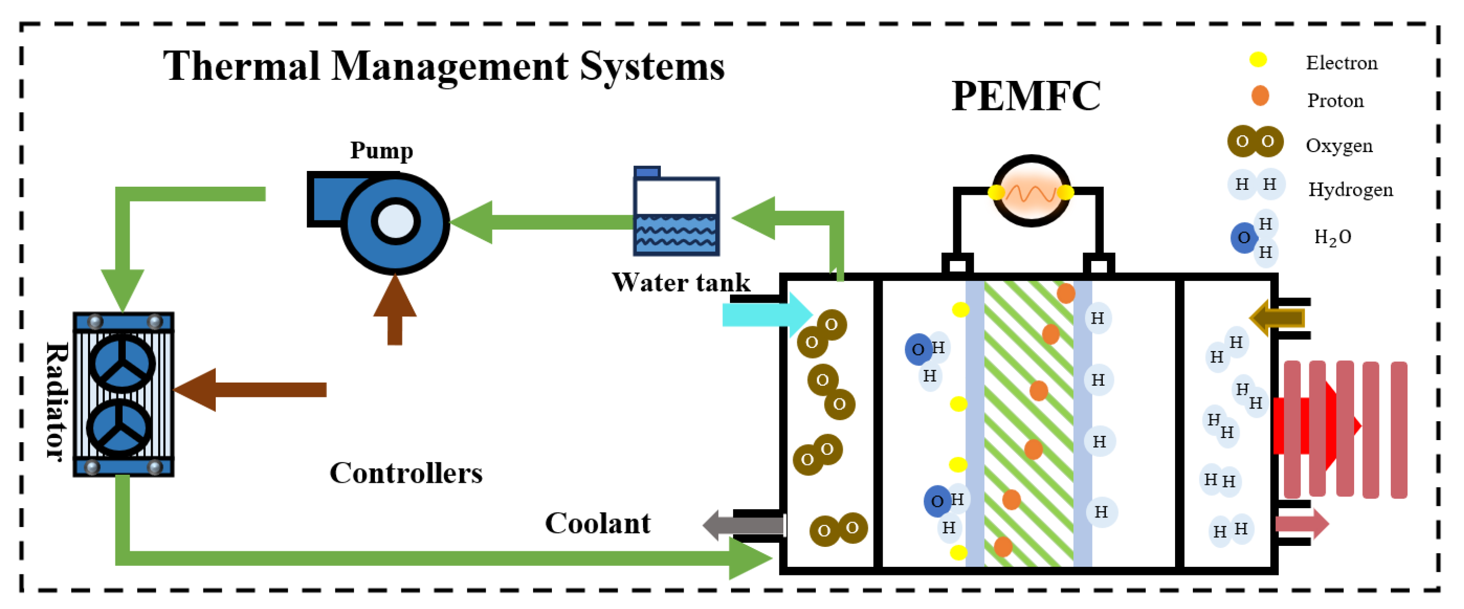
2.2. PEMFC Thermal Management System Modeling
2.2.1. PEMFC Thermal Modeling
2.2.2. Radiator Modeling
3. Deep Deterministic Policy Gradient Strategy
3.1. DDPG Algorithm Description
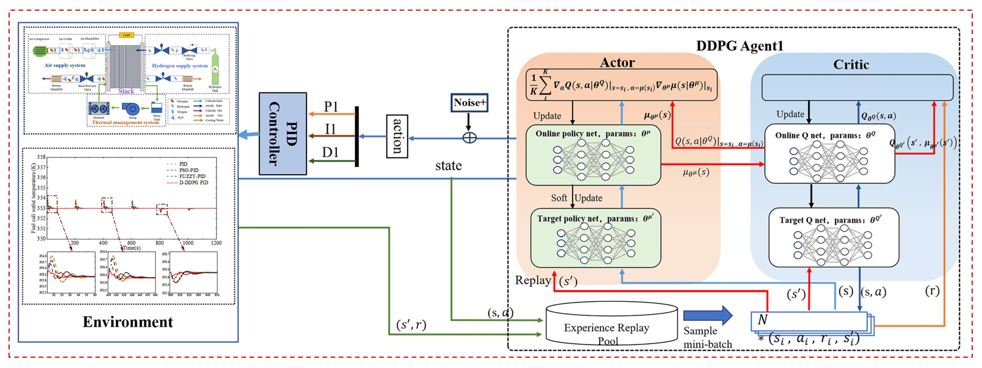
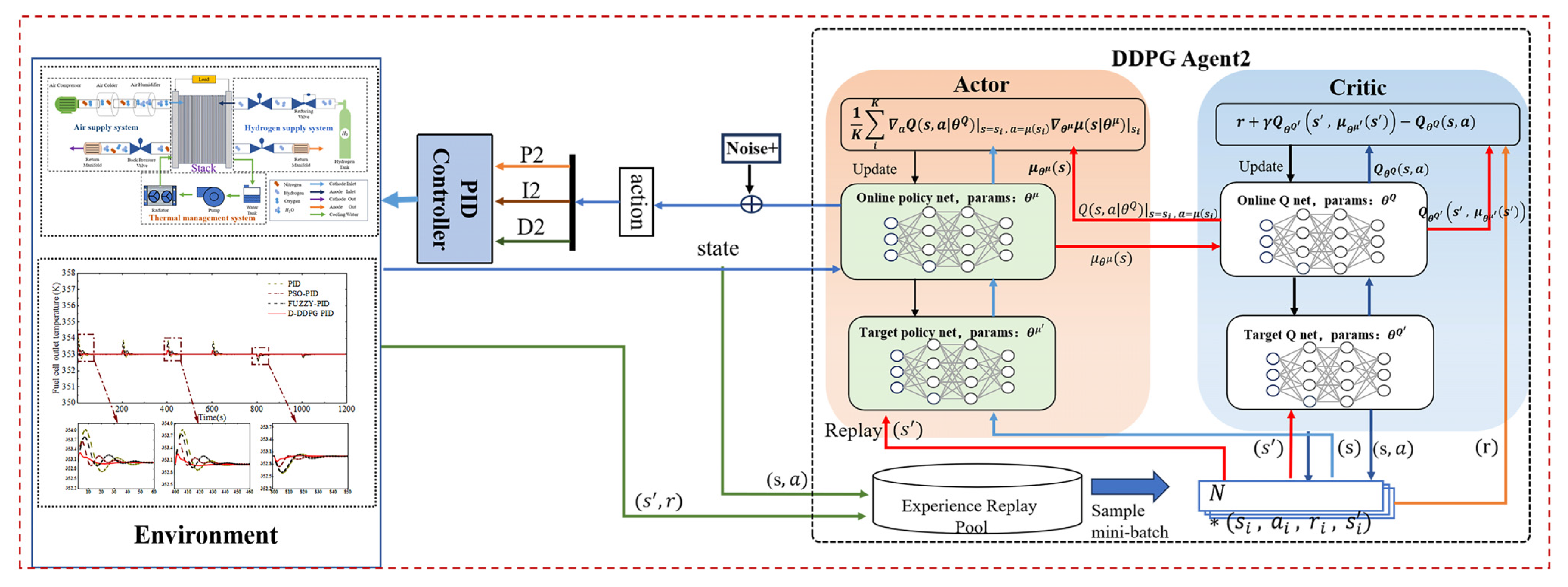
3.2. Temperature Control Architecture for PEMFC Based on Dual DDPG-PID
3.3. Details of the DDPG
3.3.1. State
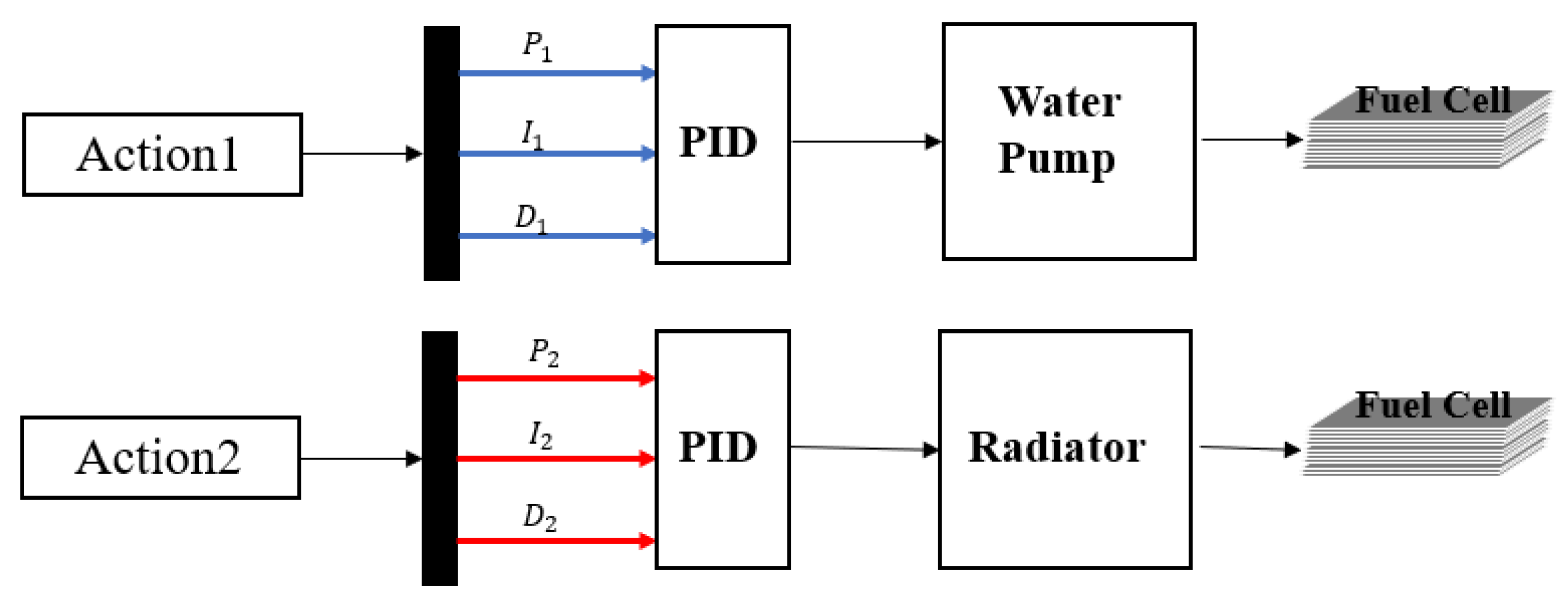
3.3.2. Action
3.3.3. Reward Function
4. The Thermal Management Strategy Based on Dual DDPG-PID
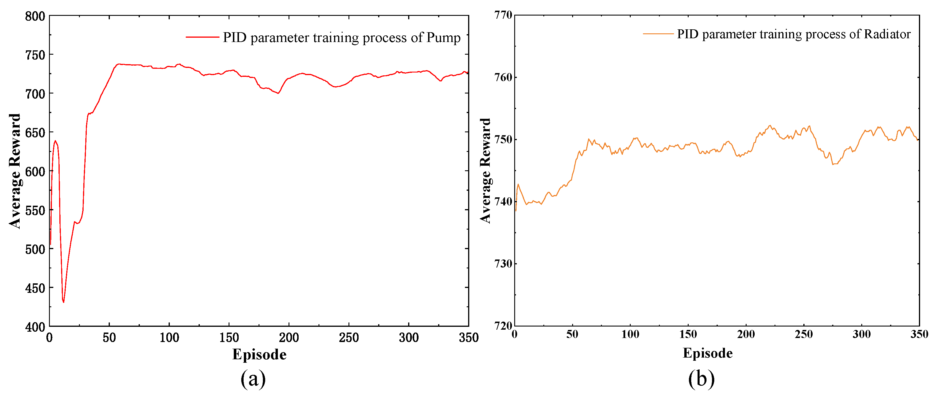
4.1. Training and Simulation Results
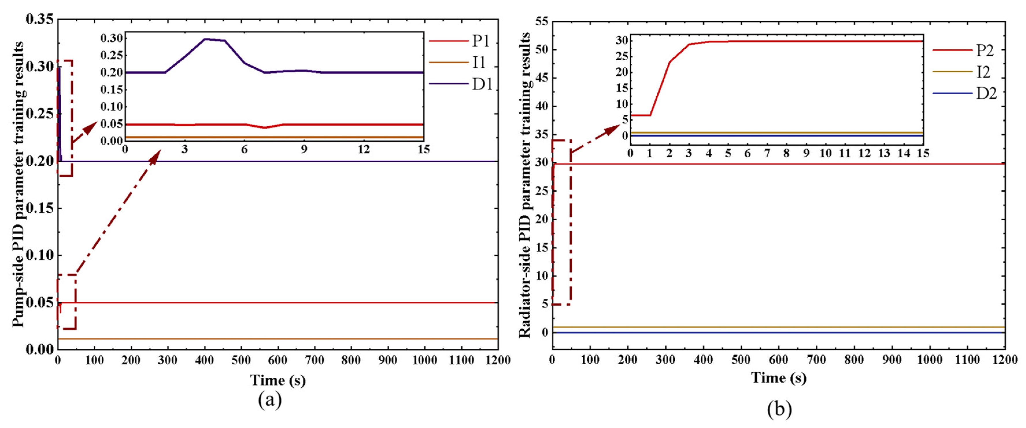
4.2. Analysis of Training Results of Dual DDPG-PID
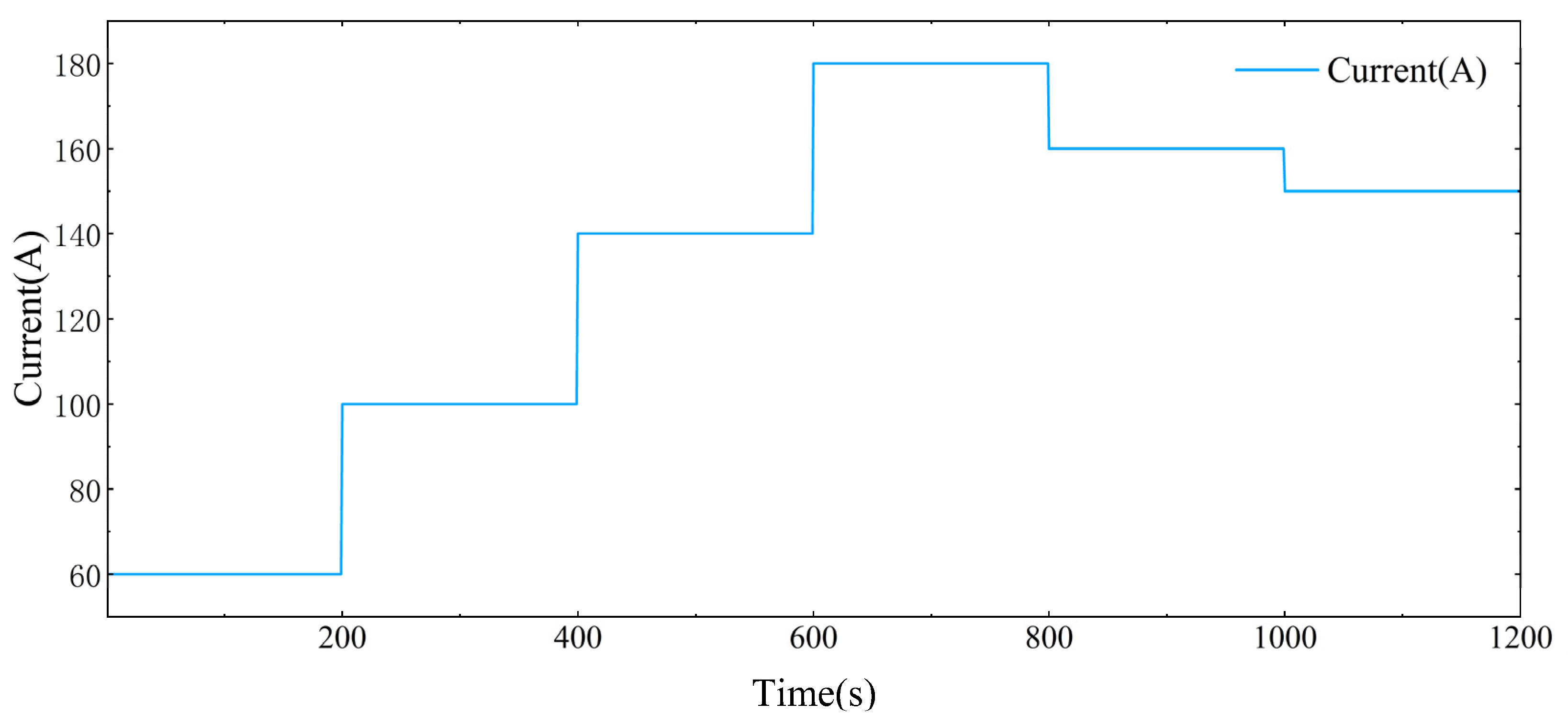
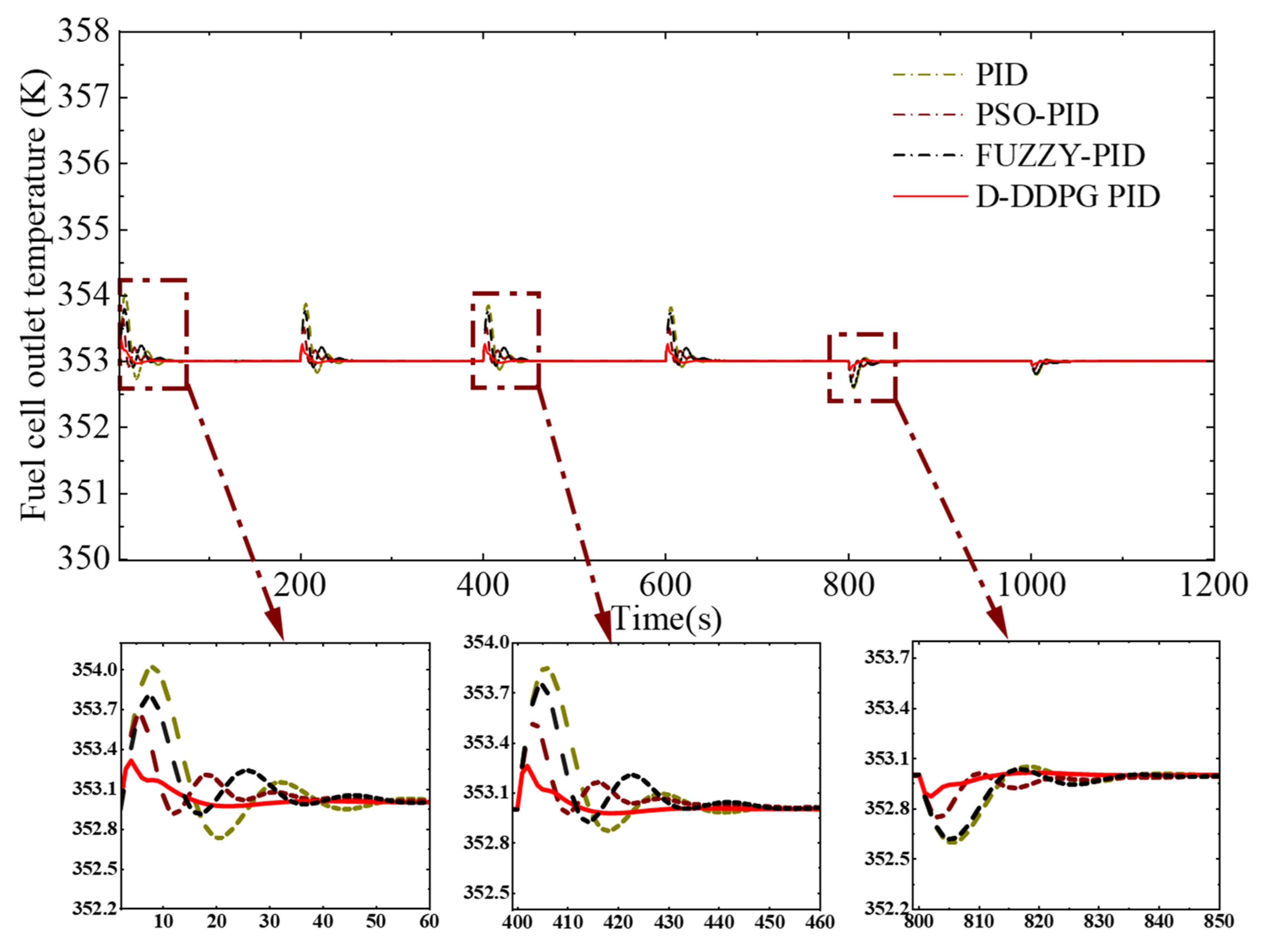
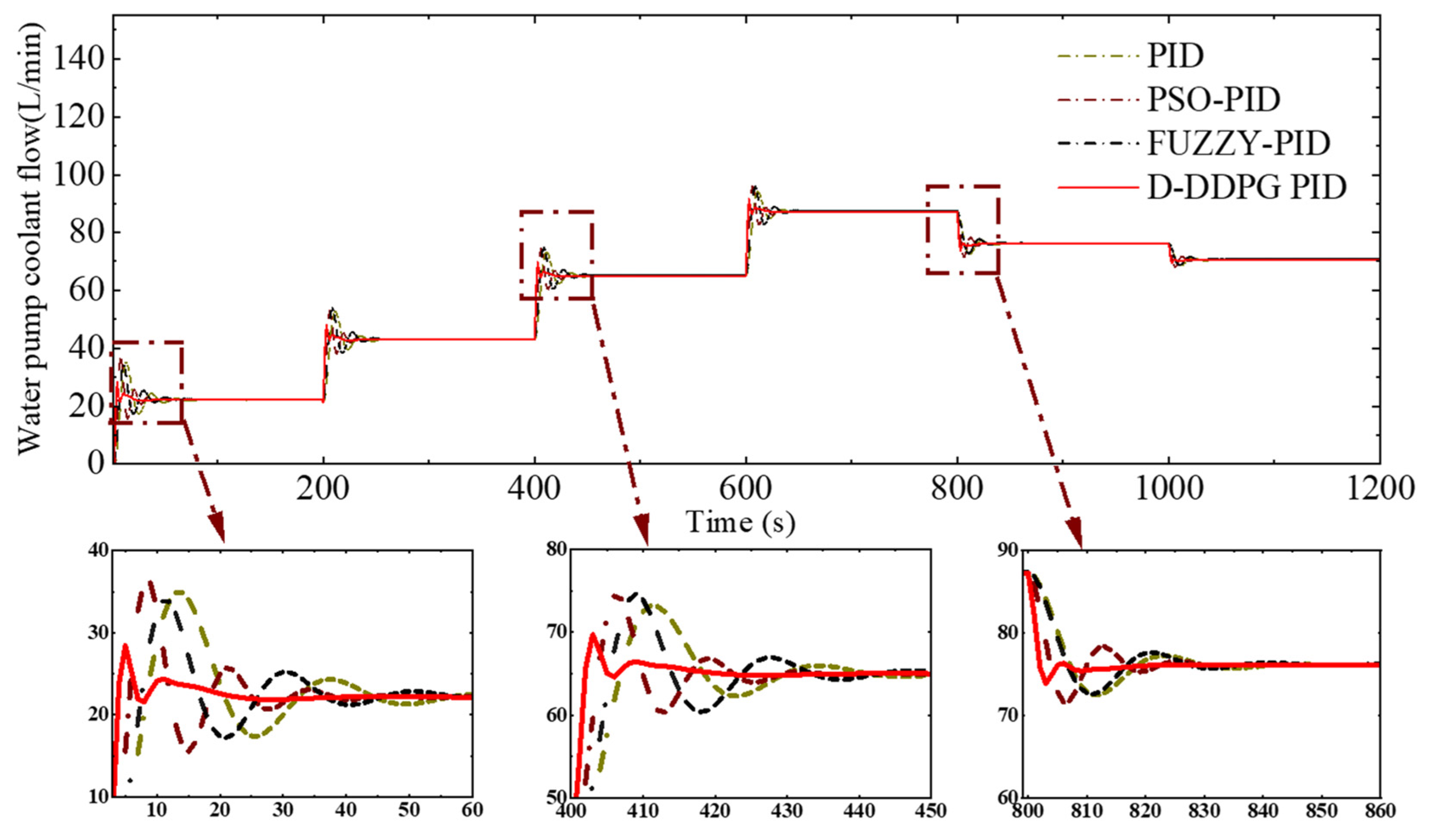
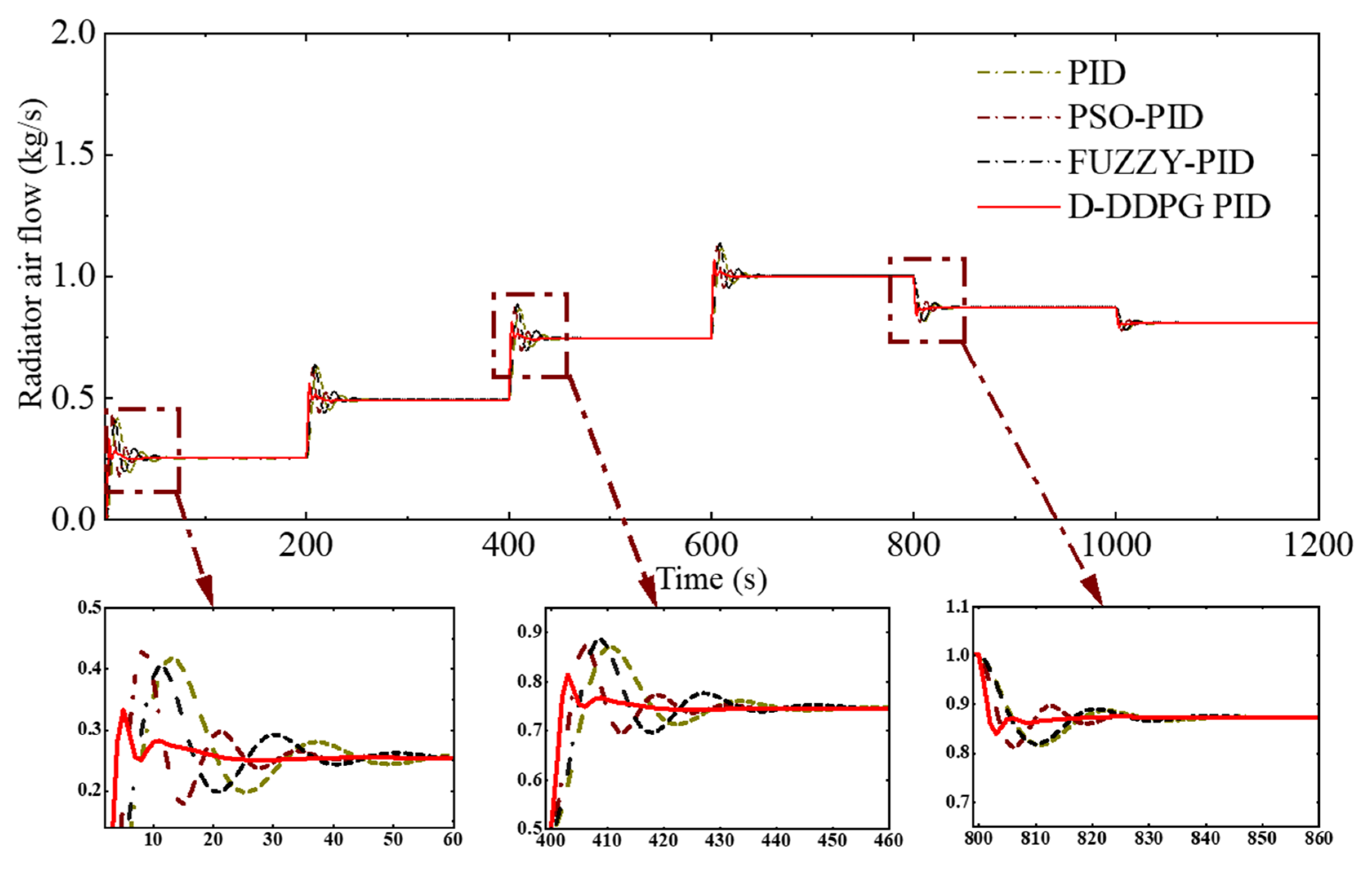
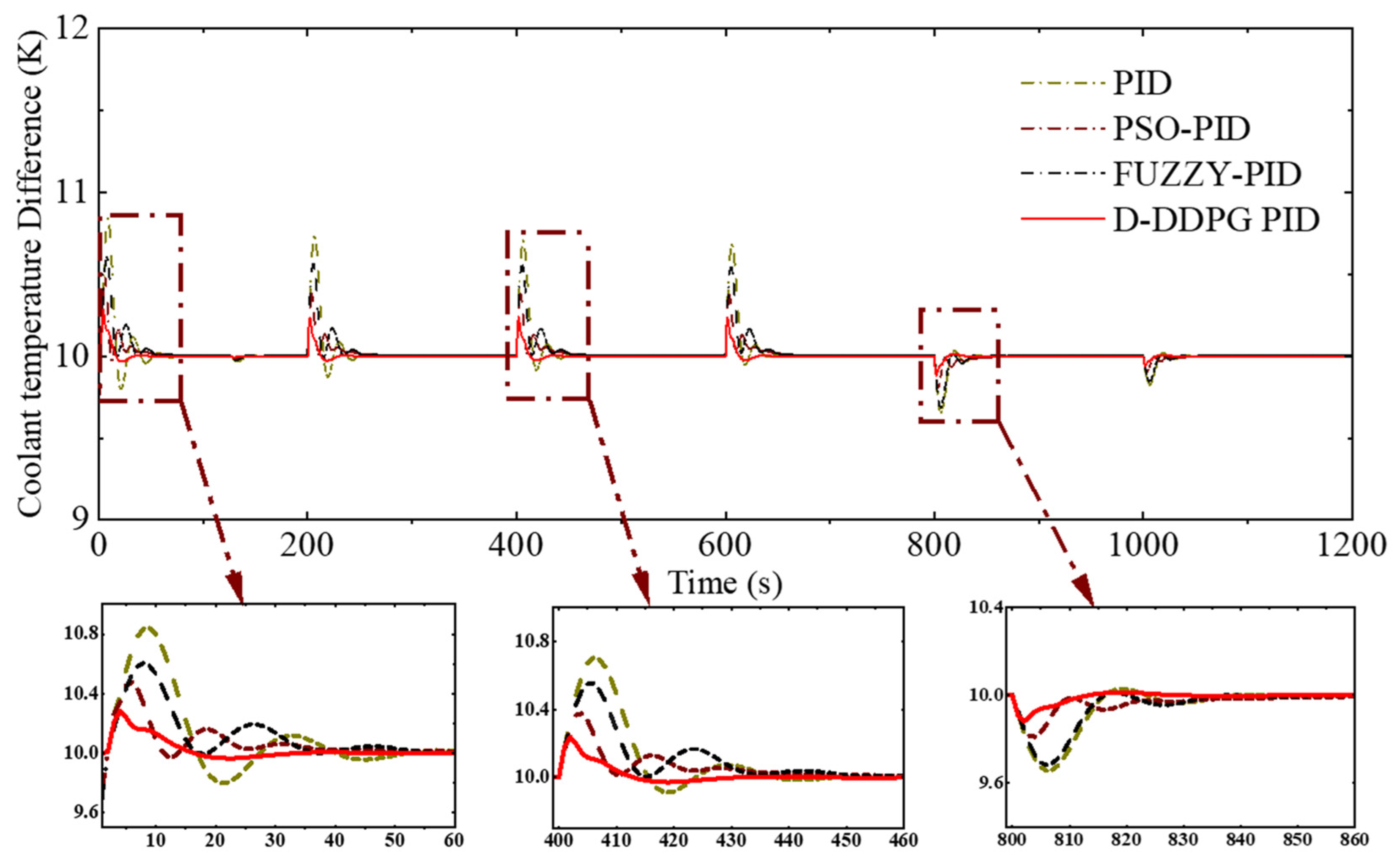
4.3. Temperature Regulation in Response to Continuous Variations in Load Current
5. Conclusions
Author Contributions
Funding
Data Availability Statement
Conflicts of Interest
Appendix A. Cathode and Anode Flow Channel Model and Membrane Water Content Model
Appendix A.1. Cathode and Anode Flow Channel Modeling
Appendix A.2. Membrane Water Content Modeling
Appendix B. PEMFC Auxiliary System Modeling
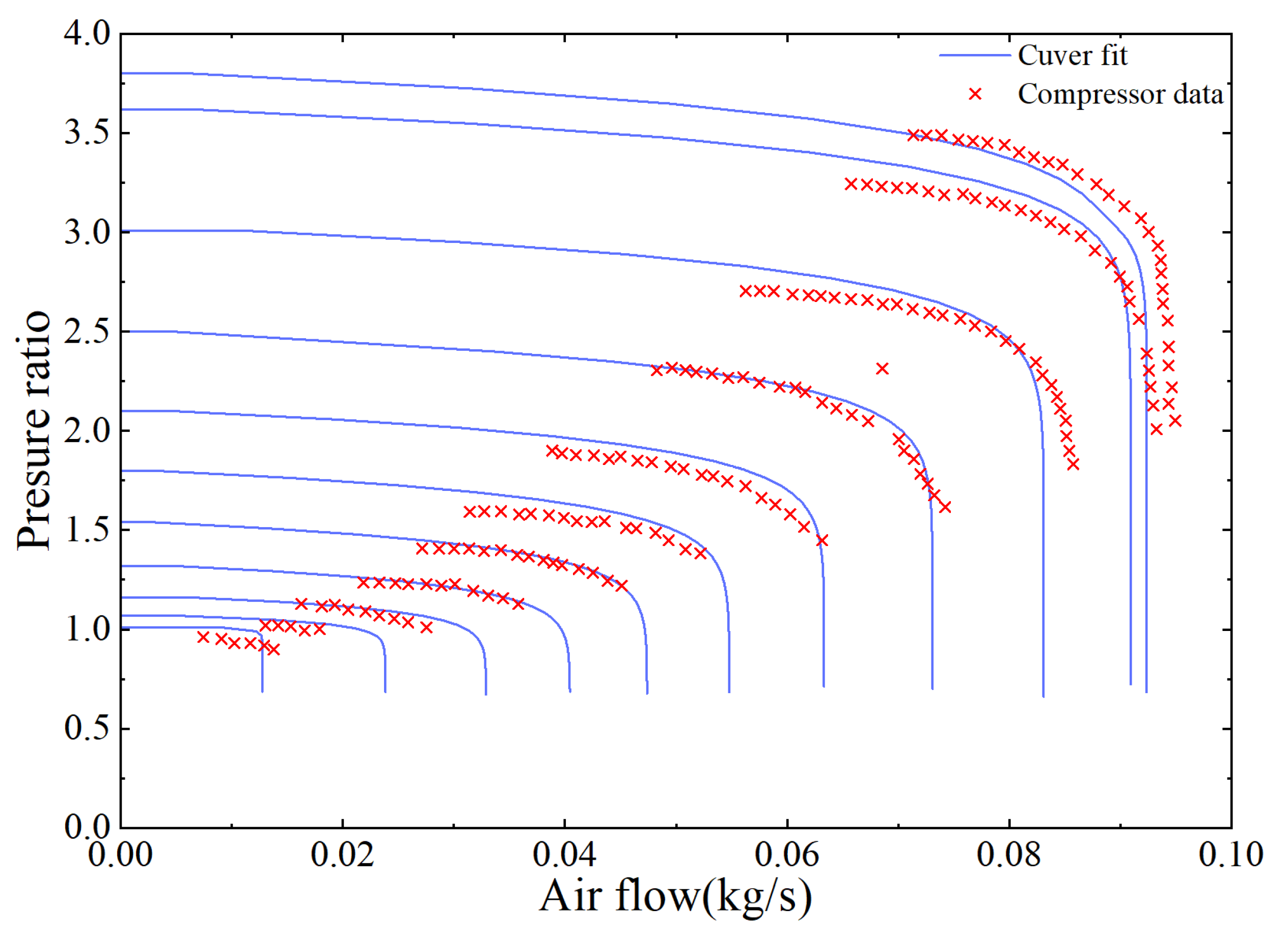
Appendix B.1. Air Compressor Modeling
Appendix B.2. Manifold Modeling and Return Manifold Modeling
Appendix B.3. Air Cooler Modeling
Appendix B.4. Air Humidifier Modeling
Appendix B.5. Hydrogen Supply System

| Symbol | Variable | Value |
|---|---|---|
| Ratio of special heat of air | 1.4 | |
| Constant pressure-specific heat of air | ||
| Air gas constant | K) | |
| Air density | ||
| Compressor diameter | ||
| Constant | ||
| Constant | ||
| Constant | ||
| Constant | ||
| Constant | ||
| Constant | ||
| Constant | ||
| Constant | ||
| Constant | ||
| Constant | ||
| Constant | ||
| Constant | ||
| Constant | ||
| Constant | ||
| Efficiency of motor | ||
| Maximum efficiency of compressor | ||
| Combined inertia | ||
| Motor constant | ||
| Motor constant | ||
| Motor constant | ||
| Supply manifold volume | ||
| Out orifice constant | ||
| Return manifold volume | ||
| Gain | ||
| Drop | ||
| Constant term | ||
| Return manifold throttle area |
Appendix C. DDPG Algorithm Pseudocode and Hyperparameters
| Algorithm A1. Dual DDPG PID algorithm |
| 4: For episode = 1 to M do |
| 5: Initialize a random process N for action exploration |
| 7: Initialize the state of the PID controller. |
| 8: integral = 0; Prev error = 0 |
| 9: For t = 1, T do |
| from PEMFCS |
21: end for 22: end for |
| Symbol | Variable | Value |
|---|---|---|
| Actor network learning rate | ||
| Critic network learning rate | ||
| Minibatch size | 32 | |
| Discount factor | 0.99 | |
| Experience buffer length size | ||
| Noise variance | 0.3 | |
| Soft target update rate |
References
- Xia, W.; Apergis, N.; Bashir, M.F.; Ghosh, S.; Doğan, B.; Shahzad, U. Investigating the role of globalization, and energy consumption for environmental externalities: Empirical evidence from developed and developing economies. Renew. Energy 2022, 183, 219–228. [Google Scholar]
- Wang, J.; Hussain, S.; Sun, X.; Chen, X.; Ma, Z.; Zhang, Q.; Yu, X.; Zhang, P.; Ren, X.; Saqib, M.; et al. Nitrogen application at a lower rate reduce net field global warming potential and greenhouse gas intensity in winter wheat grown in semi-arid region of the Loess Plateau. Field Crops Res. 2022, 280, 108475. [Google Scholar]
- Mao, X.; Liu, S.; Tan, J.; Hu, H.; Lu, C.; Xuan, D. Multi-objective optimization of gradient porosity of gas diffusion layer and operation parameters in PEMFC based on recombination optimization compromise strategy. Int. J. Hydrogen Energy 2023, 48, 13294–13307. [Google Scholar]
- Liu, S.; Tan, J.; Hu, H.; Lu, C.; Xuan, D. Multi-objective optimization of proton exchange membrane fuel cell geometry and operating parameters based on three new performance evaluation indexes. Energy Convers. Manag. 2023, 277, 116642. [Google Scholar]
- Huang, Y.; Kang, Z.; Mao, X.; Hu, H.; Tan, J.; Xuan, D. Deep reinforcement learning based energy management strategy considering running costs and energy source aging for fuel cell hybrid electric vehicle. Energy 2023, 283, 129177. [Google Scholar]
- Mao, X.; Liu, S.; Huang, Y.; Kang, Z.; Xuan, D. Multi-flow channel proton exchange membrane fuel cell mass transfer and performance analysis. Int. J. Heat Mass Transf. 2023, 215, 124497. [Google Scholar]
- Jian, Q.; Huang, B.; Luo, L.; Zhao, J.; Cao, S.; Huang, Z. Experimental investigation of the thermal response of open-cathode proton exchange membrane fuel cell stack. Int. J. Hydrogen Energy 2018, 43, 13489–13500. [Google Scholar]
- Han, J.; Park, J.; Yu, S. Control strategy of cooling system for the optimization of parasitic power of automotive fuel cell system. Int. J. Hydrogen Energy 2015, 40, 13549–13557. [Google Scholar] [CrossRef]
- Yu, X.; Zhou, B.; Sobiesiak, A. Water and thermal management for Ballard PEM fuel cell stack. J. Power Sources 2005, 147, 184–195. [Google Scholar] [CrossRef]
- Kim, K.; von Spakovsky, M.R.; Wang, M.; Nelson, D.J. Dynamic optimization under uncertainty of the synthesis/design and operation/control of a proton exchange membrane fuel cell system. J. Power Sources 2012, 205, 252–263. [Google Scholar] [CrossRef]
- Ou, K.; Yuan, W.-W.; Choi, M.; Yang, S.; Kim, Y.-B. Performance increase for an open-cathode PEM fuel cell with humidity and temperature control. Int. J. Hydrogen Energy 2017, 42, 29852–29862. [Google Scholar] [CrossRef]
- Wang, Y.; Xu, H.; Wang, X.; Gao, Y.; Su, X.; Qin, Y.; Xing, L. Multi-sub-inlets at cathode f low-field plate for current density homogenization and enhancement of PEM fuel cells in low relative humidity. Energy Convers. Manag. 2022, 252, 115069. [Google Scholar]
- Liso, V.; Nielsen, M.P.; Kær, S.K.; Mortensen, H.H. Thermal modeling and temperature control of a PEM fuel cell system for forklift applications. Int. J. Hydrogen Energy 2014, 39, 8410–8420. [Google Scholar] [CrossRef]
- Zhao, X.; Li, Y.; Liu, Z.; Li, Q.; Chen, W. Thermal management system modeling of a water-cooled proton exchange membrane fuel cell. Int. J. Hydrogen Energy 2015, 40, 3048–3056. [Google Scholar] [CrossRef]
- Yu, S.; Jung, D. Thermal management strategy for a proton exchange membrane fuel cell system with a large active cell area. Renew. Energy 2008, 33, 2540–2548. [Google Scholar] [CrossRef]
- Liu, Z.; Chen, J.; Kumar, L.; Jin, L.; Huang, L. Model-based decoupling control for the thermal management system of proton exchange membrane fuel cells. Int. J. Hydrogen Energy 2023, 48, 19196–19206. [Google Scholar]
- Li, J.; Yang, B.; Yu, T. Distributed deep reinforcement learning-based coordination performance optimization method for proton exchange membrane fuel cell system. Sustain. Energy Technol. Assess. 2022, 50, 101814. [Google Scholar] [CrossRef]
- Yin, L.; Li, Q.; Wang, T.; Liu, L.; Chen, W. Real-time thermal Management of Open-Cathode PEMFC system based on maximum efficiency control strategy. Asian J. Control 2019, 21, 1796–1810. [Google Scholar] [CrossRef]
- Zhao, R.; Qin, D.; Chen, B.; Wang, T.; Wu, H. Thermal Management of Fuel Cells Based on Diploid Genetic Algorithm and Fuzzy PID. Appl. Sci. 2023, 13, 520. [Google Scholar] [CrossRef]
- Cheng, S.; Fang, C.; Xu, L.; Li, J.; Ouyang, M. Model-based temperature regulation of a PEM fuel cell system on a city bus. Int. J. Hydrogen Energy 2015, 40, 13566–13575. [Google Scholar] [CrossRef]
- Jia, Y.; Zhang, R.; Lv, X.; Zhang, T.; Fan, Z. Research on Temperature Control of Fuel-Cell Cooling System Based on Variable Domain Fuzzy PID. Processes 2022, 10, 534. [Google Scholar] [CrossRef]
- Yu, Y.; Chen, M.; Zaman, S.; Xing, S.; Wang, M.; Wang, H. Thermal management system for liquid-cooling PEMFC stack: From primary configuration to system control strategy. ETransportation 2022, 12, 100165. [Google Scholar]
- You, Z.; Xu, T.; Liu, Z.; Peng, Y.; Cheng, W. Study on Air-cooled Self-humidifying PEMFC Control Method Based on Segmented Predict Negative Feedback Control. Electrochim. Acta 2014, 132, 389–396. [Google Scholar] [CrossRef]
- Ou, K.; Wang, Y.-X.; Li, Z.-Z.; Shen, Y.-D.; Xuan, D.-J. Feedforward fuzzy-PID control for air flow regulation of PEM fuel cell system. Int. J. Hydrogen Energy 2015, 40, 11686–11695. [Google Scholar] [CrossRef]
- Hasheminejad, S.M.; Fallahi, R. Intelligent VIV control of 2DOF sprung cylinder in laminar shear-thinning and shear thickening cross-flow based on self-tuning fuzzy PID algorithm. Mar. Struct. 2023, 89, 103377. [Google Scholar]
- Mousakazemi, S.M.H. Control of a PWR nuclear reactor core power using scheduled PID controller with GA, based on two-point kinetics model and adaptive disturbance rejection system. Ann. Nucl. Energy 2019, 129, 487–502. [Google Scholar] [CrossRef]
- Wang, Y.-X.; Qin, F.-F.; Ou, K.; Kim, Y.-B. Temperature Control for a Polymer Electrolyte Membrane Fuel Cell by Using Fuzzy Rule. IEEE Trans. Energy Convers. 2016, 31, 667–675. [Google Scholar] [CrossRef]
- Tan, J.; Hu, H.; Liu, S.; Chen, C.; Xuan, D. Optimization of PEMFC system operating conditions based on neural network and PSO to achieve the best system performance. Int. J. Hydrogen Energy 2022, 47, 35790–35809. [Google Scholar] [CrossRef]
- Yan, C.; Chen, J.; Liu, H.; Lu, H. Model-based Fault Tolerant Control for the Thermal Management of PEMFC Systems. IEEE Trans. Ind. Electron. 2019, 67, 2875–2884. [Google Scholar] [CrossRef]
- Ahmadi, S.; Abdi, S.; Kakavand, M. Maximum power point tracking of a proton exchange membrane fuel cell system using PSO-PID controller. Int. J. Hydrogen Energy 2017, 42, 2043020443. [Google Scholar] [CrossRef]
- Li, G.; Li, Y. Temperature Control of PEMFC Stack Based on BP Neural Network. In Proceedings of the 2016 4th International Conference on Machinery, Materials and Computing Technology, Xi’an, China, 10–11 December 2016. [Google Scholar] [CrossRef]
- Song, C.; Kim, K.; Sung, D.; Kim, K.; Yang, H.; Lee, H.; Cho, G.Y.; Cha, S.W. A Review of Optimal Energy Management Strategies Using Machine Learning Techniques for Hybrid Electric Vehicles. Int. J. Automot. Technol. 2021, 22, 1437–1452. [Google Scholar]
- Zhou, Q.; Zhao, D.; Shuai, B.; Li, Y.; Williams, H.; Xu, H. Knowledge implementation and transfer with an adaptive learning network for real-time power management of the plug-in hybrid vehicle. IEEE Trans. Neural Netw. Learn. Syst. 2021, 32, 5298–5308. [Google Scholar] [PubMed]
- Inuzuka, S.; Zhang, B.; Shen, T. Real-Time HEV Energy Management Strategy Considering Road Congestion Based on Deep Reinforcement Learning. Energies 2021, 14, 5270. [Google Scholar] [CrossRef]
- Li, J.; Qian, T.; Yu, T. Data-driven coordinated control method for multiple systems in proton exchange membrane fuel cells using deep reinforcement learning. Energy Rep. 2022, 8, 290–311. [Google Scholar]
- Huang, Y.; Hu, H.; Tan, J.; Lu, C.; Xuan, D. Deep reinforcement learning based energy management strategy for range extend fuel cell hybrid electric vehicle. Energy Convers. Manag. 2023, 277, 116678. [Google Scholar] [CrossRef]
- Amphlett, J.C.; Baumert, R.M.; Mann, R.F.; Peppley, B.A.; Roberge, P.R. Performance modeling of the Ballard Mark IV solid polymer electrolyte fuel cell. J. Electrochem. Soc. 1995, 142, 9–15. [Google Scholar]
- Lee, J.; Lalk, T.; Appleby, A. Modeling electrochemical performance in large scale proton exchange membrane fuel cell stacks. J. Power Sources 1998, 70, 258–268. [Google Scholar]
- Mann, R.F.; Amphlett, J.C.; Hooper, M.A.; Jensen, H.M.; Peppley, B.A.; Roberge, P.R. Development and application of a generalised steady-state electrochemical model for a PEM fuel cell. J. Power Sources 2000, 86, 173–180. [Google Scholar]
- Nguyen, T.V.; White, R.E. A Water and Heat Management Model for Proton-Exchange-Membrane Fuel Cells. J. Electrochem. Soc. 1993, 140, 2178–2186. [Google Scholar]
- Guzzella, L. Control Oriented Modelling of Fuel-Cell Based Vehicles. In Presentation in NSF Workshop on the Integration of Modeling and Control for Automotive Systems; University of Michigan: Ann Arbor, MI, USA, 1999. [Google Scholar]
- Pukrushpan, J.T.; Peng, H.; Stefanopoulou, A.G. Control-Oriented Modeling and Analysis for Automotive Fuel Cell Systems. J. Dyn. Syst. Meas. Control 2004, 126, 14–25. [Google Scholar] [CrossRef]
- Xing, L.; Chang, H.; Zhu, R.; Wang, T.; Zou, Q.; Xiang, W.; Tu, Z. Thermal analysis and management of proton exchange membrane fuel cell stacks for automotive vehicle. Int. J. Hydrogen Energy 2021, 46, 32665–32675. [Google Scholar]
- Hu, P.; Cao, G.-Y.; Zhu, X.-J.; Hu, M. Coolant circuit modeling and temperature fuzzy control of proton exchange membrane fuel cells. Int. J. Hydrogen Energy 2010, 35, 9110–9123. [Google Scholar] [CrossRef]
- Wang, L.; Quan, Z.; Zhao, Y.; Yang, M.; Zhang, J. Experimental investigation on thermal management of proton exchange membrane fuel cell stack using micro heat pipe array. Appl. Therm. Eng. Des. 2022, 214, 118831. [Google Scholar]
- Li, W.; Cui, H.; Nemeth, T.; Jansen, J.; Ünlübayir, C.; Wei, Z.; Feng, X.; Han, X.; Ouyang, M.; Dai, H.; et al. Cloud-based health- conscious energy management of hybrid battery systems in electric vehicles with deep reinforcement learning. Appl. Energy 2021, 193, 116977. [Google Scholar]
- Liu, Y.; Gao Po Zheng, C.; Tian, L.; Tian, Y. A deep reinforcement learning strategy combining expert experience guidance for a fruit-picking manipulator. Electronics 2022, 11, 311. [Google Scholar] [CrossRef]
- Hu, H.; Lu, C.; Tan, J.; Liu, S.; Xuan, D. Effective energy management strategy based on deep reinforcement learning for fuel cell hybrid vehicle considering multiple performance of integrated energy system. Energy Res. 2022, 46, 24254–24272. [Google Scholar]
- Pukrushpan, J.T. Modeling and Control of Fuel Cell Systems and Fuel Processors; University of Michigan: Ann Arbor, MI, USA, 2003. [Google Scholar]
- Cunningham, J.M.; Hoffman, M.A.; Moore, R.M.; Friedman, D.J. Requirements for a Flexible and Realistic Air Supply Model for Incorporation into a Fuel Cell Vehicle (FCV) System Simulation; SAE International: Warrendale, PA, USA, 1999. [Google Scholar]
- Moraal, P.; Kolmanovsky, I. Turbocharger Modeling for Automotive Control Applications; SAE International: Warrendale, PA, USA, 1999. [Google Scholar] [CrossRef]
| Parameter | Description | Value |
|---|---|---|
| 0.7 | ||
| 0.8 | ||
| on the reward | 0.2 | |
| on the reward | 0.3 | |
| base reward | 3 | |
| base reward | 4 | |
| , penalties for deviations from target values | −1 | |
| , penalties for deviations from target values | −0.9 | |
| Constant offset value used to adjust the overall output of the reward function | 0.2 |
| Control Algorithm | Parameters | Parameter Range | Convergence Accuracy | Description |
|---|---|---|---|---|
| PSO-PID | KP | 0.01~0.03 | 0.001 | PSO optimizes PID controller parameters to adjust coolant flow to balance temperature changes |
| KI | 0.001~0.07 | 0.001 | ||
| KD | 0~6 | 0.001 | ||
| FUZZY-PID | KP | −0.3~0.3 | 0.001 | Fuzzy logic adjusts PID controller parameters to regulate coolant flow to equalize temperature changes |
| KI | −0.06~0.06 | 0.001 | ||
| KD | −3~3 | 0.001 |
| Control Methods | Load Time (s) | Mean Absolute Control Error (K) | Absolute Maximum Overshoot (K) | Mean Setting Time (s) |
|---|---|---|---|---|
| D-DDPG-PID | 0–200 | 0.016 | 0.31 | 33 |
| 400–600 | 0.009 | 0.26 | 29 | |
| 800–100 | 0.004 | 0.13 | 19 | |
| PID | 0–200 | 0.065 | 1.02 | 59 |
| 400–600 | 0.044 | 0.85 | 51 | |
| 800–100 | 0.021 | 0.41 | 39 | |
| FUZZY-PID | 0–200 | 0.047 | 0.79 | 53 |
| 400–600 | 0.038 | 0.74 | 47 | |
| 800–1000 | 0.020 | 0.38 | 35 | |
| PSO-PID | 0–200 | 0.033 | 0.64 | 41 |
| 400–600 | 0.0025 | 0.51 | 39 | |
| 800–100 | 0.013 | 0.25 | 22 |
Disclaimer/Publisher’s Note: The statements, opinions and data contained in all publications are solely those of the individual author(s) and contributor(s) and not of MDPI and/or the editor(s). MDPI and/or the editor(s) disclaim responsibility for any injury to people or property resulting from any ideas, methods, instructions or products referred to in the content. |
© 2025 by the authors. Licensee MDPI, Basel, Switzerland. This article is an open access article distributed under the terms and conditions of the Creative Commons Attribution (CC BY) license (https://creativecommons.org/licenses/by/4.0/).
Share and Cite
Zhang, Z.; Shen, Y.; Ou, K.; Liu, Z.; Xuan, D. PEMFC Thermal Management Control Strategy Based on Dual Deep Deterministic Policy Gradient. Hydrogen 2025, 6, 20. https://doi.org/10.3390/hydrogen6020020
Zhang Z, Shen Y, Ou K, Liu Z, Xuan D. PEMFC Thermal Management Control Strategy Based on Dual Deep Deterministic Policy Gradient. Hydrogen. 2025; 6(2):20. https://doi.org/10.3390/hydrogen6020020
Chicago/Turabian StyleZhang, Zhi, Yunde Shen, Kai Ou, Zhuwei Liu, and Dongji Xuan. 2025. "PEMFC Thermal Management Control Strategy Based on Dual Deep Deterministic Policy Gradient" Hydrogen 6, no. 2: 20. https://doi.org/10.3390/hydrogen6020020
APA StyleZhang, Z., Shen, Y., Ou, K., Liu, Z., & Xuan, D. (2025). PEMFC Thermal Management Control Strategy Based on Dual Deep Deterministic Policy Gradient. Hydrogen, 6(2), 20. https://doi.org/10.3390/hydrogen6020020