Abstract
Point events can be distributed regularly, randomly, or in clusters. A cluster of points is defined by the distance from which any point included in a cluster is farther from any other point outside the cluster. Many solutions and methods are possible to define clustering distance. I present here a simple method, nearest neighbour index clustering (NNIC), which separately identifies local clusters of points using only their neighbourhood relationships based on the nearest neighbour index (NNI). It computes a Delaunay triangulation among all points and calculates the length of each line, selecting the lines shorter than the expected nearest neighbour distance. The points intersecting the selected Delaunay lines are considered to belong to an independent cluster. I verified the performance of the NNIC method with a virtual and a real example. In the virtual example, I joined two sets of random point processes following a Poisson distribution and a Thomas cluster process. In the real example, I used a point process from the distribution of individuals of two species of Iberian lizards in a mountainous area. For both examples, I compared the results with those of the nearest neighbour cleaning (NNC) method. NNIC selected a different number of clustered points and clusters in each random set of point processes and included fewer points in clusters than the NNC method.
1. Introduction
How are events distributed across space? This is a very frequent question asked by researchers from many different disciplines, such as epidemiology [1], neurosciences [2], criminology [3], econometrics [4], agronomy [5], forestry [6], or ecology [7,8]. In these research fields, it is important to know whether events are distributed regularly, randomly, or in clusters [9]. One famous example of the importance of analysing the distribution patterns of events is the epidemiological study performed by John Snow in 1854 [10]. He related the spatial location of water pumps with the incidence of cholera in London. Thanks to his conclusions, the water pump of Broad Street was closed, and cholera abated in London. From that pioneering study, spatial analyses have improved considerably thanks to spatial statistics [11]. In a random pattern, the probability of finding an event is equal everywhere and independent of the presence of other events. In a regular pattern, the probabilities of finding events and empty areas are similar. In a clustered pattern, the probability of finding a second event near the first one and of finding areas without events are very high but mutually exclusive.
In the particular case of ecology, the analysis of the spatial distribution of events provides insights into how organisms interact with each other or with their environment [12]. However, identifying and defining clusters is not a simple task [13]. Clusters of events can be defined as a set of entities that are alike (and not like entities from different clusters), or as a region with a relatively high density of points, separated from other regions by regions with a relatively low density of points [14]. However, I will consider here a cluster of events as an aggregation of points such as the distance between any two points in the cluster is less than the distance between any point not in the cluster [14]. Therefore, the definition of what is a cluster inside a process of points depends exclusively on a threshold distance, i.e., the distance where any point included in a cluster is farther from any other point outside the cluster [13]. Points are considered clustered if the distance between them is lower than the clustering distance. Effectively, many solutions are possible to define that clustering distance, depending mainly on how points are distributed inside the study area and the size of the study area [13,14].
Spatial statistics offer us several methods for determining whether a point process has a clustered, regular, or random distribution [13]. Distance functions like Ripley’s K, G-function, F-function, or g-function, graphically represent the frequency of points at different distances against a theoretical distribution of distances [13]. Clustered distributions can also be defined by measuring the spatial autocorrelation of a variable [15] based on global statistics [16] such as Global Moran’s I [17,18] and Getis-Ord’s G statistic [19]. However, all these methods do not individually identify the points belonging to a cluster: they only indicate the type of the distribution (clustered, regular, random). Methods for local spatial autocorrelation, such as local indicators of spatial association (LISA) [20], provide means of determining clusters and outliers of autocorrelated points. Local Getis-Ord’s Gi and Gi*statistics [19] determine only hot and cold spots. Nonetheless, the researcher may not always want to measure the spatial autocorrelation of a variable but simply to identify clusters of points based on their neighbourhood relationships.
Many algorithms have been described to identify clusters and their points based exclusively on their topographical relationships, such as nearest neighbour cleaning (NNC) [21], AMOEBA [22,23], the adaptive spatial clustering algorithm based on Delaunay triangulation (ASCDT) [24], TRICLUST [25], SPATCLUS [26], the variable clumping method (VMC) [27], or CLARANS [28]. NNC [21] depends on the number of nearest neighbours to be considered. VMC uses the intersection of buffers of different sizes to identify the clustering points [27]. SPATCLUS is based on a data transformation by defining a trajectory to attribute to each point to a selection order and the distance to its nearest neighbour [26]. CLARANS determines the centre point of the clusters [28]. Other algorithms use the Delaunay triangulation to calculate distances between points (AMOEBA, ASCDT, TRICLUST). Then, different approaches are used to apply a threshold to the triangulation distances. AMOEBA uses the local Gi* [29]. ASCDT combines metrics at global and local levels [24]. TRICLUST uses the mean of the length, the standard deviation of the length divided by the mean, and the positive part of the derivative of the mean [25].
The application of most of these algorithms is complicated [24]. A simple method is necessary to quickly identify clusters of points. Here, I present a new method, nearest neighbour index clustering (NNIC) based on the nearest neighbour index (NNI) [30], which provides a quantifiable measure of the point process distribution. The method consists of computing a Delaunay triangulation and selecting the points with a distance lower than the expected nearest neighbour distance defined by the NNI.
2. Materials and Methods
NNIC is based on the nearest neighbour index (NNI) by Clark and Evans [30]. This index provides the ratio between the observed mean nearest neighbour distance of the point process and the expected distance for a Poisson point process with the same intensity (i.e., density of points). The NNI considers that a point process is clustered when the mean nearest neighbour distance is lower than the expected one. A value higher than 1 suggests order, while a value lower than 1 means clustering. A value of 0 indicates randomness. Therefore, the topographical clustering method firstly computes a Delaunay triangulation among all points and calculates the length of each line. Secondly, it computes the expected nearest neighbour distance using the formula by Clark and Evans [30]:
where A is the size of the study area, B is the perimeter, and N is the number of points. The next step is to select those Delaunay lines shorter than the expected nearest neighbour distance. The points intersecting the selected Delaunay lines are considered clustered. Those points intersecting a separated group of Delaunay triangles are considered to belong to an independent cluster (Figure 1).
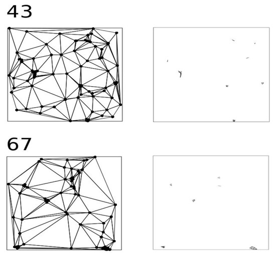
Figure 1.
Different steps of the nearest neighbour index clustering (NNIC) process. The left column of the maps correspond to the Delaunay polygons of two point processes (number 43 and 67; see Table S1); and the right column represent the selected triangles.
To verify the performance of NNIC, I merged two sets of random point processes following a Poisson distribution and a Thomas cluster process. Both datasets were joined to give clustered points inside the point process. The global distribution pattern was measured by the nearest neighbour index [30]. I implemented NNIC in R 4.0.4 software [31], with the following consecutive steps (see the script in Supplementary Material Text S1): (1) creation of a virtual study area with a size of 10 × 10 units; (2) calculation of the study area size and perimeter (A and B variables in (1)); (3) generation of random point processes including a Poisson distribution and a Thomas cluster process; (4) counting the number of points inside the window (N variable in Equation (1)); (5) calculation of the Delaunay tessellation for the point process and the length of each triangle edge; (6) calculation of the expected nearest neighbour distance using the formula in Equation (1); (7) selection of those edges with length lower than the expected nearest neighbour one; and (8) identification of clustered points by intersecting the Delaunay triangle lines and the points.
I also verified the performance of NNIC with a real example (see the script in Supplementary Material Text S2): a point process with the distribution of individuals of two species of Iberian lizards (P. carbonelli Pérez-Mellado, 1981 and P. guadarramae (Boscá, 1916)) in a mountainous area of the Iberian Peninsula (Estrela, Portugal) [32]. Estrela area is composed of rock boulders on the shore of a reservoir. Lizards were captured on 16 and 17 May 2012, and re-sighted between 19 and 24 May 2012 [32] For visual identification of wall lizards during re-sighting sampling, each lizard was marked with non-toxic coloured inks using a unique code made of three coloured dots on its back (see [32] more details). The point data is provided as Supplementary Data.
Finally, I compared NNIC in the virtual and real examples with nearest neighbour cleaning (NNC) [21], a technique for recognising features in a spatial point pattern in the presence of random clutter. For each point in the pattern, the distance to the kth nearest neighbour was computed. Then, an algorithm was used to fit a mixture distribution to the nearest neighbour distances. The mixture components represented the feature and the clutter (named as ‘noise’). The mixture model can be used to classify each point as belonging to one or another component.
3. Results
In the virtual example, NNIC selected a different number of clustered points and clusters in each random set of point processes (Table S1). Figure 2 shows several examples of NNIC results. When comparing with the NNC method, NNIC included less points in clusters (t-test: t = −5.3269, df = 190.61, p < 0.0001; Table 1 and Table S1; Figure 3). In the real example, NNIC also selected fewer points than NNC (Table 2; Figure 4). In the virtual example, NNIC identified between 8 and 66 clusters (Table 1), while in the real example NNIC identified 117 clusters (Table 2).
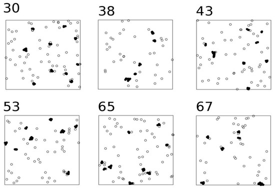
Figure 2.
Examples of NNIC using random points. Open circles are non-clustered points; black circles are clustered points. Figure numbers indicate the number of the iteration (see Table S1).

Table 1.
Summary results for the virtual example. Mean, standard deviation, minimum, and maximum number of random points, number of clustered points identified by NNIC, number of clusters identified by NNIC, and number of clustered points identified by NNC. NNIC: nearest neighbour index clustering. NNC: nearest neighbour cleaning.
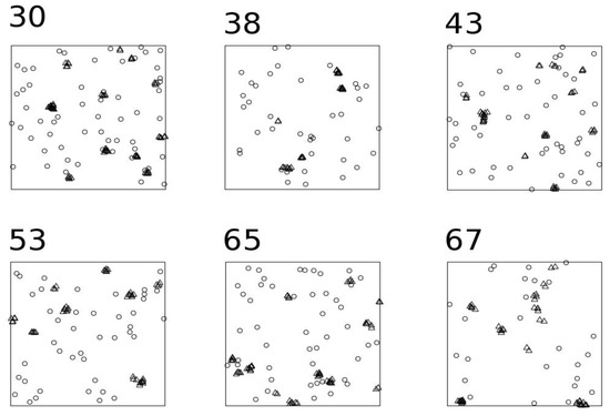
Table 2.
Summary results for the real example. N points: number of points inside the study area; NNIC points: number of clustered points identified by NNIC; NNIC clusters: number of clusters identified by NNC; NNC points: number of clustered points identified by NNC; EX NND: expected nearest neighbour distance; Z statistic from the NNI and the corresponding p-value. NNIC: nearest neighbour index clustering. NNC: nearest neighbour cleaning. NNI: nearest neighbour index.
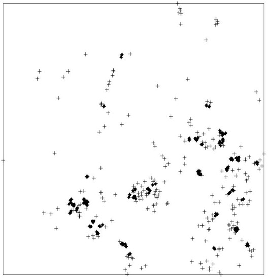
Figure 4.
Example of NNIC (Nearest Neighbour Index Clustering) using a point process with the distribution of individuals of two species of Iberian lizards in a mountainous area of the Iberian Peninsula (Estrela, Portugal). Crosses are non-clustered points; black circles are clustered points. See main text for details.
4. Discussion
The nearest neighbour index clustering method (NNIC) identified fewer clustered points than nearest neighbour cleaning (NNC) [21], for both the virtual example and the real one. The main difference between both methods is that NNIC is not only able to identify points as clustered but to assign the points to a particular cluster and to count directly the number of clusters in the study area. As represented in Figure 3, the NNC method classified the points in noise and features, but it cannot determine which features are inside the same significant group of points. NNIC uses Delaunay triangulation, like AMOEBA [22,23,29], ASCDT [24], and TRICLUST [25]. However, instead of using complex spatial criteria to define the threshold distance (ASCDT), autocorrelation (AMOEBA), or central and dispersal metrics of edge lengths (TRICLUST), it uses the expected distance from the NNI [30], an objective metric available in most GIS programs. On the other hand, the simplicity of NNIC has a cost: VMC and AMOEBA can hierarchically define sub-clusters [23,27]. NNIC can also define sub-clusters, but only by sequential analyses, i.e., searching for clusters inside a previously defined cluster. TRICLUST can effectively handle datasets with clusters of complex shapes, non-uniform densities, and a large number of noises [25]. Further research is needed to determine how NNIC deals with noise data.
As stated before, identifying and defining clusters in a point process is not a completely objective calculation: many possible solutions can be obtained, as events can be grouped in a cluster with different purposes [14]. People recognise a cluster when they see it in the planar space, but it is nearly impossible to provide a full description of objective criteria to define those clusters. This is why there are so many clustering algorithms that provide different solutions, all of them valid (e.g., Liu et al. [25]). Consequently, comparisons of clustering algorithms are mainly based on the advantages of using a particular method or how well the algorithm distinguishes the noise from relevant points [21,25]. In this sense, the main advantage of NNIC is the possibility of implementing the method in any GIS software or in R language, in a fast and simple way. Algorithms such as CLARANS, ASCDT, or TRICLUST cannot be calculated directly in a GIS software. For example, ASCDT applies a two-level strategy: a global edge cut-off statistical criterion to remove excessively long edges at a global level; and two criteria to remove inconsistent edges at a local level [24]. These functions are difficult to implement in a GIS without recurring to a programming language (e.g., Python or R). Therefore, NNIC can be applied to any situation where a simple algorithm is needed, requiring only a minimum knowledge of spatial analyses without the necessity of complex statistical computations. This is quite common in ecology. For instance, the main output of studies on animal collisions by vehicles is the definition of road-kills as independent clusters [33,34,35,36]. Other ecological studies have applied clustering methods to analyse the local spatial distribution of plants [37,38,39] and animals [9,40,41,42,43,44]. Local autocorrelation methods have been used to analyse the spatial patterns of species richness [8,45].
5. Conclusions
In summary, spatial analyses of point processes in ecological studies are focused on the identification of clusters based only on the distances among points, and uncomplicated methods are preferred. NNIC is a simple, intuitive, and fast method, requiring minimum skills from geomatics that can be calculated in any GIS program.
Supplementary Materials
The following are available online at https://www.mdpi.com/article/10.3390/ecologies2030017/s1, Table S1: Application of Nearest Neighbour Index Clustering (NNIC) and Nearest Neighbour Cleaning (NNC) methods to 100 hundred random point processes; Text S1: R script for the application of the NNIC (Nearest Neighbour Index Clustering) method using virtual data; Text S2: R script for the application of the Nearest Neighbour Index Clustering (NNIC) method using real data.
Funding
NS is partially supported by a CEEC2017 contract (CEECIND/02213/2017) from Fundação para a Ciência e a Tecnologia (FCT).
Data Availability Statement
The point data are provided as Supplementary Data.
Conflicts of Interest
The author declares no conflict of interest.
References
- Themudo, G.E.C.; Østergaard, J.; Ersbøll, A.K. Persistent spatial clusters of plasmacytosis among Danish mink farms. Prev. Veter. Med. 2011, 102, 75–82. [Google Scholar] [CrossRef]
- Prodanov, D.; Nagelkerke, N.; Marani, E. Spatial clustering analysis in neuroanatomy: Applications of different approaches to motor nerve fiber distribution. J. Neurosci. Methods 2007, 160, 93–108. [Google Scholar] [CrossRef]
- Getis, A.; Drummy, P.; Gartin, J.; Gorr, W.; Harries, K.; Rogerson, P.; Stoe, D.; Wright, R. Geographic Information Science and Crime Analysis. URISA J. 2000, 12, 7–14. [Google Scholar]
- Anselin, L.; Hudak, S.; Anselin, L.; Hudak, S. Spatial econometrics in practice: A review of software options. Reg. Sci. Urban Econ. 1992, 22, 509–536. [Google Scholar] [CrossRef]
- Fraga, H.; Santos, J.A.; Malheiro, A.; Oliveira, A.A.; Moutinho-Pereira, J.; Jones, G.V. Climatic suitability of Portuguese grapevine varieties and climate change adaptation. Int. J. Clim. 2015, 36, 1–12. [Google Scholar] [CrossRef]
- King, D.A.; Bachelet, D.M.; Symstad, A.J.; King, D.A.; Bachelet, D.M.; Symstad, A.J. Climate change and fire effects on a prairie–woodland ecotone: Projecting species range shifts with a dynamic global vegetation model. Ecol. Evol. 2013, 3, 5076–5097. [Google Scholar] [CrossRef]
- Qiao, H.; Lin, C.; Jiang, Z.; Ji, L. Marble Algorithm: A solution to estimating ecological niches from presence-only records. Sci. Rep. 2015, 5, 14232. [Google Scholar] [CrossRef]
- Nelson, T.; Boots, B. Detecting spatial hot spots in landscape ecology. Ecography 2008, 31, 556–566. [Google Scholar] [CrossRef]
- Frost, C.L.; Bergmann, P.J. Spatial Distribution and Habitat Utilization of the Zebra-tailed Lizard (Callisaurus draconoides). South Am. J. Herpetol. 2012, 46, 203–208. [Google Scholar] [CrossRef]
- Brody, H.; Rip, M.R.; Vinten-Johansen, P.; Paneth, N.; Rachman, S. Map-making and myth-making in Broad Street: The London cholera epidemic, 1854. Lancet 2000, 356, 64–68. [Google Scholar] [CrossRef]
- Anselin, L.; Rey, S.J. Perspectives on Spatial Data Analysis; Springer: Berlin/Heidelberg, Germany, 2010. [Google Scholar]
- Pianka, E.R. The Structure of Lizard Communities. Annu. Rev. Ecol. Syst. 1973, 4, 53–74. [Google Scholar] [CrossRef] [Green Version]
- Baddeley, A.; Rubak, E.; Turner, R. Spatial Point Patterns: Methodology and Applications with R.; Chapman and Hall/CRC: Boca Raton, FL, USA, 2015. [Google Scholar]
- Jain, A.K.; Dubes, R.C. Algorithms for Clustering Data; Prentice-Hall: Hoboken, NJ, USA, 1988. [Google Scholar]
- Sokal, R.R.; Oden, N.L.; Thomson, B.A. Local spatial autocorrelation in biological variables. Biol. J. Linn. Soc. 1998, 65, 41–62. [Google Scholar] [CrossRef]
- Getis, A. A History of the Concept of Spatial Autocorrelation: A Geographer ’s Perspective. Geogr. Anal. 2008, 40, 297–309. [Google Scholar] [CrossRef]
- Cliff, A.; Ord, J. Spatial Processes: Models and Applications; Pion: London, UK, 1981. [Google Scholar]
- Moran, P.A.P. Notes on Continuous Stochastic Phenomena. Biometrika 1950, 37, 17–23. [Google Scholar] [CrossRef]
- Getis, A.; Ord, J.K. The Analysis of Spatial Association by Use of Distance Statistics; Springer: Berlin/Heidelberg, Germany, 2008; pp. 127–145. [Google Scholar] [CrossRef]
- Anselin, L. Local Indicators of Spatial Association-LISA. Geogr. Anal. 2010, 27, 93–115. [Google Scholar] [CrossRef]
- Byers, S.; Raftery, A.E. Nearest-Neighbor Clutter Removal for Estimating Features in Spatial Point Processes. J. Am. Stat. Assoc. 1998, 93, 577–584. [Google Scholar] [CrossRef]
- Duque, J.C.; Aldstadt, J.; Velasquez, E.; Franco, J.L.; Betancourt, A. A computationally efficient method for delineating irregularly shaped spatial clusters. J. Geogr. Syst. 2010, 13, 355–372. [Google Scholar] [CrossRef]
- Estivill-Castro, V.; Lee, I. AMOEBA: Hierarchical Clustering Based on Spatial Proximity Using Delaunay Diagram. In Proceedings of the 9th International Symposium on Spatial Data Handling, Beijing, China, 10–12 August 2000; pp. 1–16. [Google Scholar]
- Deng, M.; Liu, Q.; Cheng, T.; Shi, Y. An adaptive spatial clustering algorithm based on delaunay triangulation. Comput. Environ. Urban Syst. 2011, 35, 320–332. [Google Scholar] [CrossRef]
- Liu, D.; Nosovskiy, G.V.; Sourina, O.; Liu, D.; Nosovskiy, G.V.; Sourina, O. Effective clustering and boundary detection algorithm based on Delaunay triangulation. Pattern Recognit. Lett. 2008, 29, 1261–1273. [Google Scholar] [CrossRef]
- Demattei, C.; Molinari, N.; Daurès, J.-P. SPATCLUS: An R package for arbitrarily shaped multiple spatial cluster detection for case event data. Comput. Methods Programs Biomed. 2006, 84, 42–49. [Google Scholar] [CrossRef] [PubMed] [Green Version]
- Okabe, A.; Funamoto, S. An Exploratory Method for Detecting Multi-Level Clumps in the Distribution of Points—A Computational Tool, VCM (Variable Clumping Method). J. Geograph. Syst. 2000, 2, 111–120. [Google Scholar] [CrossRef]
- Ng, R.T.; Han, J. Efficient and Effective Clustering Data Mining Methods for Spatial. In Proceedings of the 20th VLDB Conference, Santiago, Chile, 12–15 September 1994; pp. 144–155. [Google Scholar]
- Aldstadt, J.; Getis, A. Using AMOEBA to Create a Spatial Weights Matrix and Identify Spatial Clusters. Geogr. Anal. 2006, 38, 327–343. [Google Scholar] [CrossRef]
- Clark, P.J.; Evans, F.C. Distance to Nearest Neighbor as a Measure of Spatial Relationships in Populations. Ecology 1954, 35, 445–453. [Google Scholar] [CrossRef]
- RCoreTeam. R: A Language and Environment for Statistical Computing; R Foundation for Statistical Computing: Vienna, Austria, 2021. [Google Scholar]
- Sillero, N.; Argaña, E.; Matos, C.; Franch, M.; Kaliontzopoulou, A.; Carretero, M.A. Local Segregation of Realised Niches in Lizards. ISPRS Int. J. Geo-Inf. 2020, 9, 764. [Google Scholar] [CrossRef]
- Malo, J.E.; Suáez, F.; Díez, A. Can We Mitigate Animal-Vehicle Accidents Using Predictive Models? J. Appl. Ecol. 2004, 4, 701–710. [Google Scholar] [CrossRef]
- Sillero, N. Amphibian mortality levels on Spanish country roads: Descriptive and spatial analysis. Amphibia-Reptilia 2008, 29, 337–347. [Google Scholar] [CrossRef]
- Matos, C.; Sillero, N.; Argaña, E. Spatial analysis of amphibian road mortality levels in northern Portugal country roads. Amphibia-Reptilia 2012, 33, 469–483. [Google Scholar] [CrossRef]
- Medinas, D.; Marques, J.T.; Costa, P.; Santos, S.; Rebelo, H.; Barbosa, A.; Mira, A. Spatiotemporal persistence of bat roadkill hotspots in response to dynamics of habitat suitability and activity patterns. J. Environ. Manag. 2021, 277, 111412. [Google Scholar] [CrossRef] [PubMed]
- Wells, M.L.; Getis, A. The spatial characteristics of stand structure in Pinus torreyana. Plant Ecol. 1999, 143, 153–170. [Google Scholar] [CrossRef]
- Gray, L.; He, F. Spatial point-pattern analysis for detecting density-dependent competition in a boreal chronosequence of Alberta. For. Ecol. Manag. 2009, 259, 98–106. [Google Scholar] [CrossRef]
- Schenk, H.J.; Holzapfel, C.; Hamilton, J.G.; Mahall, B.E. Spatial ecology of a small desert shrub on adjacent geological substrates. J. Ecol. 2003, 91, 383–395. [Google Scholar] [CrossRef]
- Sillero, N.; Gonçalves-Seco, L. Spatial structure analysis of a reptile community with airborne LiDAR data. Int. J. Geogr. Inf. Sci. 2014, 28, 1709–1722. [Google Scholar] [CrossRef]
- Sillero, N.; Argaña, E.; Freitas, S.; García-Muñoz, E.; Arakelyan, M.; Corti, C.; Carretero, M.A. Short Term Spatial Structure of a Lizard (Darevskia Sp.) Community in Armenia. Acta Herpetol. 2018, 13, 155–163. [Google Scholar] [CrossRef]
- Sillero, N.; Gomes, V. Living in clusters: The local spatial segregation of a lizard community. Basic Appl. Herpetol. 2016. [Google Scholar] [CrossRef] [Green Version]
- Underwood, A.J.; Chapman, M.G. Scales of spatial patterns of distribution of intertidal invertebrates. Oecologia 1996, 107, 212–224. [Google Scholar] [CrossRef] [PubMed]
- Moody, A.L.; Thompson, W.A.; De Bruijn, B.; Houston, A.I.; Goss-Custard, J.D. The Analysis of the Spacing of Animals, with an Example Based on Oystercatchers during the Tidal Cycle. J. Anim. Ecol. 1997, 66, 615. [Google Scholar] [CrossRef]
- Manrique, O.L.H.; Sánchez-Fernández, D.; Verdú, J.R.; Numa, C.; Galante, E.; Lobo, J.M. Using local autocorrelation analysis to identify conservation areas: An example considering threatened invertebrate species in Spain. Biodivers. Conserv. 2012, 21, 2127–2137. [Google Scholar] [CrossRef]
Publisher’s Note: MDPI stays neutral with regard to jurisdictional claims in published maps and institutional affiliations. |
© 2021 by the author. Licensee MDPI, Basel, Switzerland. This article is an open access article distributed under the terms and conditions of the Creative Commons Attribution (CC BY) license (https://creativecommons.org/licenses/by/4.0/).