Communication

Mathematical Modeling and Stability Analysis of Agri-Food Tomato Supply Chains via Compartmental Analysis

by
Israel Benítez-García
1,
Yasser A. Davizón
2,*,
Carlos Hernandez-Santos
3,*,
Nain de la Cruz
4,
Amadeo Hernandez
5,
Aureliano Quiñonez-Ruiz
2,
Eric D. Smith
6,
Jaime Sánchez-Leal
6 and
Neale R. Smith
7
1
Unidad Académica de Ingeniería en Biotecnología, Universidad Politécnica de Sinaloa (UPSIN), Mazatlán 82199, Sinaloa, Mexico
2
Tecnológico Nacional de México/IT Los Mochis, Juan de Dios, Batiz y 20 de Noviembre, Los Mochis 81259, Sinaloa, Mexico
3
Tecnológico Nacional de México/IT de Nuevo León, México, Av. Eloy Cavazos 2001, Guadalupe 66170, Nuevo León, Mexico
4
Centro de Investigación y de Estudios Avanzados del IPN, Unidad Monterrey, Vía del Conocimiento 201, Parque de Investigación e Innovación Tecnológica, Apodaca 66600, Nuevo León, Mexico
5
Tecnológico Nacional de México/IT de Pachuca, Mexico, Blvd. Felipe Ángeles Km. 84.5, Venta Prieta, Pachuca de Soto 42083, Hidalgo, Mexico
6
Industrial, Manufacturing and Systems Engineering Department, University of Texas at El Paso (UTEP), El Paso, TX 79968, USA
7
School of Engineering and Sciences, Tecnológico de Monterrey, Monterrey 64849, Nuevo León, Mexico
*
Authors to whom correspondence should be addressed.
World 2025, 6(3), 129; https://doi.org/10.3390/world6030129
Submission received: 16 July 2025 / Revised: 17 September 2025 / Accepted: 17 September 2025 / Published: 19 September 2025

Abstract

Agri-food supply chains have experienced notable changes in recent decades, with tomatoes (Solanum lycopersicum) maintaining their status as a key global crop in terms of both production and consumption. These supply chains comprise a complex network of stakeholders—including producers, processors, distributors, and retailers—who collectively ensure the delivery of tomatoes from farms to consumers. This study develops mathematical models of agri-food tomato supply chains (AFTSCs) and examines their behavior through stability analysis and dynamic simulations based on a compartmental approach. Furthermore, the environmental impact is evaluated using a sustainability index, to which the waste diversion rate is introduced. This metric is defined as the proportion of diverted waste (i.e., materials recycled, reused, or composted) relative to the total waste generated, thereby enabling the quantification of sustainability performance within the system. Finally, a sensitivity analysis is conducted on the proposed dynamical models to validate and reinforce the findings.

1. Introduction

Agri-food supply chains (AFSCs) have undergone significant transformations in recent decades, with tomatoes (Solanum lycopersicum) remaining one of the most important crops globally in terms of production and consumption [1]. These supply chains encompass a complex network of producers, processors, distributors, and retailers working together to bring tomatoes from the field to consumers. In recent years, several factors have influenced the structure and efficiency of these AFSCs, including technological advancements, changes in agricultural policies, and an increasing focus on sustainability [2].
The period from 2019 to 2024 witnessed significant technological advancements impacting tomato supply chains [3,4]. Technologies such as precision agriculture, the Internet of Things, and blockchain have enhanced traceability, resource management, and logistical efficiency. Additionally, blockchain has been used to improve transparency and food safety, allowing consumers to trace the origins of tomatoes and verify that sustainable practices are employed in the supply chain [5].
Sustainability has become a key criterion in managing tomato supply chains, and agricultural policies in various regions have started to focus on sustainable farming practices to reduce environmental impacts [6]. Recent research suggests that integrating sustainable farming practices not only improves the AFSC efficiency but also increases the resilience to climate change and market fluctuations [7]. Mathematical modeling has emerged as a critical tool in optimizing and managing AFSCs, including those for tomatoes [8]. These models assist in understanding complex systems, predicting outcomes, and improving decision-making processes. Various types of models, such as linear programming, simulation models, and stochastic models, have been applied to different aspects of the tomato supply chain [9]; here, insufficient cold chain infrastructure represents a major obstacle in the tomato supply chain. A lack of adequate refrigerated storage facilities and transportation systems causes post-harvest losses and quality deterioration, especially in regions with high temperatures. Without adequate cold chain infrastructure, farmers struggle to maintain the freshness and shelf life of their products, impacting the overall supply chain efficiency. For example, the authors of [10] proposed to enhance the traceability and transparency of tomato supply chains, ensuring product quality and safety. These mathematical models have not only contributed to efficiency improvements but have also played a role in enhancing sustainability. By optimizing resource use and reducing waste, mathematical models support the development of more sustainable supply chains. In contrast, the author employs mathematical modeling for an uncertain agricultural supply chain network. Aspects of social, economic, and environmental sustainability are incorporated into the design of the supply chain by the model.
The remainder of this article is presented as follows: Section 2 presents a literature review on the agri-food tomato supply chain. In Section 3, the mathematical models of AFTSC systems are analyzed. Section 4 provides a stability analysis for the AFTSC systems. Section 5 presents a sensitivity analysis. In addition, Section 6 presents results with simulations for the dynamic AFTSC systems 1 and 2. Finally, in Section 7, conclusions are presented, along with future research directions.

2. Agri-Food Tomato Supply Chains: Literature Review

2.1. Agri-Food Tomato Supply Chains (AFTSCs)

New perspectives and insights into sustainable global agricultural produce supply chains are emerging [11]. The value of global agriculture has increased by 89% in real terms over the past two decades, reaching USD 3.8 trillion in 2022, while the proportion of the global workforce employed in agriculture decreased from 40% in 2000 to 26% in 2022 [12,13]. Tomatoes, known for their high nutritional value, are one of the most consumed vegetables in the world and play a crucial role in the global food system. In 2021, the U.S. produced 2.9 million metric tons of fresh tomatoes, and Mexico’s tomato production grew from 2.45 million metric tons in 2011 to 4.14 million metric tons in 2020. Most of these tomatoes were exported to the United States. In 2021, the value of tomatoes imported from Mexico was USD 2.39 billion, the highest among all vegetables imported from Mexico [14,15]. The sustainability of global agricultural produce supply chains is crucial for food security, environmental protection, and socio-economic development. Globalization and technological advancements are key forces shaping sustainability, despite challenges such as resource constraints and environmental pressures. Innovative technologies, optimized organizational models, and stakeholder engagement are essential for sustainable development, impacting society, the environment, and the economy.
The supply chain plays a crucial role in enhancing agricultural value by ensuring the efficient movement of products from farms to consumers. By transporting food products from regions with low production costs to areas with high demand, the supply chain helps to balance food supply and optimize resource use. Modern supply chains incorporate advanced technologies for better tracking, storage, and transportation, reducing waste and improving product quality, as shown in Figure 1. A well-functioning supply chain supports economic development by creating jobs, reducing costs, and increasing market access for producers [16].
The agri-food supply chain for tomatoes is a complex system influenced by various factors, including production, transportation, storage, and market demand [17]. Mathematical models designed to analyze the stability and efficiency of tomato supply chains may incorporate variables such as production rates, spoilage rates, transportation delays, and market fluctuations. The findings highlight critical points where interventions can enhance stability and reduce waste. The results obtained with mathematical models provide valuable insights for policymakers and stakeholders to optimize supply chain operations, ensuring a steady and reliable supply of tomatoes from farm to table [18]. Mathematical modeling in agri-food tomato supply chains is a significant trend that helps to describe how production changes due to environmental conditions such as demand, warehouse capacity, shipping capacity, costs, and climate change, as well as factors such as the COVID-19 pandemic [19]. For example, the authors of [20] sought to summarize the impact of COVID-19 on the food supply chain, highlighting the opportunities created by the pandemic and recommending that more robust measures be undertaken in the production, processing, and delivery of food.
The AFSC is crucial for several reasons, such as the optimization of resources, including water, fertilizers, and labor, ensuring that the production process is cost-effective and sustainable. Furthermore, mathematical models can predict crop yields, helping farmers to plan better and reduce waste [21]. In addition, a mathematical model can identify bottlenecks and inefficiencies in the supply chain, from production to distribution, ensuring a steady and reliable supply of tomatoes to the market [22]. Above all, assessing the risks related to environmental changes, market fluctuations, and other uncertainties allows stakeholders to make informed decisions and mitigate potential losses in tomato production.
In general, mathematical models for the supply chain have considered various uncertainties such as the unemployment rate, water consumption by crops, the deterioration rate, the Brix of tomatoes, and the ideal yield factor of agricultural lands. These factors are treated as fuzzy variables due to their inherent uncertainty, making the model more practical and closer to real-world conditions for decision-makers and executors. One can provide a comprehensive depiction of the U.S. fresh tomato supply chain using a mathematical model. Employing the supply chain mapping approach, this article aims to detail the various production practices, intermediary linkages, and marketing channels. By focusing on the case of fresh tomatoes from Florida, the study illustrates the supply chain dynamics and interactions among stakeholders, ultimately aiming to enhance the understanding and efficiency of the fresh tomato supply chain in the United States.

2.2. Mathematical Modeling of Agri-Food Tomato Supply Chains

The optimization of agri-food supply chains (AFSCs) is crucial for addressing global challenges such as maintaining food security, sustainability, and economic viability. Within this context, the tomato supply chain stands out for its particular complexity, driven by the crop’s high perishability, seasonality, sensitivity to quality, and often globalized distribution networks [23,24,25,26]. Mathematical modeling has emerged as a powerful tool for addressing these challenges, providing decision-making frameworks that enhance efficiency, minimize waste, and strengthen resilience to disruptions [27,28,29,30].
The body of literature on mathematical applications in AFSCs is extensive and continues to expand. Early foundational reviews offered broad overviews of modeling approaches in agricultural supply chains [31], while others addressed specific topics such as loss minimization [30] or fresh-fruit optimization [32]. Subsequent studies examined harvest and production planning [33], the use of mathematical programming in fresh agri-food chains [34], and thematic reviews on models for perishable products [35]. More recently, the role of emerging technologies has been highlighted, including digitalization for sustainability [36], big data analytics [37,38], machine learning [39], and digital twins [40].
This lack of a consolidated review hinders a clear understanding of the evolution of model types, the specific operational constraints addressed (e.g., perishability [41] and ripeness [42]), and the key objectives optimized (e.g., profit [43], sustainability [44], and resilience [45]). It also limits the ability to identify emerging trends, such as the integration of sustainability metrics [46], the assessment of ecological balances [47], and the incorporation of consumer preferences [48].
Therefore, this review on mathematical methods for tomato AFSC considers the following:
  • Systematically classifying the mathematical techniques (e.g., MILP, MINLP, stochastic programming, and simulation [49]) specifically deployed for tomato supply chain optimization;
  • Identifying and analyzing the primary objectives, including economic viability, environmental sustainability [50], social aspects, loss minimization, and resilience enhancement;
  • Examining the incorporation of critical real-world constraints such as perishability, quality decay [51], ecologically based disruption risks [52], and geographical factors [53];
  • Mapping the evolution of modeling complexity and highlighting emerging trends, including the integration of AI [54,55], IoT, and other Industry 4.0 technologies with operational research models.

3. Mathematical Modeling

3.1. The Role of Compartmental Analysis in Agri-Food Tomato Supply Chains (AFTSCs)

The proposed mathematical model for an AFTSC is based on compartmental analysis using first-order differential equations. Compartmental analysis is classified into two types: (1) for continuous systems and (2) for discrete systems. In general, this type of analysis has been used to model epidemics and dynamic systems with the analogy of modeling problems such as rumors and corruption or systems where a balance between inputs and outputs in each compartment can be validated.
Compartmental analysis in supply chains serves a role comparable to its applications in fields such as epidemiology, pharmacokinetics, and ecology. In each case, it provides a structured representation of the system through inventories and flows (production rates, dissipation rates, demand rate, and throughput), which makes the underlying dynamics more transparent and amenable to analysis. Within supply chains, its distinctive value lies in linking operational decision-making to system-wide behavior. This connection helps to explain critical phenomena, including oscillatory dynamics, and potential instabilities across the network. Additionally, flows between compartments capture core activities such as production, replenishment, consumption, and demand variations. This formalization clarifies the role of each echelon and enables analysis of how decisions and disturbances propagate across the network, shaping its stability, efficiency, and resilience.
This perspective makes the following possible: (1) applying Lyapunov stability analysis to determine whether the system settles to equilibrium; (2) studying the sensitivity of the supply chain to parameters; (3) comparison with other domains, where oscillations, persistence, or divergence appear depending on the flow dynamics. In previous research works, these approaches have been addressed [56,57].
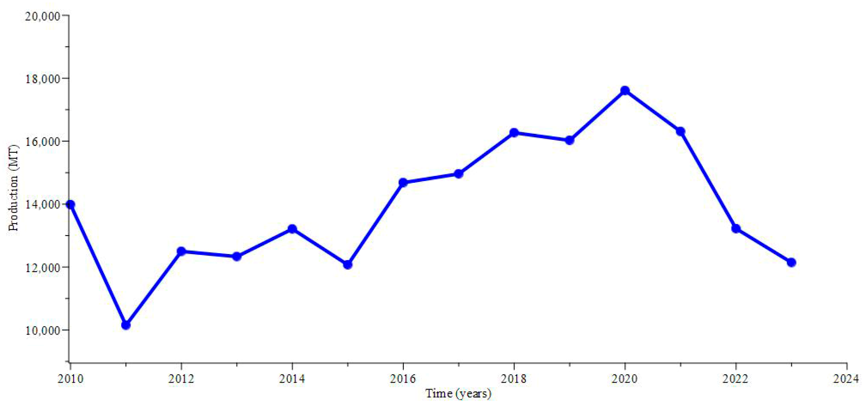
In this research, we assume that the production for the tomato supply chain approaches high volume, as shown in Figure 2 (where MT refers to metric tons). We aim to propose the use of compartmental analysis for mathematical modeling purposes, using first-order differential equations, which is suitable in terms of the agri-food tomato supply chain, considering the high volume of material in systems 1 and 2, with a proper dynamic.
Therefore, compartmental analysis in the agri-food tomato supply chain provides a formal framework to understand, predict, and improve product and information flows by capturing the critical dynamics of perishability and variability. This approach supports more informed decision-making aimed at enhancing efficiency, reducing losses, and strengthening system sustainability.
In general, the mathematical model of an AFTSC follows a first-order differential equation:
C d I d t = u φ I γ I .
In Equation (1), C is the maximum capacity of production, u refers to the demand rate for tomatoes, I refers to the inventory level, φ is the tomato production rate of the supply chain echelon, and Υ refers to the tomato decrease rate at this stage.
For two supply chain echelons with a decrease, the dynamics are as follows:
C 1 d I 1 d t = u φ 12 I 1 γ 1 I 1
and
C 2 d I 2 d t = φ 12 I 1 γ 2 I y I

3.2. Mathematical Modeling of an AFTSC with Decrease: System 1

In this section, system 1 is presented, which corresponds to a serial structure applying compartmental analysis to the mathematical model of an AFTSC with a decrease. The serial structure is based on three echelon supply chains. Figure 3 presents the dynamics for the serial structure, where systematically, the decrease in tomatoes is present at each stage of the supply chain for Producers (P), Distributors (D), and Consumers (C).
When applying compartment analysis, the set of differential equations that describe system 1 is as follows:
C 11 d I 11 d t = u 1 φ 12 I 11 γ 1 I 11
C 21 d I 21 d t = φ 12 I 11 γ 2 I 21 φ 23 I 21
and
C 31 d I 31 d t = φ 23 I 21 γ 3 I 31 y 1 I 31

3.3. Mathematical Modeling of an AFTSC with a Decrease and Reprocessing: System 2

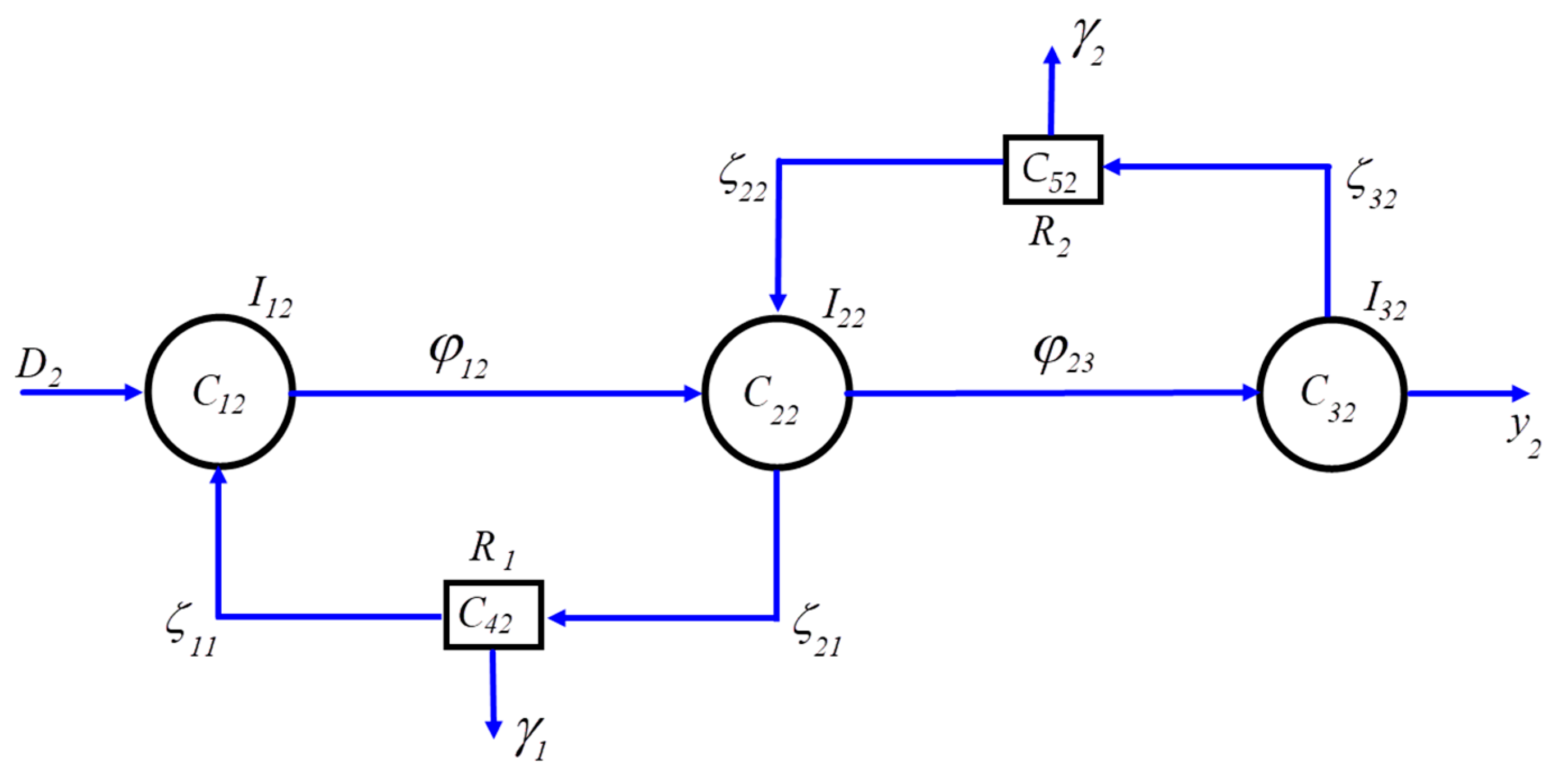
In system 2, the mathematical model for AFTSC with a decrease and reprocessing is presented. This structure adds two modules between the supply chain echelons; tomatoes can re-enter the previous stage of the supply chain, which can reprocess the previous decrease. Figure 4 establishes the mathematical model for an AFTSC with a decrease and reprocessing, which corresponds to system 2 by means of compartment analysis.
The set of differential equations, which describe the dynamics for system 2, is as follows:
C 12 d I 12 d t = u 2 + ζ 11 R 1 φ 12 I 12
C 22 d I 22 d t = φ 12 I 12 + ζ 12 R 2 φ 23 I 22 ζ 21 I 22
C 32 d I 32 d t = φ 23 I 22 ζ 32 I 32 y 2 I 32
C 42 d R 1 d t = ζ 21 I 22 ζ 11 R 1 γ 1 R 1
and
C 52 d R 2 d t = ζ 32 I 32 ζ 22 R 2 γ 2 R 2
In order to quantify the environmental impact, via a sustainability index, in Appendix B, we present the waste diversion rate, which in practical terms is the weight of the diverted waste (recycled, reused, or composted) divided by the total waste generated.
In relation to Table 1, we compare the sustainability index related to the waste diversion rate and the production metrics in steady state; the following analysis is present:
1.
Sustainability index: the waste diversion rate, which is approximated by the system 1 and system 2 ratios, expresses that, in system 2, better waste management is performed η 2 = 43.7 % with sustainability approaches, as compared with system 1 in which the sustainability index presents lower value η 1 = 26.6 % .
2.
Steady state production: from the simulation parameters in Section 6, W I P 2 = 500 in system 2, which is a lower WIP, indicating efficient and agile work, as compared to the WIP in system 1, W I P 1 = 2200 , which present tasks that are in progress and not fully accomplished.

4. Stability Analysis

Considering the mathematical models presented in Section 3 for systems 1 and 2, the stability of these systems is analyzed via Lyapunov stability analysis in this section.

4.1. Stability Analysis: System 1

Theorem 1.
The serial supply chain, for system 1, is asymptotically stable if the following holds for the candidate Lyapunov function  V · 1 I 11 , I 21 , I 31 < 0 :
φ 12 + γ 1 C 11 > 0 ,   φ 23 + γ 2 C 21 > 0 ,   γ 3 + y 1 C 31 > 0 .
Proof of Theorem 1.
The stability analysis for system 1 is given by Lyapunov stability, which is presented as follows:
We make u 1 = 0 , of which system 1 is defined by
I · 11 = k 1 I 11
I · 21 = k 2 I 11 k 3 I 21
and
I · 31 = k 4 I 21 k 5 I 31
where
k 1 = φ 12 + γ 1 C 11
k 2 = φ 12 C 21
k 3 = φ 23 + γ 2 C 21
k 4 = φ 23 C 31
and
k 5 = γ 3 + y 1 C 31
A candidate Lyapunov function of the form is proposed:
V 1 I 11 , I 21 , I 31 = 1 2 I 11 2 + 1 2 I 21 2 + 1 2 I 31 2
Deriving Equation (20), we have:
V · 1 = I 11 I · 11 + I 21 I · 21 + I 31 I · 31 .
Substituting the system of Equations (12)(14) into Equation (21), we have
V · 1 = I 11 k 1 I 11 + I 21 k 2 I 11 k 3 I 21 + I 31 k 4 I 21 k 5 I 31 .
Developing the algebra of Equation (22), we have
V · 1 = k 1 I 11 2 k 3 I 21 2 k 5 I 31 2 + k 2 I 11 I 21 + k 4 I 21 I 31 .
Applying the Lyapunov condition, for stability V · 1 < 0 , we have
V · 1 = k 1 I 11 2 k 3 I 21 2 k 5 I 31 2 .
Finally, for system 1, the Lyapunov stability yields
k 1 = φ 12 + γ 1 C 11 > 0  
k 3 = φ 23 + γ 2 C 21 > 0
and
k 5 = γ 3 + y 1 C 31 > 0

4.2. Stability Analysis: System 2

Theorem 2.
The serial supply chain with reprocessing, for system 2, is asymptotically stable if the following holds for the candidate Lyapunov function  V · 2 I 12 , I 22 , I 32 , R 1 , R 2 < 0 :
φ 12 C 12 > 0 ,   φ 12 C 22 > 0 ,   ζ 32 + y 2 C 32 > 0 ,   ζ 11 + γ 1 C 42 > 0 ,   ζ 22 + γ 2 C 52 > 0
Proof of Theorem 2.
For system 2, the Lyapunov stability analysis is as follows:
In a similar procedure, let u 2 = 0 , for which the candidate Lyapunov function is
V 2 I 12 , I 22 , I 32 , R 1 , R 2 = 1 2 I 12 2 + 1 2 I 22 2 + 1 2 I 32 2 + 1 2 R 1 2 + 1 2 R 2 2
By deriving Equation (28), we achieve the following relation:
V · 2 = I 12 I · 12 + I 22 I · 22 + I 32 I · 32 + R 1 R · 1 + R 2 R · 2
By substituting the system equation for system 2 (refer to Appendix A) into Equation (29) and simplifying, we have
V · 2 = l 2 I 12 2 l 3 I 22 2 l 7 I 32 2 l 9 R 1 2 l 11 R 2 2 + l 1 I 12 R 1 + l 3 I 22 I 12 + l 4 I 22 R 2 + l 6 I 32 I 22 +    l 8 I 22 R 1 + l 10 I 32 R 2
For Equation (30), applying the Lyapunov condition, for stability V · 1 < 0 , we have
V · 2 = l 2 I 12 2 l 3 I 22 2 l 7 I 32 2 l 9 R 1 2 l 11 R 2 2
For system 2, the Lyapunov stability is
l 2 = φ 12 C 12 > 0
l 3 = φ 12 C 22 > 0
l 7 = ζ 32 + y 2 C 32 > 0
l 9 = ζ 11 + γ 1 C 42 > 0
and
l 11 = ζ 22 + γ 2 C 52 > 0
From this stability analysis, when the Lyapunov asymptotic stability is not satisfied in an inventory system, the supply chain dynamics typically manifest as persistent or amplifying fluctuations in inventory levels. This behavior constitutes the operational manifestation of the bullwhip effect, with excessive inventory accumulation and escalating operational costs. To mitigate these instabilities, it is essential to adopt stabilization strategies such as moderating corrective responsiveness, incorporating order-smoothing mechanisms, and implementing appropriate structural constraints.

5. Sensitivity Analysis

In general, a steady-state sensitivity analysis for engineering, biological, and economic systems is ultimately evaluated at the equilibrium operating point (e.g., production rate, steady inventory, cycle time). The benefit of a steady-state sensitivity analysis in AFSCs is that it reveals how the parameters influence the long-term behavior of the system, without the need to follow its complete transient evolution. In systems 1 and 2, we might only care about the long-run average level of the inventory levels.
The general procedure is to construct the Jacobian for the system f x , θ with respect to states of the form: J x = d f d x ; therefore, it is required that J θ = d f d θ . In a steady state, assuming the system achieves an equilibrium x* such as f x * , θ = 0 , the sensitivity analysis becomes
J x x * , θ S * + J θ x * , θ = 0 ,
from which, we have
S * = J x 1 J θ ,
where Equation (38) expresses the sensitivity matrix for the steady state.

5.1. Sensitivity Analysis: System 1

For system 1, we construct the Jacobian: A x , θ = f x .
Therefore, with x 1 , x 2 , x 3 = I 11 , I 12 , I 13 ,
A x , θ = φ 12 + γ 1 C 11 0 0 φ 12 C 21 φ 23 + γ 2 C 21 0 0 φ 23 C 31 y 1 + γ 3 C 31 ,
where the parameters are θ = C 11 , C 21 , C 31 , φ 12 , φ 23 , γ 1 , γ 2 , γ 3 , y 1 .
Considering the sensitivity analysis for steady states of system 1, we have
x 1 * = u 1 φ 12 + γ 1 ,
x 2 * = u 1 φ 12 φ 12 + γ 1 φ 23 + γ 2 ,
x 3 * = u 1 φ 12 φ 23 φ 12 + γ 1 φ 23 + γ 2 y 1 + γ 3
We calculate the absolute sensitivities as follows:
ð x 1 * u 1 = 1 φ 12 + γ 1 ,
ð x 2 * ð u 1 = φ 12 φ 12 + γ 1 φ 23 + γ 2 ,
and
ð x 3 * ð u 1 = φ 12 φ 23 φ 12 + γ 1 φ 23 + γ 2 y 1 + γ 3 .
The absolute sensitivities for the inventory level at equilibrium, x 1 * , are
ð x 1 * φ 12 = u 1 φ 12 + γ 1 2 ,
and
ð x 1 * γ 1 = u 1 φ 12 + γ 1 2 .
The absolute sensitivities for the inventory level at equilibrium, x 2 * and x 3 * , are
ð x 2 * φ 12 = u 1 φ 12 + γ 1 φ 23 + γ 2 u 1 φ 12 φ 12 + γ 1 2 φ 23 + γ 2 ,
ð x 2 * γ 2 = u 1 φ 12 φ 12 + γ 1 φ 23 + γ 2 2 ,
ð x 2 * φ 23 = u 1 φ 12 φ 12 + γ 1 φ 23 + γ 2 2 ,
ð x 2 * γ 1 = u 1 φ 12 φ 12 + γ 1 2 φ 23 + γ 2 ,
and
ð x 3 * y 1 = u 1 φ 12 φ 23 φ 12 + γ 1 φ 23 + γ 2 y 1 + γ 3 2 .

5.2. Sensitivity Analysis: System 2

We calculate the sensitivity analysis in steady state for system 2 as follows.
The linear relations achieved from the steady equations are
I 22 * = u 2 ,
where for , we have
= ζ 11 ζ 21 ζ 11 + γ 1 + ζ 22 ζ 32 φ 23 ζ 22 + γ 2 ζ 32 + y 2 φ 23 + ζ 21 .
Based on this, the other steady states are proportional to I 22 * :
I 32 * = φ 23 ζ 32 + y 2 I 22 * ,
R 2 * = ζ 32 φ 23 ζ 22 + γ 2 ζ 32 + y 2 I 22 * ,
R 1 * = ζ 21 ζ 11 + γ 1 I 22 * ,
and
I 12 * = u 2 φ 12 + ζ 11 ζ 21 φ 12 ζ 11 + γ 1 I 22 * .
For system 2, we construct the Jacobian:
B x , θ 2 = φ 12 C 12 0 0 ζ 11 C 12 0 φ 12 C 22 φ 23 + ζ 21 C 22 0 0 ζ 22 C 22 0 φ 23 C 32 ζ 32 + y 2 C 32 0 0 0 ζ 21 C 42 0 ζ 11 + γ 1 C 42 0 0 0   ζ 32 C 52 0 ζ 22 + γ 2 C 52
In similar form, as for system 1, in order to calculate the sensitivity matrix, we apply Equation (38). Please refer to Appendix C for the analytical expression of the vector parameters J θ = d f d θ .

6. Results

In this section, the results of the simulations for systems 1 and 2 are analyzed in the context of the compartmental analysis.
Table 2 and Table 3 present the parameters for simulation of systems 1 and 2, respectively, from which the capacity level is given in MT, and the production rate, dissipation rate, throughput, and demand rates are in units of MT/day.

6.1. Simulations: System 1

Figure 5 illustrates the simulation outcomes for a three-echelon serial supply chain, incorporating explicit losses at each stage. The results indicate that the inventory levels vary across the echelons. Specifically, the first and second echelons maintain intermediate inventory levels, reflecting the balance between the incoming flows from upstream stages and the reductions due to losses. In contrast, the third echelon, representing the consumption stage serving the final customer, shows a marked increase in inventory. This accumulation arises because the product losses diminish downstream, resulting in higher stock levels at the final stage. These findings emphasize the influence of the echelon position on the inventory distribution and suggest that, even with losses, downstream stages may retain comparatively higher inventories, with important implications for planning, storage capacity, and spoilage risk. Overall, the analysis highlights the necessity of accounting for both losses and stage-specific dynamics when designing and managing serial supply chains for perishable goods such as tomatoes.

6.2. Simulations: System 2

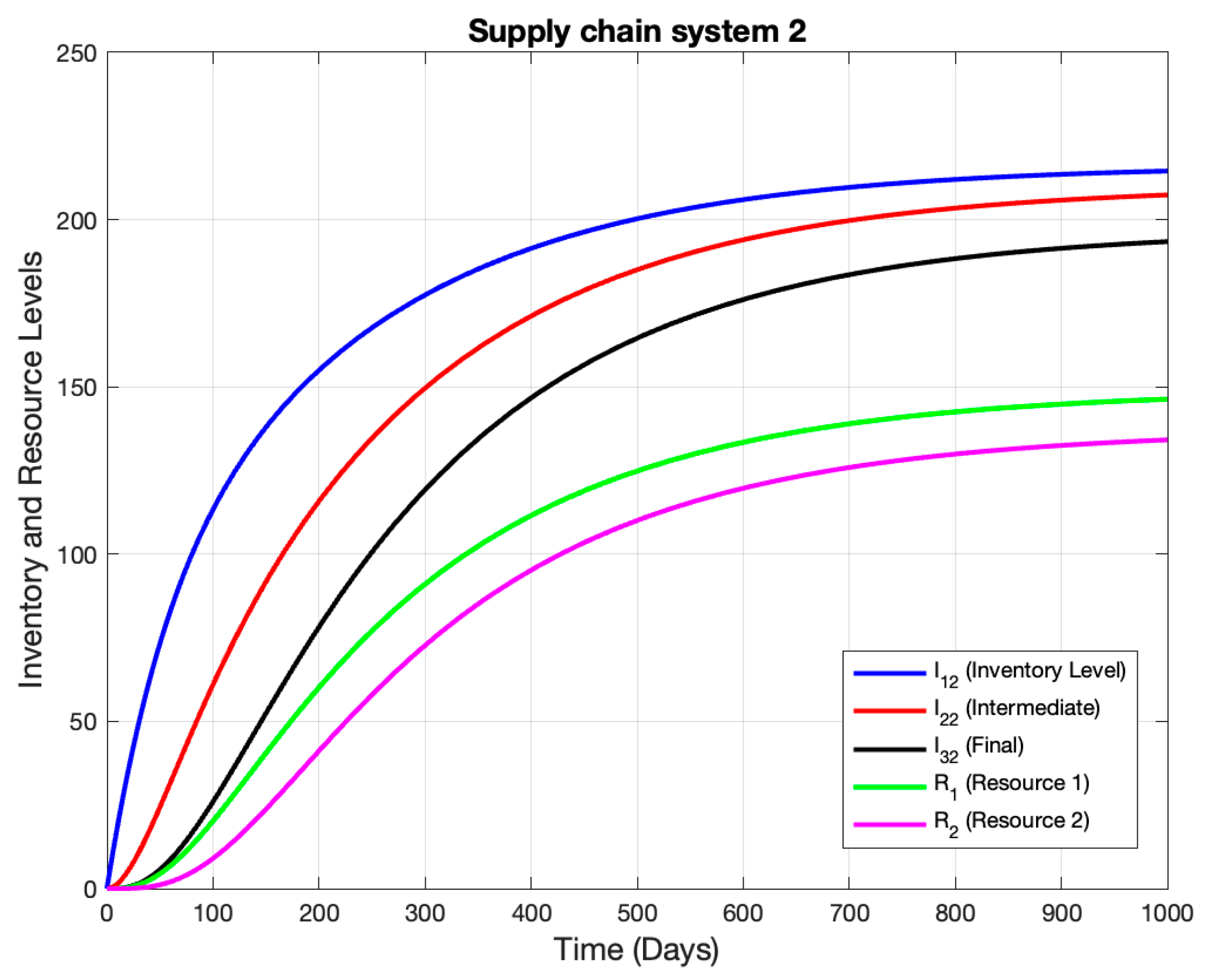
In System 2, incorporating a reprocessing mechanism, the simulation results show that the inventory levels stabilize as the recovered tomato material is reintegrated at echelons 2 and 3. This reprocessing approach not only enhances the overall inventory levels but also improves the continuity and efficiency of the raw material flows between echelons. As shown in Figure 6, the inventory levels gradually decrease from the first to the third echelon, reflecting the effect of reprocessing mitigating losses at each stage and enabling more controlled and efficient downstream material consumption. Accordingly, the reprocessing mechanism contributes to waste reduction, inventory stabilization, and a more sustainable and resource-efficient supply chain. These findings highlight the benefits of incorporating reprocessing strategies in serial supply chains for perishable products such as tomatoes, facilitating better material utilization, minimized losses, and improved alignment between the production, storage, and consumption stages.

6.3. Compartmental Analysis in Low-Variability Supply Chains

The results obtained through compartmental analysis demonstrate that low-variability supply chains tend to maintain a stable equilibrium, with smooth and well-regulated inventory levels. These findings highlight the critical importance of designing production and logistics strategies that minimize variability throughout the supply chain.

6.3.1. Variance Propagation

Compartmental analysis provides a rigorous framework to quantify how variance propagates along the supply chain. This behavior supports the use of a deterministic modeling approach, as stochastic methods—which are more appropriate for highly variable systems—offer limited additional insight in this context.

6.3.2. System Stability

The observed stability of low-variability chains shows that small disturbances in demand or production are smoothly absorbed, preventing oscillations and unnecessary accumulation of inventory levels. This confirms that a linear compartmental modeling approach is sufficient to capture the dynamic behavior of such systems, providing a reliable representation of performance under normal operating conditions.
Overall, these results not only validate the robustness of low-variability supply chains but also offer a strong mathematical foundation for justifying deterministic production and logistics strategies aimed at minimizing operational risk, maintaining efficiency, and controlling inventory costs, in future work. (Please refer to Appendix D).

7. Conclusions

This article presents a mathematical modeling framework for the tomato agri-food supply chain using a compartmental analysis approach. Two systems were formulated: the first models raw material flows with stage-wise losses, while the second adds inter-stage reprocessing to reduce these losses. Lyapunov-based stability analysis confirmed asymptotic stability for both systems, showing they can reach equilibrium under the specified operational conditions. The simulation results indicated that system 2, which incorporates the reprocessing of tomato losses, outperforms system 1 in terms of sustainability by reducing waste and improving resource utilization, highlighting the value of loss-recovery strategies and feedback mechanisms for enhancing environmental and operational efficiency in agro-food supply chains.
From a sustainability perspective, the comparative evaluation of the two systems highlighted notable differences in waste management performance. The sustainability index, measured through the waste diversion rate, indicates that system 2 achieves superior waste management, with a diversion rate of η2 = 43.7% compared to η1 = 26.6% in system 1. This result demonstrates that the incorporation of reprocessing mechanisms in system 2 significantly enhances the recovery and reuse of tomato losses along the supply chain, thereby supporting more sustainable operational practices. Regarding steady-state production metrics, the simulation results indicate that system 1 maintains a high work-in-progress (WIP) level of 2200 units, reflecting a larger number of ongoing tasks that are not yet completed. In contrast, system 2 exhibits a substantially lower WIP of 500 units, indicating a more streamlined and agile production process. The reduced WIP in system 2 not only contributes to operational efficiency but also aligns with sustainability objectives by minimizing excess inventory, reducing storage requirements, and limiting potential waste accumulation. Overall, system 2 demonstrates clear advantages over system 1 by simultaneously improving the environmental performance and production efficiency, illustrating the benefits of integrating reprocessing strategies within the tomato agri-food supply chain.
For future research, several extensions are proposed. These include the analysis of divergent and convergent supply chain structures, the integration of price dynamics, and the development of optimal control strategies that incorporate nonlinearities in the system. Such investigations would provide a more comprehensive understanding of the supply chain behavior and support the design of more resilient, efficient, and sustainable agri-food networks.

Supplementary Materials

The following supporting information can be downloaded at: https://www.mdpi.com/article/10.3390/world6030129/s1, File S1: Supply_Chain.m; File S2: Supply_Chain_2.m.

Author Contributions

Conceptualization, I.B.-G., C.H.-S., N.d.l.C., and Y.A.D.; methodology, Y.A.D. and C.H.-S.; software, N.d.l.C., A.H., and C.H.-S.; validation, A.Q.-R., N.d.l.C., Y.A.D., and N.R.S.; formal analysis, I.B.-G., Y.A.D., N.d.l.C., and C.H.-S.; investigation, Y.A.D., J.S.-L., and N.d.l.C.; resources, C.H.-S., A.Q.-R., A.H., and E.D.S.; writing—original draft preparation, I.B.-G., Y.A.D., E.D.S., and N.R.S.; writing—review and editing, C.H.-S., A.H., A.Q.-R., and J.S.-L.; supervision, C.H.-S., Y.A.D., N.d.l.C., and N.R.S.; project administration, I.B.-G., E.D.S., and C.H.-S.; funding acquisition, C.H.-S., A.H., A.Q.-R., N.d.l.C., J.S.-L., E.D.S., and N.R.S. All authors have read and agreed to the published version of the manuscript.

Funding

This research received no external funding.

Data Availability Statement

The original contributions presented in this study are included in the article and supplementary material. Further inquiries can be directed to the corresponding authors.

Conflicts of Interest

The authors declare no conflicts of interest.

Appendix A

In the Proof of Theorem 2, system 2 describes the following differential equations. Assuming u 2 = 0 :
I · 12 = l 1 R 1 l 2 I 12 ,
I · 22 = l 3 I 12 + l 4 R 2 l 5 I 22 ,
I · 32 = l 6 I 22 l 7 I 32 ,
R · 1 = l 8 I 22 l 9 R 1 ,
  R · 2 = l 10 I 32 l 11 R 2 .
Finally, for the parameters l j where j = 1 11 , we have
l 1 = ζ 11 C 12 ,   l 2 = φ 12 C 12 ,   l 3 = φ 12 C 22 ,   l 4 = ζ 12 C 22 ,   l 5 = φ 23 + ζ 21 C 22 ,   l 6 = φ 23 C 32 ,
l 7 = ζ 32 + y 2 C 32 ,   l 8 = ζ 21 C 42 ,   l 9 = ζ 11 + γ 1 C 42 ,   l 10 = ζ 32 C 52 ,   l 11 = ζ 22 + γ 2 C 52 .

Appendix B

The waste diversion rate is a key performance index (KPI) that helps to measure and improve sustainable waste management practices by measuring the success of recycling and other waste management programs. The general formula is
W a s t e   D i v e r s i o n   R a t e = W e i g h t   o f   D i v e r t e d   W a s t e T o t a l   W e i g h t   o f   W a s t e   G e n e r a t e d 100 .
In order to adapt a variant of this KPI for systems 1 and 2, we propose the following formulas:
System 1:
η 1 = γ 3 γ 1 + γ 2 + γ 3 100 ;
System 2:
η 1 = γ 2 γ 1 + γ 2 100 .

Appendix C

The explicit J θ 2 = d f d θ 2 vector for the parameters are as follows.
For demand rate u2,
f u 2 = 1 C 12 0 0 0 0 .
For the production rates:
f φ 12 = I 12 ~ C 12 I 12 ~ C 22 0 0 0 ,
f φ 23 = 0 I 22 ~ C 22 I 22 ~ C 32 0 0 .
For the dissipation rates:
f ζ 11 = R 1 ~ C 12 0 0 R 1 ~ C 42 0 ,
f ζ 21 = 0 I 22 ~ C 22 0 I 22 ~ C 42 0 ,
f ζ 22 = 0 R 2 ~ C 22 0 0 R 2 ~ C 52 ,
f ζ 32 = 0 0 I 32 ~ C 32 0 I 32 ~ C 52 ,
f γ 1 = 0 0 0 R 1 ~ C 42 0 ,
f γ 2 = 0 0 0 0 R 2 ~ C 52 .
Finally, for the throughput y2:
f y 2 = 0 0 I 32 ~ C 32 0 0

Appendix D

Table A1 presents summarized results for the performance of Systems 1 and 2, based on each system’s specific criteria, sensitivity analysis, and stability. Future work includes incorporating empirical data on dynamic systems and exploring supply networks with nonlinearities and stochastic variations in demand and variables such as price dynamics.
Table A1. Summary of performance criteria for systems 1 and 2, with respective analysis.
PerformanceSystem 1System 2
SISO linear systemsTwo dissipation stagesReprocessing and dissipation
Lyapunov stabilityAsymptotically stableAsymptotically stable
Sustainability indexLess sustainableMore sustainable
Sensitivity analysisSteady state for inventoriesSteady state for inventories
Stochastic modelingNot apply (NA)Not apply (NA)
Nonlinear systemLinear system (NA)Linear system (NA)
Empirical data validationDynamical system (NA)Dynamical systems (NA)

References

  1. Anastasiadis, F.; Apostolidou, I.; Michailidis, A. Mapping sustainable tomato supply chain in Greece: A framework for research. Foods 2020, 9, 539. [Google Scholar] [CrossRef]
  2. Granillo-Macías, R.; Rivera-Gómez, H.; González-Hernández, I.J.; Santana-Robles, F. Reconfiguration of Agrifood Supply Chain Management in Latin America during COVID-19: A Brief Literature Review. Sustainability 2024, 16, 3743. [Google Scholar] [CrossRef]
  3. Sudha, V.; Aswini, D.; Akiladevi, R. Blockchain based tomato supply chain management. In Proceedings of the 2023 2nd International Conference on Advancements in Electrical, Electronics, Communication, Computing and Automation (ICAECA), Coimbatore, India, 16–17 June 2023. [Google Scholar] [CrossRef]
  4. Akiladevi, R. A Literary Survey for Blockchain Application for Supply Chain Management of Farm Produces. In Proceedings of the 2024 Second International Conference on Emerging Trends in Information Technology and Engineering (ICETITE), Vellore, India, 22–23 February 2024. [Google Scholar] [CrossRef]
  5. Tian, F. An agri-food supply chain traceability system for China based on RFID & blockchain technology. In Proceedings of the 2016 13th International Conference on Service Systems and Service Management (ICSSSM), Kunming, China, 24–26 June 2016. [Google Scholar] [CrossRef]
  6. MacCarthy, B.L.; Ahmed, W.A.; Demirel, G. Mapping the supply chain: Why, what and how? Int. J. Prod. Econ. 2022, 250, 108688. [Google Scholar] [CrossRef]
  7. Canton, H. Food and agriculture organization of the United Nations—FAO. In The Europa Directory of International Organizations 2021; Routledge: London, UK, 2021; pp. 297–305. [Google Scholar]
  8. Albalate-Ramírez, A.; Padilla-Rivera, A.; Rueda-Avellaneda, J.F.; López-Hernández, B.N.; Cano-Gómez, J.J.; Rivas-García, P. Mapping the Sustainability of Waste-to-Energy Processes for Food Loss and Waste in Mexico—Part 1: Energy Feasibility Study. Sustainability 2024, 16, 6111. [Google Scholar] [CrossRef]
  9. Mehrbanfar, M.; Bozorgi-Amiri, A.; Nasiri, M.M. A mathematical programming model for sustainable agricultural supply chain network design under uncertainty. J. Qual. Eng. Prod. Optim. 2020, 5, 189–220. [Google Scholar] [CrossRef]
  10. Safeer, S.; Pulvento, C. Blockchain-Backed Sustainable Management of Italian Tomato Processing Industry. Agriculture 2024, 14, 1120. [Google Scholar] [CrossRef]
  11. Wang, G.; Wang, Y.; Li, S.; Yi, Y.; Li, C.; Shin, C. Sustainability in Global Agri-Food Supply Chains: Insights from a Comprehensive Literature Review and the ABCDE Framework. Foods 2024, 13, 2914. [Google Scholar] [CrossRef]
  12. Khan, M.; Papadas, D.; Arnold, L.; Behrendt, K. Sustainability challenges in the multi-tier crop agri-food sector: A systematic review. Agric. Food Econ. 2024, 12, 25. [Google Scholar] [CrossRef]
  13. FAO. World Food and Agriculture Statistical Yearbook 2024; FAO: Italy, Rome, 2024. [Google Scholar]
  14. USDA FAS. Mexico: Tomato Annual. In Livestock and Poultry: World Market and Trade; United States Department of Agriculture, Foreign Agricultural Service (USDA FAS): Washington, DC, USA, 2022. [Google Scholar]
  15. Cui, X.; Guan, Z.; Morgan, K.L.; Huang, K.-M.; Hammami, A.M. Multitiered fresh produce supply chain: The case of tomatoes. Horticulturae 2022, 8, 1204. [Google Scholar] [CrossRef]
  16. Cahyadi, E.R.; Hidayati, N.; Zahra, N.; Arif, C. Integrating Circular Economy Principles into Agri-Food Supply Chain Management: A Systematic Literature Review. Sustainability 2024, 16, 7165. [Google Scholar] [CrossRef]
  17. Nguyen, T.-D.; Nguyen-Quang, T.; Venkatadri, U.; Diallo, C.; Adams, M. Mathematical programming models for fresh fruit supply chain optimization: A review of the literature and emerging trends. AgriEngineering 2021, 3, 519–541. [Google Scholar] [CrossRef]
  18. Alemany, M.; Esteso, A.; Ortiz, Á.; del Pino, M. Centralized and distributed optimization models for the multi-farmer crop planning problem under uncertainty: Application to a fresh tomato Argentinean supply chain case study. Comput. Ind. Eng. 2021, 153, 107048. [Google Scholar] [CrossRef]
  19. Rahbari, M.; Khamseh, A.A.; Mohammadi, M. Robust optimization and strategic analysis for agri-food supply chain under pandemic crisis: Case study from an emerging economy. Expert Syst. Appl. 2023, 225, 120081. [Google Scholar] [CrossRef] [PubMed]
  20. Younis, H.; Alsharairi, M.; Younes, H.; Sundarakani, B. The impact of COVID-19 on supply chains: Systematic review and future research directions. Oper. Res. 2023, 23, 48. [Google Scholar] [CrossRef]
  21. Fang, S.-L.; Kuo, Y.-H.; Kang, L.; Chen, C.-C.; Hsieh, C.-Y.; Yao, M.-H.; Kuo, B.-J. Using sigmoid growth models to simulate greenhouse tomato growth and development. Horticulturae 2022, 8, 1021. [Google Scholar] [CrossRef]
  22. Garrido, A.; Gil-González, A.B.; García, I.; Calderón, M.; Baños, R. Using LEL and Scenarios to Derive Mathematical Programming Models: Application in a Fresh Tomato Packing Problem. Comput. Electron. Agric. 2020, 170, 105242. [Google Scholar] [CrossRef]
  23. Aramyan, L. Measuring Supply Chain Performance in the Agri-Food Sector. Ph.D. Dissertation, Wageningen University, Wageningen, The Netherlands, 2006. [Google Scholar]
  24. Medina-Ruiz, C.A.; Mercado-Luna, I.A.; Soto-Zarazúa, G.M.; Torres-Pacheco, I.; Rico-García, E. Mathematical Modeling on Tomato Plants: A Review. Afr. J. Agric. Res. 2011, 6, 6114–6124. [Google Scholar] [CrossRef]
  25. Samuel, M.V.; Shah, M.; Sahay, B.S. An Insight into Agri-Food Supply Chains: A Review. Int. J. Value Chain Manag. 2012, 6, 115–140. [Google Scholar] [CrossRef]
  26. Paam, P.; Berretta, R.; Heydar, M.; Middleton, R.H.; García-Flores, R.; Juliano, P. Planning Models to Optimize the Agri-Fresh Food Supply Chain for Loss Minimization: A Review. In Reference Module in Food Science; Elsevier: Amsterdam, The Netherlands, 2014. [Google Scholar] [CrossRef]
  27. Lau, C.; Kanchanasuwan, S. Fruit Supply Chain Simulation: A Literature Review. Int. J. Logist. Syst. Manag. 2014, 19, 322–342. [Google Scholar]
  28. Lin, Q.-P.; Li, Y.-H. Status and Problems Analysis of Tomato Supply Chain. Logist. Technol. 2014, 33, 350–352. [Google Scholar] [CrossRef]
  29. Ghezavati, V.; Hooshyar, S.; Tavakkoli-Moghaddam, R. A Benders’ Decomposition Algorithm for Optimizing Distribution of Perishable Products Considering Postharvest Biological Behavior in Agri-Food Supply Chain: A Case Study of Tomato. Cent. Eur. J. Oper. Res. 2017, 25, 413–433. [Google Scholar] [CrossRef]
  30. Ganeshkumar, C.; Pachayappan, M.; Madanmohan, G. Agri-Food Supply Chain Management: Literature Review. Intell. Inf. Manag. 2017, 9, 68–96. [Google Scholar] [CrossRef]
  31. Esteso, A.; Alemany, M.M.E.; Ortiz, A. Métodos y Modelos Deterministas e Inciertos para la Gestión de Cadenas de Suministro Agroalimentarias. Dyna 2017, 62, 41–46. [Google Scholar] [CrossRef]
  32. Fatemi, M.; Azadi, H.; Rafiaani, P.; Taheri, F.; Dubois, T.; Van Passel, S.; Witlox, F. Effects of Supply Chain Management on Tomato Export in Iran: Application of Structural Equation Modeling. J. Food Prod. Mark. 2018, 24, 127–149. [Google Scholar] [CrossRef]
  33. Behzadi, G.; O’Sullivan, M.; Olsen, T.L.; Zhang, A. Agribusiness Supply Chain Risk Management: A Review of Quantitative Decision Models. Omega 2018, 79, 21–42. [Google Scholar] [CrossRef]
  34. Esteso, A.; Alemany, M.M.E.; Ortiz, A. Conceptual Framework for Designing Agri-Food Supply Chains under Uncertainty by Mathematical Programming Models. Int. J. Prod. Res. 2018, 56, 4418–4436. [Google Scholar] [CrossRef]
  35. Fuchigami, H.Y.; Severino, M.R.; Yamanaka, L.; de Oliveira, M.R. A Literature Review of Mathematical Programming Applications in the Fresh Agri-Food Supply Chain. In Operations Management; Springer: Cham, Switzerland, 2018; pp. 67–88. [Google Scholar] [CrossRef]
  36. Orjuela-Castro, J.A.; Adarme-Jaimes, W. Evaluating the Supply Chain Design of Fresh Food on Food Security and Logistics. In Logistics Management; Springer: Cham, Switzerland, 2018; pp. 295–307. [Google Scholar] [CrossRef]
  37. Ahumada, O.; Villalobos, J.R. Decision Support Models for Fresh Fruits and Vegetables Supply Chain Management. In Sustainable Food Supply Chains; Elsevier: Amsterdam, The Netherlands, 2019; pp. 317–337. [Google Scholar] [CrossRef]
  38. Cruz, L.; Pires-Ribeiro, J.; Barbosa-Póvoa, A.P. Design and Planning of Agri-Food Supply Chains. In Computer Aided Chemical Engineering; Elsevier: Amsterdam, The Netherlands, 2019; Volume 46, pp. 55–60. [Google Scholar] [CrossRef]
  39. Nguyen, C.; Goff, Z.; Accorsi, R. Mathematical modeling of food and agriculture distribution. In Sustainable Food Supply Chains; Elsevier: Amsterdam, The Netherlands, 2019; pp. 145–158. [Google Scholar] [CrossRef]
  40. Hasuike, T.; Kashima, T.; Matsumoto, S. Mathematical Modelling for Sustainable Agricultural Supply Chain Management Considering Preferences Between Farmers and Retailers. In Proceedings of the Advances in Production Management Systems. Production Management for Data-Driven, Intelligent, Collaborative, and Sustainable Manufacturing (APMS 2018), Seoul, Republic of Korea, 26–30 August 2018; Springer: Cham, Switzerland, 2018; Volume 535, pp. 43–49. [Google Scholar] [CrossRef]
  41. Behncke, F.G.H.; Ehrhardt, J.; Lindemann, U. Models for the Optimization of Supply Chains: A Literature Review. In Proceedings of the IEEE International Conference on Industrial Engineering and Engineering Management, Bangkok, Thailand, 10–13 December 2013; pp. 917–921. [Google Scholar] [CrossRef]
  42. Santoso, I.; Purnomo, M.; Sulianto, A.; Choirun, A. Machine Learning Application for Sustainable Agri-Food Supply Chain Performance: A Review. IOP Conf. Ser. Earth Environ. Sci. 2021, 924, 012059. [Google Scholar] [CrossRef]
  43. Tebaldi, L.; Vignali, G.; Bottani, E. Digital Twin in the Agri-Food Supply Chain: A Literature Review. In IFIP International Conference on Advances in Production Management Systems; Springer: Cham, Switzerland, 2021; pp. 356–363. [Google Scholar] [CrossRef]
  44. Novak Pintarič, Z. Multi-Objective Optimization of the Food Chain as a Support for the Development of Agricultural Sector. In Computer Aided Chemical Engineering; Elsevier: Amsterdam, The Netherlands, 2021; Volume 50, pp. 451–456. [Google Scholar] [CrossRef]
  45. Gurrala, K.R.; Hariga, M. Key Food Supply Chain Challenges: A Review of the Literature and Research Gaps. Oper. Supply Chain Manag. 2022, 15, 518–530. [Google Scholar] [CrossRef]
  46. Tümenbatur, A.; Tanyaş, M.; Çakmak, E. Agri-Food Supply Chain Holistic Design: Tomato Product Application. Beykoz Akad. Derg. 2022, 10, 250–264. [Google Scholar] [CrossRef]
  47. Stüve, D.; Van Der Meer, R.; Agha, M.S.; Entrup, M.L. A Systematic Literature Review of Modelling Approaches and Implementation of Enabling Software for Supply Chain Planning in the Food Industry. Prod. Manuf. Res. 2022, 10, 550–578. [Google Scholar] [CrossRef]
  48. Bando, K. Impact of Optimizing Vegetable Freshness on Agri-Food Supply Chain Design. In Agricultural Economics and Food Policy; Springer: Cham, Switzerland, 2022; pp. 123–140. [Google Scholar] [CrossRef]
  49. Ali, N.A.; Shuib, A.; Rakibe, I. The Current Trends of Research on Mathematical Programming Models for Perishable Fresh Produce Supply Chain: A Thematic Review. Int. J. Acad. Res. Bus. Soc. Sci. 2023, 13, 2141–2153. [Google Scholar] [CrossRef]
  50. Esteso, A.R.J.; Alemany, M.; Ortiz, A. Sustainable Agri-Food Supply Chain Planning through Multi-Objective Optimisation. J. Decis. Syst. 2023, 33, 808–832. [Google Scholar] [CrossRef]
  51. Azab, R.; Mahmoud, R.S.; Elbehery, R.; Gheith, M. A Bi-Objective Mixed-Integer Linear Programming Model for a Sustainable Agro-Food Supply Chain with Product Perishability and Environmental Considerations. Logistics 2023, 7, 46. [Google Scholar] [CrossRef]
  52. Martella, A.; Franco, S. Ecological Balance of Agri-Food Supply Chains—The Case of the Industrial Tomato. Sustainability 2023, 15, 7846. [Google Scholar] [CrossRef]
  53. Saralegui-Diez, P.; Aguilera, E.; González de Molina, M.; Guzmán, G.I. From Field to Table through the Long Way. Analyzing the Global Supply Chain of Spanish Tomato. Sustain. Prod. Consum. 2023, 43, 308–320. [Google Scholar] [CrossRef]
  54. Eslami, E.; Abdurrahman, E.; Ferrari, G.; Pataro, G. Enhancing Resource Efficiency and Sustainability in Tomato Processing: A Comprehensive Review. J. Clean. Prod. 2023, 418, 138996. [Google Scholar] [CrossRef]
  55. Belamkar, P.; Biswas, S.; Baidya, A.; Majumder, P.; Bera, U.K. Multi-Objective Optimization of Agro-Food Supply Chain Networking Problem Integrating Economic Viability and Environmental Sustainability through Type-2 Fuzzy-Based Decision Making. J. Clean. Prod. 2023, 417, 138294. [Google Scholar] [CrossRef]
  56. Taboada, H.; Davizón, Y.A.; Espíritu, J.F.; Sánchez-Leal, J. Mathematical Modeling and Optimal Control for a Dynamic Supply Chain Class: A Systems-Theoretic Approach. Appl. Sci. 2022, 12, 5347. [Google Scholar] [CrossRef]
  57. Martínez-Luaces, V. Square Matrices Associated to Parameter ODE Systems; IntechOpen: London, UK, 2018. [Google Scholar]
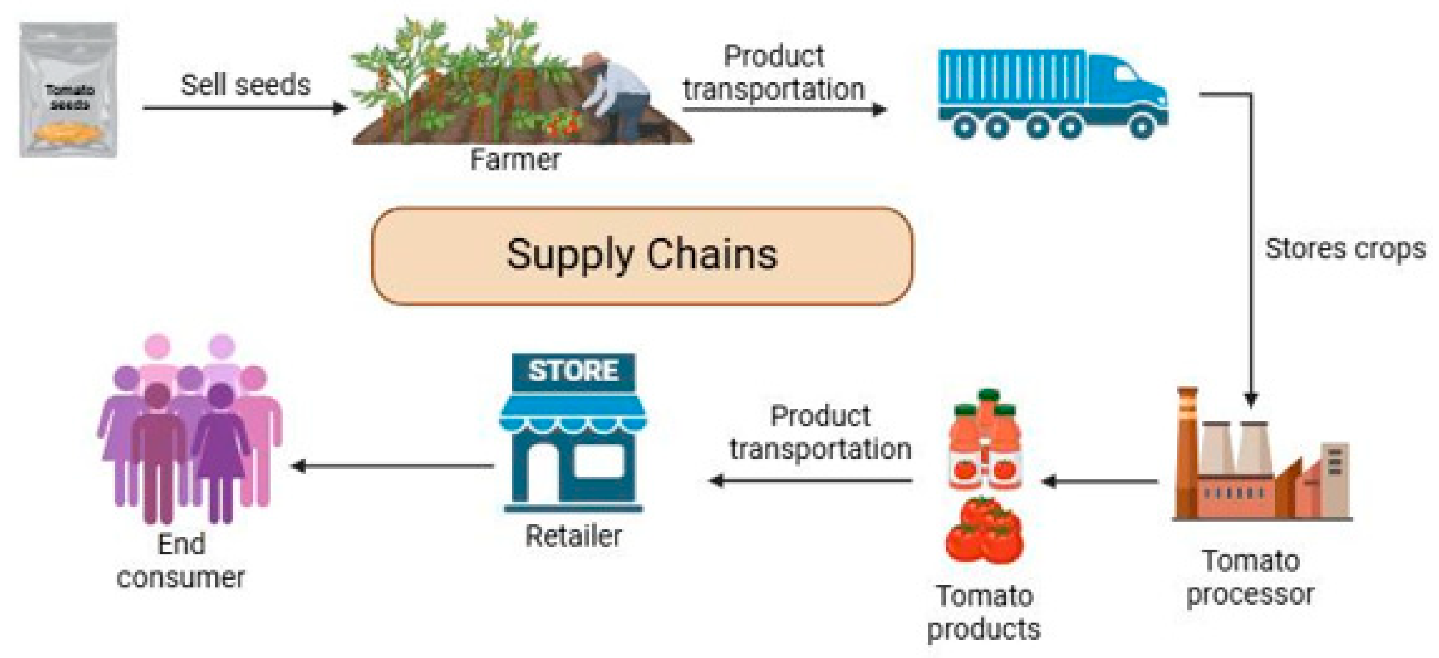
Figure 1. Generic tomato supply chain.
World 06 00129 g001
Figure 2. High volume tomato production from 2010 to 2023 in Sinaloa, México.
World 06 00129 g002
Figure 3. Compartmental analysis description for AFTSC with a decrease.
World 06 00129 g003
Figure 4. Compartmental analysis description for an AFTSC with a decrease and reprocessing.
World 06 00129 g004
Figure 5. System 1 simulation description for the AFTSC with a decrease.
World 06 00129 g005
Figure 6. System 2 simulation description for an AFTSC with a decrease and reprocessing.
World 06 00129 g006
Table 1. Performance metrics for system 1 and system 2 (sustainability and production).
System DynamicsSustainability IndexProduction (MT)
System 1 η 1 = 26.6 % W I P 1 = 2200
System 2 η 2 = 43.7 % W I P 2 = 500
Table 2. Simulation parameters for system 1.
DescriptionParametersUnits
Capacity for producers 1 C 11 500 MT
Capacity for distributors 1 C 21 400 MT
Capacity for customers 1 C 31 3000 MT/day
Dissipation rate echelon 1 γ 1 3 MT/day
Dissipation rate echelon 2 γ 2 2.5 MT/day
Dissipation rate echelon 3 γ 3 2 MT/day
Production rate echelon 1–2 φ 12 25 MT/day
Production rate echelon 2–3 φ 23 22 MT/day
Throughput y 1 1.5 MT/day
Demand rate u 1 5000 MT/day
Table 3. Simulation parameters for system 2.
DescriptionParametersUnits
Capacity for producers 2 C 12 1500 MT
Capacity for distributors 2 C 22 1200 MT
Capacity for customers 2 C 32 1000 MT
Capacity for reprocessing 1 C 42 800 MT
Capacity for reprocessing 2 C 52 600 MT
Dissipation rate echelon 1 γ 1 4.5 MT/day
Dissipation rate echelon 2 γ 2 3.8 MT/day
Dissipation rate echelon 3 φ 12 20 MT/day
Production rate echelon 1-2 φ 23 15 MT/day
Production rate echelon 2-3 ζ 11 8.9 MT/day
Reprocessing rate echelon 1-1 ζ 12 6 MT/day
Reprocessing rate echelon 1-2 ζ 21 9.5 MT/day
Reprocessing rate echelon 2-2 ζ 22 12 MT/day
Reprocessing rate echelon 3-3 ζ 32 11 MT/day
Throughput system 2 y 2 5 MT/day
Demand rate system 2 u 2 3000 MT/day
Disclaimer/Publisher’s Note: The statements, opinions and data contained in all publications are solely those of the individual author(s) and contributor(s) and not of MDPI and/or the editor(s). MDPI and/or the editor(s) disclaim responsibility for any injury to people or property resulting from any ideas, methods, instructions or products referred to in the content.