Abstract
Groundwater is essential for irrigated agriculture, yet its use remains unsustainable in many regions worldwide. In countries like Pakistan, the situation is particularly pressing. The irrigated agriculture of Pakistan heavily relies on groundwater resources owing to limited canal-water availability. The groundwater quality in the region ranges from good to poor, with the lower-quality water adversely affecting soil structure and plant health, leading to reduced agricultural productivity. The delineation of quality zones with respect to irrigation parameters is thus crucial for optimizing its sustainable use and management. Therefore, this research study was carried out in the Lower Chenab Canal (LCC) irrigation system to assess the spatial distribution of groundwater quality. The geostatistical analysis was conducted using Gamma Design Software (GS+) and the Kriging interpolation method was applied within a Geographic Information System (GIS) framework to generate groundwater-quality maps. Semivariogram models were evaluated for major irrigation parameters such as electrical conductivity (EC), residual sodium carbonate (RSC), and sodium adsorption ratio (SAR) to identify the best fit for various Ordinary Kriging models. The spherical semivariogram model was the best fit for EC, while the exponential model best suited SAR and RSC. Overlay analysis was performed to produce combined water-quality maps. During the pre-monsoon season, 17.83% of the LCC area demonstrated good irrigation quality, while 42.84% showed marginal quality, and 39.33% was deemed unsuitable for irrigation. In the post-monsoon season, 17.30% of the area had good irrigation quality, 44.53% exhibited marginal quality, and 38.17% was unsuitable for irrigation. The study revealed that Electrical Conductivity (EC) was the primary factor affecting water quality, contributing to 71% of marginal and unsuitable conditions. In comparison, the Sodium Adsorption Ratio (SAR) accounted for 38% and Residual Sodium Carbonate (RSC) contributed 45%. Therefore, it is recommended that groundwater in unsuitable zones be subjected to artificial recharge methods and salt-tolerated crops to enhance its suitability for agricultural applications.
Keywords:
agriculture; geostatistics; groundwater; Kriging; GIS; semivariogram; Gamma Design Software (GS+) 1. Introduction
Successful agricultural practices are closely linked to a reliable water supply that fulfills the water requirements of crops. In regions where surface water supply and precipitation are inadequate, groundwater functions as an alternative resource to sustain high agricultural productivity, contingent upon its acceptable quality. Globally, approximately 112 million hectares of land are irrigated using groundwater, with countries such as the USA, India, Pakistan, and China accounting for more than 70% of the world’s groundwater-irrigated area [1,2]. Worldwide, approximately 60% of crop grain production comes from irrigated agriculture, which consumes two-thirds of the freshwater that is withdrawn from groundwater-figures that have remained relatively consistent over the past two decades, as reported by FAO and UNESCO. Annually, approximately 1000 billion cubic meters of groundwater are extracted globally for irrigated agriculture, with this volume continuing to rise due to increasing agricultural demands [3,4].
Pakistan heavily depends on irrigated agriculture due to its predominantly arid and semi-arid climate. Approximately 20 million hectares of land are cultivated, with key crops including wheat, rice, cotton, and sugarcane, all of which rely significantly on supplemental groundwater resources [5,6]. Agriculture contributes about 19–20% of GDP and employs nearly 38% of the labor force. Groundwater accounts for 40–50% of Pakistan’s irrigation water supplies, especially during canal shortages and dry seasons. Driven by a growing population and increasing demand for food production, over 1.5 million tubewells are currently in operation in Pakistan, extracting approximately 65 billion cubic meters of groundwater annually, with more than 90% being utilized for agricultural irrigation [7]. The prolonged over-extraction of groundwater at rates exceeding natural recharge has led to a significant decline in groundwater levels. Furthermore, the lateral intrusion of saline groundwater from neighboring areas has deteriorated the quality of fresh groundwater in various parts of the Indus Plain, causing groundwater to become more saline [8]. Moreover, for irrigation, the application of groundwater of poor quality in the regions of irrigated agriculture is considered one of the significant causes of salinity, resulting in reduced food productivity [9,10]. Secondary salinization in Punjab, Pakistan, caused using saline groundwater for irrigation, has led to significant agricultural and environmental challenges. Crop yields, such as wheat and rice, have dropped by 30–40% and 25–35%, respectively, due to high salt levels in the soil and water. Around 20–25% of irrigated land is now moderately to severely saline, with soil fertility declining as organic matter decreases by 15–20%. Farmers in affected areas face income losses of 40–50% due to lower yields and higher costs for soil restoration. Additionally, groundwater in these regions often has an Electrical Conductivity (EC) of 3–6 dS/m, well above the safe limit of 1 dS/m for irrigation. These issues highlight the urgent need for better water-management and soil-reclamation practices [11]. Excessive sodium in the soil can damage its structure, reducing air circulation, water absorption, and permeability, which negatively affects plant growth [12,13,14].
Mapping the spatial distribution of groundwater quality is essential for informed resource management, enabling targeted interventions, optimized irrigation practices, and the sustainable utilization of groundwater across varying hydrogeological zones. Geographical Information System (GIS) is a substantial tool for spatial data assessment and water-quality mapping using geostatistics [15,16]. Geostatistical analysis, combined with advanced spatial interpolation techniques like Kriging, provides a robust framework for assessing groundwater quality and quantity [17,18,19,20,21]. Kriging is widely used over other interpolation methods such as Inverse Distance Weighting (IDW) and spline because it accounts for spatial autocorrelation and provides both prediction values and associated error estimates [22,23,24]. By delineating groundwater zones, policymakers and farmers can make informed decisions about water-resource management, ensuring sustainable agricultural practices. Despite its potential, the application of geostatistical methods in groundwater zoning for irrigated agriculture remains underexplored in many regions, particularly in developing countries.
The lack of precise and spatially explicit groundwater quality and availability data hinders effective water-resource management for irrigated agriculture [3,25,26]. Traditional methods of groundwater assessment are often inadequate for capturing spatial variability, resulting in inefficient irrigation practices and resource mismanagement. There is an urgent need to employ advanced geostatistical techniques to delineate groundwater zones and assess their suitability for irrigation. Thus, this study aims to apply geostatistical analysis techniques to assess the spatial distribution of key groundwater-quality parameters in the Lower Chenab Canal region, with the aim of delineating irrigation suitability zones and supporting sustainable agricultural water management.
2. Research Site
The Lower Chenab Canal (LCC) irrigation circle was selected as the research site for this study, situated in the central-eastern region of Punjab, Pakistan. The LCC is positioned between longitudes 73°39′19″ E and 72°18′54″ E, and latitudes 32°16′14″ N and 30°45′53″ N, illustrated in Figure 1. The canal’s command area covers 1.8228 million hectares (18,228 square kilometers) and is situated at the core of the Rechna Doab sub-basin, which lies between the Ravi and Chenab rivers. The irrigation system of LCC in Punjab was structured from 1892 to 1898 through the era of British colonialism [27]. The main cities of the study area are Toba Tek Singh, Hafizabad, and Faisalabad. The study area is further divided into seventeen (17) irrigation subdivisions which are Sagar, Sangla, Chuharkana, Mohallan, Paccadalla, Kot Khudayar, Uqbana, Buchiana, Tandianwala, Kanya, Tarkhani, Aminpur, Veryam, Wer, Dhaular, Bhagat, and Sultanpur.
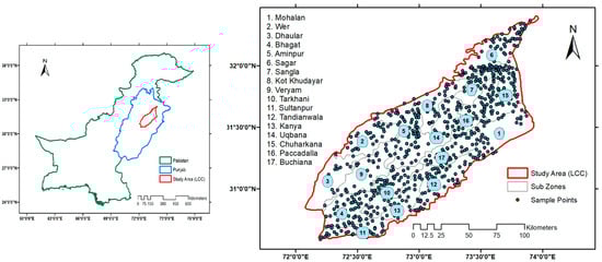
Figure 1.
Location of wells (sample points) and irrigation subzones of LCC.
The River Chenab flows along the northern boundary of the area, moving from northeast to southwest, and it passes through the Khanki, Qadirabad, and Trimmu headworks/barrages, which define the study area’s limits (Figure 2). The Jhang Branch Canal serves as an irrigation canal, while the Qadirabad Baloki and Trimmu Sidhnai canals act as link canals, both flowing from the northwest to the southeast through the study area. The soils in the study area consist of alluvial deposits transported by the Indus River and its tributaries. The surface soils’ textures are predominantly fine and moderately medium, with favorable permeability characteristics and are similar throughout the area.
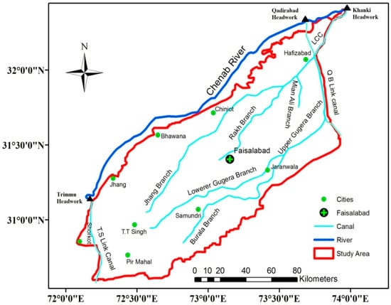
Figure 2.
Canal networks in research area.
Climate
The study area exhibits climatic variation, with the southwest generally classified as semi-arid and the northeast as sub-humid. According to the Köppen–Geiger climate classification, Hafizabad falls under a hot semi-arid climate (BSh), while Toba Tek Singh is characterized by a hot desert climate (BWh). Rainfall and temperature are the most essential parameters for determining the climatic conditions with great seasonal fluctuations. In the monsoon season (July to September), maximum rainfall is observed. The mean yearly rainfall in the study area is recorded as 427 mm. The summer season is commonly hot from May to September. The min. temperature is 21 °C and the maximum temperature is 49 °C in summer. The winter season remains from November to February. The minimum temperature is 6 °C and the maximum temperature is 25 °C in winter. The nature of the soil in LCC is basic because the pH value is in the range of 8 to 8.5. Medium-to-fine sand, silt, and clay exist in the upper side of LCC as an excessive percentage and they are homogeneously spread, while clay, in greater amounts, is found just in depression regions [28,29].
3. Materials and Methods
3.1. Data Collection
Various chemical indices have been used by scientists, including electrical conductivity (EC), residual sodium carbonate (RSC), and sodium absorption ratio (SAR) to comprehend groundwater quality for irrigation [30,31]. High Sodium Adsorption Ratio (SAR) can worsen soil compaction, lower water infiltration, and hinder crop growth due to increased sodium levels [32,33]. Over time, without proper leaching, sodium can build up in the soil, causing harm to both soil health and crop productivity. To combat salinity problems, experts recommend planting salt-tolerant plants (halophytes) alongside effective soil-management practices [34]. Water-quality samples were collected from 747 wells across the study area during the pre-monsoon (June) and post-monsoon (October) seasons of 2022. The well locations were strategically selected to ensure spatial representativeness, covering a range of hydrogeological zones, to effectively capture the spatial variability of groundwater quality. The water samples were taken from each well using clean plastic bottles once the water flow had stabilized. These samples were first tested for electrical conductivity (EC) on-site using a calibrated EC meter (TDS-98302). Later, the Sodium Adsorption Ratio (SAR) and Residual Sodium Carbonate (RSC) were measured in the Water Quality Testing Lab at the Department of Agricultural Engineering, Bahauddin Zakariya University, Multan-Pakistan, following the standard method outlined in the USDA Agriculture Handbook 60. Usually, problems related to the utilization of poor groundwater quality are sodicity, alkalinity, toxicity, and salinity [24]. The water-quality parameters used in this study, along with their classification for irrigation purposes, are presented in Table 1. Statistical analysis, including the minimum, maximum, mean values, and standard deviations of each parameter, was performed. Additionally, the Pearson correlation matrix was computed using Statistix 8.1 software to assess the linear relationships among the water-quality parameters.

Table 1.
Water-quality standards.
3.2. Groundwater-Quality Mapping
Figure 3 outlines the methodological workflow, structured in three main steps: data preparation, variogram modeling, and suitability mapping. Each step involves systematic procedures from data collection to spatial analysis using Kriging, classification of maps, and overlay analysis for final maps. The individual components of each step are described in detail below.
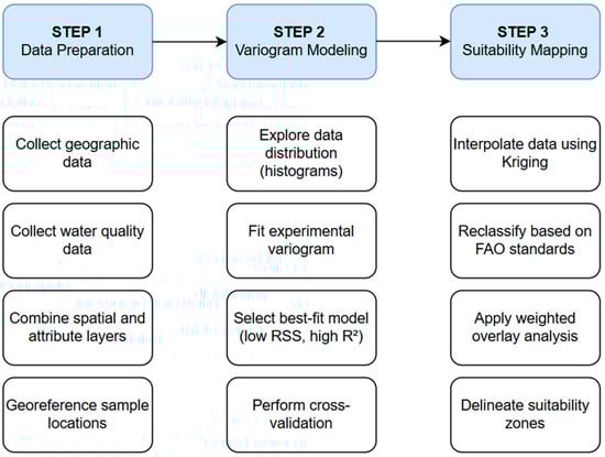
Figure 3.
Flow chart to create water-quality maps.
3.3. Geostatistics
Data interpolation at various unsampled points was carried out using geostatistical techniques. There are two main approaches to data interpolation: deterministic and geostatistical [36]. The geostatistical approach, particularly Kriging, is considered the most suitable as it incorporates probability in data predictions. For the geostatistical analysis, Gamma Design Software (GS+, version 10) was employed, while ArcGIS 10.1 was used for groundwater mapping. ArcGIS has advanced geostatistical tools, a user-friendly interface, and seamless integration with other software, making it ideal for spatial data analysis and mapping. The Geostatistical Analyst extension provides robust interpolation techniques like Kriging, essential for modeling groundwater-quality parameters [37,38]. Compared to platforms like QGIS or GRASS GIS, ArcGIS 10.1 offers superior scalability, flexibility, and visualization capabilities, enabling efficient handling of large datasets and high-quality map production. Its reliability, extensive documentation, and technical support further enhance its suitability for this research [39,40,41].
3.4. Semivariogram
To determine the spatial autocorrelation and similarity of data within the study area, a semivariogram measures the degree of divergence among unsampled and adjacent locations. A graph of the semivariogram is obtained by incorporating semivariogram values at various lag distances. The semivariogram models (linear, spherical, circular, exponential, and Gaussian) give information about which semivariogram model is the best-fit model for Kriging interpolation and describe the spatial autocorrelation analysis of data [42,43]. The value at which the semivariogram intercepts the y-axis is referred to as the nugget. The value at which the semivariogram model reaches its maximum on the y-axis is termed the sill. In a semivariogram, the lag distance at which the model curve becomes nearly horizontal and remains constant is defined as the range [44].
3.5. Kriging
Kriging interpolation is a method employed for estimating groundwater-quality data at various unsampled locations. The accuracy of the estimates produced by this technique relies heavily on the theoretical variogram model and the spatial distribution of the observed data points [16]. Various types of Kriging interpolation, i.e., simple, ordinary, and universal Kriging, exist in the literature. Ordinary Kriging is the most appropriate geostatistical method for areas where the values of neighboring data points exhibit greater similarity compared to those that are farther apart [45]. To perform Kriging, it is necessary to check normal distribution of data and spatial dependence through histogram and semivariogram analysis [46].
3.6. Cross-Validation
Cross-validation is applied to validate the accuracy of estimations and assess the suitability of semivariogram models [47]. To evaluate the performance of the interpolation models, metrics such as mean error (ME), root mean square error (RMSE), and average standard error (ASE) were calculated using Equations (1)–(3), respectively, adoptive from [48].
Here, N = number of observations, = observed value, = predicted value, and Kriging variance for location . The value of ME should be approximately zero for good predictions [47]. The lower values of the RMSE and ASE errors indicate a better prediction of interpolation models [16,49]. ME, RMSE, and ASE were selected as performance metrics for cross-validation because they collectively evaluate bias, accuracy, and uncertainty in geostatistical models like Kriging. Mean error (ME) assesses systematic bias, ensuring predictions are not consistently over- or underestimated. Root mean square error (RMSE) measures overall accuracy, penalizing larger errors and making it sensitive to outliers, which is critical for groundwater-quality datasets. Average standard error (ASE) evaluates the model’s confidence by comparing predicted uncertainty to RMSE, ensuring reliable uncertainty estimates. While other metrics like MAE or R2 exist, they lack sensitivity to outliers or can be misleading in spatially autocorrelated data. ME, RMSE, and ASE provide a balanced assessment, making them ideal for groundwater zoning studies aimed at sustainable agricultural planning [22,50,51].
3.7. Reclassification and Overlay
The maps of groundwater quality were prepared through the Kriging method according to the criteria of FAO. Further, these maps were reclassified, and every class was given a single value. The class that shows good quality is assigned by high value and unsuitable quality is assigned by low value. The weighted sum overlay is a technique in which each layer of water-quality parameters is incorporated into a single combined layer with weights of 9 for Good, 9–6 for Marginal, and <6 for Unsuitable quality to assess the potential of groundwater-quality regions and prepare final maps for the pre-monsoon and post-monsoon seasons.
4. Results and Discussion
4.1. Analysis of Groundwater-Quality Parameters
Descriptive statistical analysis of water-quality data to appraise the preliminary groundwater quality is demonstrated in Table 2 for the season of pre-monsoon (June) and post-monsoon (October). The values of minimum, mean, maximum, and standard deviation (SD) are described as a statistical summary. Electrical conductivity (EC) values remained relatively stable across seasons, with mean values of 2.20 dS/m (pre-monsoon) and 2.18 dS/m (post-monsoon). The observed range was narrow, from 0.66 to 8.48 dS/m pre-monsoon and 0.69 to 8.23 dS/m post-monsoon.
Table 2.
Statistics of groundwater-quality parameters.
The mean Sodium Absorption Ratio (SAR) values were 9.63 for the pre-monsoon season and 8.68 for the post-monsoon season, showing some variation, though the overall water quality remained satisfactory during both seasons. Additionally, the maximum value of Residual Sodium Carbonate (RSC) observed in the pre-monsoon season was 7.43 meq/L, which rose to 13.10 meq/L during the post-monsoon season. A slight variation in minimum values of RSC was recorded from 0.00 to 0.04 meq/L. Pearson correlation coefficients were calculated to assess the strength and direction of linear relationships among groundwater-quality parameters, and the results are presented in Table 3. The Pearson correlation matrix shows a strong positive correlation between EC_JUNE and EC_OCT (r = 0.96), indicating seasonal consistency in salinity levels. SAR_JUNE is also strongly correlated with SAR_OCT (r = 0.90), suggesting similar sodicity patterns across seasons. RSC_JUNE and RSC_OCT exhibit a very strong relationship (r = 0.89), while RSC shows weak correlation with EC in both seasons (r ≈ 0.10), reflecting their distinct geochemical behaviors. Overall, SAR shows higher dependence on both EC and RSC, indicating its integrative nature.
Table 3.
Pearson correlation matrix.
Seasonal variation in groundwater quality is influenced by rainfall-driven dilution, excessive pre-monsoon pumping, and uneven recharge. Post-monsoon rainfall slightly reduced EC and SAR, while the increased RSC values may result from bicarbonate accumulation due to variable infiltration. These shifts reflect the interplay of hydrological and geochemical processes [39,52]. Groundwater quality in Punjab, Pakistan, has been widely studied, with EC ranging from 0.5 to 10 dS/m, indicating varying salinity levels [7,8,11,29]. SAR values range from 5 to 30, reflecting high sodicity risks in many areas, while RSC levels often exceed the safe limit of 2.5 meq/L, reaching up to 10 meq/L in some regions. These parameters highlight significant threats to agricultural productivity and water sustainability due to excessive irrigation and natural geogenic processes [11,52,53].
4.2. Histogram Analysis
Histogram analysis was employed to evaluate the normal distribution of the observed data. Several transformations, including Box–Cox and logarithmic transformations, were tested to verify the normality of the data [42]. Given that the observed water-quality parameters EC, SAR, and RSC exhibited positive skewness, a logarithmic transformation was applied to normalize the data, as shown in Figure 4. Compared to other transformations like Box–Cox, the logarithmic transformation is simpler to apply and interpret, especially when the data contains zero or negative values (which require adjustments in Box–Cox). Additionally, logarithmic transformation is particularly effective for datasets with a wide range of values, such as groundwater-quality parameters (e.g., salinity, nitrate concentrations), as it compresses the scale and reduces the influence of extreme values [42,43]. Recent studies [40,41] have demonstrated that logarithmic transformation outperforms other methods in normalizing environmental data, making it a preferred choice for geostatistical analysis.
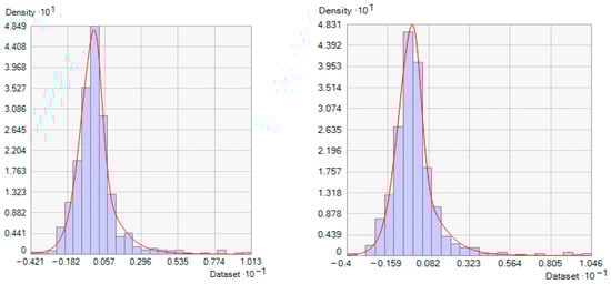
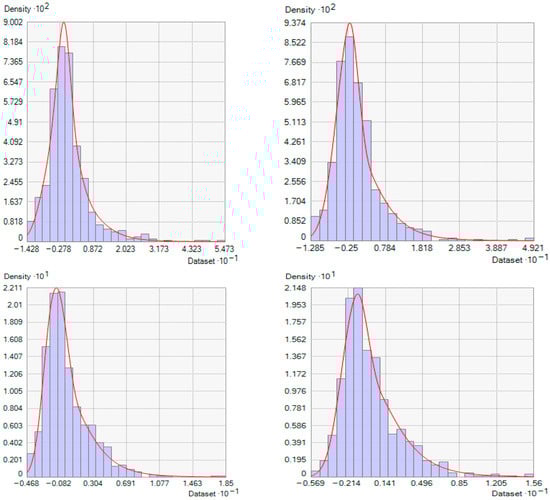
Figure 4.
Histogram graphs of the logarithmic normalized water-quality parameters.
4.3. Spatial Autocorrelation
The spatial structure of the variogram model was evaluated by comparing theoretical and experimental semivariograms using key metrics such as the coefficient of determination (R2), the residual sum of squares (RSS), and the nugget-to-sill ratio (Co/Co+C). The most suitable variogram model was determined based on the highest R2 and the lowest RSS values. For Electrical Conductivity (EC), the spherical model provided the best fit during the pre-monsoon season, while the exponential model was more appropriate for the post-monsoon season. In contrast, for the Sodium Absorption Ratio (SAR) and Residual Sodium Carbonate (RSC), the exponential model was identified as the best fit for both the pre-monsoon and post-monsoon seasons (Figure 5). The nugget-to-sill ratio indicates the spatial dependence of parameters, exhibiting an inverse relationship; a higher ratio signifies a weaker correlation among the parameters, while a lower ratio indicates a stronger correlation [54]. The values of R2 ranged from 0.491 to 0.816, while RSS values varied between 0.275 and 0.576.
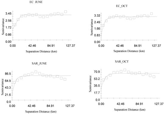
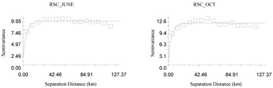
Figure 5.
Best-fitted semivariogram models for groundwater-quality parameters (spherical for EC_June and exponential for all others).
The spatial dependence of water-quality parameters is characterized by the nugget-to-sill ratio (Co/Co+C). A low ratio (<0.25 or below 25%) indicates strong spatial dependence, allowing for uniform management practices like consistent irrigation and fertilization across large areas. A moderate ratio (0.25–0.75 or 25–75%) signifies mixed influences from natural and human factors, necessitating zone-specific strategies such as targeted leaching or salt-tolerant crops in high-salinity zones. A high ratio (>0.75 or above 75%) reflects very weak spatial dependence, requiring site-specific interventions like frequent water testing and tailored irrigation to address localized variability. For example, in the Indo-Gangetic Plain, areas with low ratios enabled uniform irrigation, while high ratios demanded precise management to mitigate salinity [23,40]. Understanding this ratio helps optimize agricultural practices, ensuring sustainable water use and improved crop productivity. Table 4 shows that the water-quality parameters SAR and RSC for the pre-monsoon season and EC and RSC for the post-monsoon season have strong spatial dependence because the values of these parameters were found to be less than 25%. EC for pre-monsoon season and SAR for post-monsoon season has moderate spatial dependence due to it being found to be in the range of 25 to 75%. Ref. [55] identified the best-fitted semivariogram models for various groundwater-quality parameters and assessed their spatial dependence using the nugget-to-sill ratio, which ranged from 0% to 8%, indicating a strong spatial dependence in the data.
Table 4.
Results of semivariogram models for water-quality parameters.
4.4. Cross-Validation Results
The results of the performance of interpolation models such as mean error (ME), root mean square error (RMSE), mean square error (MSE), and average standard error (ASE) are presented in Table 5, with ME values ranging from −0.0229 to 0.1676, RMSE values from 1.4572 to 8.0727, ASE values from 1.2489 to 9.2068, and MSE values from −0.0153 to 0.0093. The ME values being close to zero indicate that the interpolation model provides better predictions. A negative ME value indicates that the model’s predicted values are greater than the observed values. Lower ASE and RMSE values suggest minimal and acceptable prediction errors for the interpolation model. Ref. [47] also applied the cross-validation technique to verify the accuracy of estimations and the appropriateness of the semivariogram models.
Table 5.
Statistical outcomes of cross-validation of EC, SAR, and RSC.
4.5. Delineation Groundwater Quality
4.5.1. Electrical Conductivity (EC)
Figure 6 presents the analysis and variation of electric conductivity across the different irrigation sub-zones, where dark blue represents good quality, light yellow indicates marginal quality, and light rose denotes unsuitable groundwater status. The Kot Khudayar irrigation subdivision experienced the largest increase (4.96%) in areas classified as having good groundwater quality based on EC values. Conversely, the Wer irrigation subdivision saw the highest reduction (9.94%) in good groundwater quality. After the monsoon season, the Buchiana irrigation subdivision recorded the largest increase (14.92%) in areas classified as marginal. However, Kot Khudayar also saw a reduction in the area under marginal groundwater quality (4.69%). The Buchiana subdivision had the greatest reduction in areas classified as unsuitable quality (15.41%), while Uqbana experienced the largest increase (3.65%) in this category (Table 6).
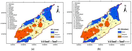
Figure 6.
Delineation of Electrical Conductivity (EC) across various subzones (June) (a) pre-monsoon; (b) post-monsoon (October).
Table 6.
Variation in groundwater quality across different sub-zones in October compared to June.
High pumpage of groundwater and less recharge in the study area can also result in a high percentage of salinity [11,31]. The western part of the Lower Chenab Canal (LCC) exhibits lower salinity levels due to the presence of an extensive river belt and greater recharge, as reported by [30,56]. In contrast, the eastern part of the LCC shows higher salinity levels, attributed to reduced rainfall and lower recharge in that region.
4.5.2. Sodium Absorption Ratio (SAR)
Figure 7 presents a detailed subdivisional investigation and variation in SAR, where blue indicates good quality, light green represents marginal quality, and orange denotes unsuitable groundwater conditions across different subzones. The Kanya irrigation subdivision experienced an improvement in groundwater quality, with 26.86% of the area classified as good quality (Figure 7), while the Bhagat subdivision witnessed a decline of 21.64% in the area categorized as good quality, although it also saw an increase in marginal groundwater quality, which now encompasses 12.94% of the area. Most of the areas under the marginal category decreased following the monsoon season. Notably, unsuitable water quality decreased in nearly all subdivisions, except for Bhagat, which observed an increase of 8.70% in areas classified as unsuitable after the monsoon. Spatial distribution describes how some central regions of LCC have higher concentrations of SAR for both seasons. In the case of SAR, most of the areas around the northeastern, northwestern, and southern parts are of good water quality. The remaining area of LCC has marginal groundwater quality. Alkalinity is a less important problem as compared to salinity in the study area.
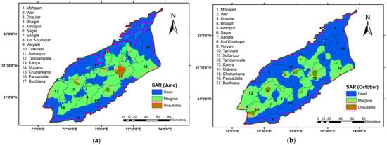
Figure 7.
Delineation of Sodium Absorption Ratio (SAR) across various subzones (a) pre-monsoon (June); (b) post-monsoon (October).
The SAR in groundwater tends to change notably because of the extra water from rainfall and surface runoff. Research also shows that SAR levels often drop right after the monsoon, as the added freshwater dilutes sodium more than calcium and magnesium. However, in areas with a lot of farming, SAR can increase later in the season as salts and fertilizers seep into the groundwater [57,58]. These changes matter for irrigation because high SAR can harm soil quality, making it less suitable for farming [59]. The sodium concentration appearing in excess amounts, as compared to calcium and magnesium, in irrigation water decreases the soil permeability, thereby restricting the water supply to the plants [60].
4.5.3. Residual Sodium Carbonate (RSC)
Figure 8 illustrates a detailed subdivisional investigation and variation in groundwater quality based on RSC, where purple represents good quality, light yellow indicates marginal quality, and orange denotes unsuitable groundwater conditions across different subzones. The Sangla irrigation subdivision experienced an increase of 11.39% in the area classified as good quality; however, there was an unexpected decrease in good quality following the monsoon. In the Bhagat subdivision, the area under marginal quality increased by 12.08%, while the remaining irrigation subdivisions exhibited a decline in groundwater quality. Notably, all irrigation subdivisions experienced an increase in unsuitable quality after the monsoon, with the largest areas affected being 24.75% in the Chuharkana subdivision and 22.35% in the Tarkhani subdivision. The deterioration in groundwater quality in Southern areas such as Bhagat may be driven by intensive groundwater pumping and possible saline water intrusion, compounded by limited recharge due to reduced canal flow and significantly lower rainfall compared to the northern sub-regions. For instance, The Toba Tek Singh district (Bhagat) receives approximately 350 mm of annual precipitation, whereas the Northern part (Hafizabad) averages around 550 mm per year [61]. RSC exhibited greater spatial variation than SAR and EC due to its sensitivity to localized geochemical processes, soil characteristics, and anthropogenic activities. Carbonate and bicarbonate ions, which influence RSC, vary significantly with weathering, agricultural practices, and recharge rates, while SAR and EC are more stable [62]. Similar findings were reported in studies from Delhi and the Indus Basin, where RSC showed higher variability due to carbonate-rich soils and irrigation impacts. Using ArcGIS and geostatistical tools, these variations were effectively mapped, highlighting the importance of RSC in groundwater-quality assessment for irrigated agriculture [9,40,63]. Ref. [64] described how the successive application of water with too much RSC cannot allow the movement of water and air through the soil and this deteriorates the structure of the soil, thereby decreasing the yield of crops. Higher values of RSC depict the hazard of sodicity. Soil particles can absorb sodium (Na) if water has high values of RSC [65]. Ref. [66] analyzed the hazardous impacts of carbonate and bicarbonate in terms of residual sodium carbonate on crops and soil health. The percent area of LCC in the case of RSC under unsuitable water quality is less as compared to that of EC and SAR.
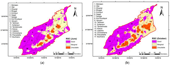
Figure 8.
Delineation of Residual Sodium Carbonate (RSC) across various subzones: (a) pre-monsoon (June); (b) post-monsoon (October).
4.6. Overall Groundwater Quality
Individual classified layers of water-quality parameters were reclassified to create a single composite layer using the Weighted Sum technique of overlay analysis as shown in Figure 9. Water-quality ratings and color were assigned as follows: 9 for good quality (dark green), 6–8 for marginal quality (yellow), and values less than 6 for unsuitable (red) groundwater quality. Table 7 presents the distribution of the reclassified values and the area under various water-quality categories, detailing the overall groundwater quality for the Lower Chenab Canal (LCC) study area. During the pre-monsoon season, an area of 3249.46 km2 (17.83%) in the LCC was classified as having good-quality irrigation water; however, this unexpectedly decreased to 3153.62 km2 (17.30%) in the post-monsoon season. An area of 7808.93 km2, representing 42.84%, was categorized as having marginal-quality irrigation water during the pre-monsoon season, while this figure rose to 8117.17 km2 (44.53%) in the post-monsoon season. The area classified as unsuitable quality was found to be 7169.33 km2 (39.33%) during the pre-monsoon season and decreased to 6956.74 km2 (38.17%) during the post-monsoon season. These trends align with findings from [38,58,67], which highlight seasonal variations in groundwater quality due to monsoonal influences, such as dilution and recharge processes. The excessive use of fertilizers and pesticides in agriculture are among the primary factors affecting the quality of groundwater for drinking and agriculture purposes [59]. The geological composition of the study area, predominantly comprising alluvial deposits from the Indus River system, plays a significant role in shaping groundwater chemistry by influencing the dissolution of salts and bicarbonates. Variations in crop type such as rice and sugarcane in the northeast (Hafizabad) and cotton and wheat in the southwest (Toba Tek Singh) may also affect spatial differences in SAR and RSC, as intensive irrigation and fertilizer use contribute to chemical loading and recharge quality.
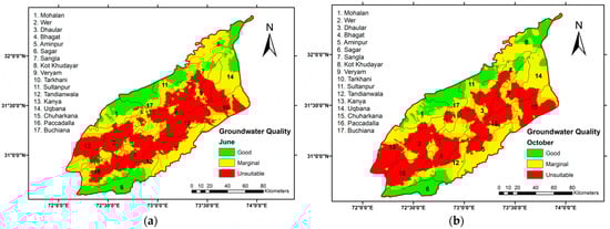
Figure 9.
Overall groundwater-quality maps generated from overlay analysis: (a) pre-monsoon (June); (b) post-monsoon (October).
Table 7.
The area covered by different quality categories and re-class values.
Furthermore, the findings of this study are also consistent with previous research in the Indus Basin and other semi-arid regions where groundwater salinity and sodicity pose significant threats to agricultural productivity. For instance, Refs. [8,10,11] have reported widespread groundwater degradation due to excessive abstraction and inadequate recharge in Punjab, aligning with the observed spatial variability in EC, SAR, and RSC across the LCC area. The spatial dependence patterns derived from semivariogram analysis also correspond with the work of [29,30], who found similar results regarding moderate-to-strong spatial autocorrelation in groundwater-quality parameters using geostatistical methods. However, while previous studies primarily focused on salinity (EC), this study provides a more integrated assessment by incorporating SAR and RSC, enabling a nuanced classification of irrigation suitability zones. Despite this contribution, a notable gap remains in the inclusion of major ions (e.g., Na+, Ca2+, Mg2+, Cl−, HCO3−, and SO42−), which are critical to understanding the hydrochemical evolution of groundwater and its long-term impacts on soil health. Future studies should aim to integrate comprehensive hydrochemical datasets with geostatistical and hydrogeological models to better understand contaminant sources, predict trends, and support adaptive management strategies under changing climatic and land-use conditions.
5. Conclusions
Based on the evaluation of spatial groundwater quality, several conclusions are drawn from this study: the spherical model best fit EC data in the pre-monsoon season, while the exponential model performed better post-monsoon. For SAR and RSC, the exponential model was determined to be the optimal fit for both seasons. The results of the cross-validation indicated that the values of the best-fit semivariogram model fell within acceptable limits. Selecting the best-fit semivariogram models, such as spherical for EC and exponential for SAR and RSC, improves spatial-prediction accuracy and supports reliable groundwater-quality zoning for effective field-level irrigation management. Most areas in terms of salinity in LCC were classified as marginal-quality groundwater. The largest unsuitable area concerning EC was identified in the Veryam irrigation subdivision. The Sodium Absorption Ratio (SAR) values indicate that the Lower Chenab Canal (LCC) area was less impacted by alkalinity relative to salinity and sodicity. Groundwater sodicity, indicated by RSC, was less prevalent than salinity but more significant than alkalinity. The highest unsuitable areas were observed in the Paccadalla subdivision, covering 30.84% (pre-monsoon) and 35.24% (post-monsoon). According to the overlay analysis, the overall good-quality groundwater constituted 17.83% of the LCC area during the pre-monsoon season and 17.30% during the post-monsoon season. Marginal-quality groundwater accounted for 42.84% and 44.53% of the area in the respective seasons. The area classified as unsuitable quality was recorded at 39.33% for the pre-monsoon season and 38.17% for the post-monsoon season.
The challenges of groundwater quality in the Lower Chenab Canal (LCC) area should be addressed by engaging stakeholders and policymakers. In high-salinity zones and areas with poor pre-monsoon water quality, crop rotation with salt-tolerant varieties such as barley and sorghum, along with water-saving strategies and precision agriculture, is recommended. In contrast, regions showing improved post-monsoon water quality are better suited for water-intensive crops and leaching practices to enhance soil conditions. Infrastructure such as recharge wells, percolation tanks, and check dams should be developed to enhance aquifer recharge, alongside enforcing groundwater-extraction regulations to prevent overexploitation. Regular water-quality monitoring and farmer training programs on sustainable practices are essential, as is investing in research for salt-tolerant crops. Designating buffer zones around high-quality areas and fostering public–private partnerships for large-scale projects will further ensure long-term groundwater sustainability.
However, this research work has certain limitations. Data-collection challenges, such as inconsistent monitoring and limited spatial coverage, may affect the accuracy of groundwater-quality assessments. The application of geostatistical models, while effective, relies on assumptions about spatial variability that may not fully capture localized anomalies. Future studies could benefit from higher-resolution data, the integration of remote sensing, and a groundwater modeling study to address these limitations and enhance the reliability of the findings. By leveraging these insights, stakeholders can implement data-driven irrigation practices, improve agricultural productivity, and ensure the sustainable use of groundwater resources in the LCC area.
Author Contributions
Conceptualization, A.S. and M.N.S.; methodology, I.R.; software, A.T.O. and H.U.F.; validation, H.A.K., A.Q.B. and A.A.K.; formal analysis, A.S. and M.N.S.; investigation, A.T.O.; resources, M.S.R.; data curation, I.R. and H.U.F.; writing—original draft preparation, A.S., A.Q.B. and M.N.S.; writing—review and editing, S.A.S.; visualization, A.T.O. and H.A.K.; supervision, S.A.S. and A.T.O.; project administration, A.A.K.; funding acquisition, S.A.S. All authors have read and agreed to the published version of the manuscript.
Funding
This research is supported by the Northwest Institute of Eco-environmental and Resource, Chinese Academy of Sciences, Lanzhou China through project no. (E539880106).
Institutional Review Board Statement
Not applicable.
Informed Consent Statement
Not applicable.
Data Availability Statement
All the data is available from the corresponding author.
Acknowledgments
The authors are grateful to the Northwest Institute of Eco-environment and Resource, Chinese Academy of Sciences, Lanzhou, China; Bahuddin Zakariya University, Multan; Pakistan, National University of Technology, Islamabad, Pakistan; and Aror University of Art, Architecture, Design and Heritage, Sindh, Sukkur, Pakistan for providing resources and support.
Conflicts of Interest
The authors declare no conflicts of interest.
References
- Siebert, S.; Burke, J.; Faures, J.M.; Frenken, K.; Hoogeveen, J.; Döll, P.; Portmann, F.T. Groundwater use for irrigation—A global inventory. Hydrol. Earth Syst. Sci. 2010, 14, 1863–1880. [Google Scholar] [CrossRef]
- FAO. The State of Food and Agriculture 2021: Making Agrifood Systems More Resilient to Shocks and Stresses. Available online: https://www.fao.org/publications/sofa/2021/en/ (accessed on 19 April 2022).
- Famiglietti, J.S. The global groundwater crisis. Nat. Clim. Change 2014, 4, 945–948. [Google Scholar] [CrossRef]
- UNESCO. The United Nations World Water Development Report 2022: Groundwater: Making the Invisible Visible. Available online: https://unesdoc.unesco.org/ark:/48223/pf0000380721 (accessed on 4 October 2023).
- Qureshi, A.S.; Gill, M.A.; Sarwar, A. Sustainable groundwater management in Pakistan: Challenges and opportunities. Irrig. Drain. J. Int. Comm. Irrig. Drain. 2010, 59, 107–116. [Google Scholar] [CrossRef]
- Javed, Q.; Arshad, M.; Bakhsh, A.; Shakoor, A.; Chatha, Z.A.; Ahmad, I. Redesigning of drip irrigation system using locally manufactured material to control pipe losses for orchard. Land Water 2014, 13, 1–4. [Google Scholar]
- Lucy, L.; Ali, A.; Garthwaite, B.; Jehangir, F. Punthakey, and Basharat Saeed. 2021. “Groundwater in Pakistan’s Indus Basin: Present and Future Prospects.” World Bank, Washington, DC. Available online: http://documents.worldbank.org/curated/en/501941611237298661 (accessed on 4 October 2023).
- Basharat, M.; Tariq, A.U.R. Groundwater modelling for need assessment of command scale conjunctive water use for addressing the exacerbating irrigation cost inequities in LBDC irrigation system, Punjab, Pakistan. Sustain. Water Resour. Manag. 2015, 1, 41–55. [Google Scholar] [CrossRef]
- Qureshi, A.S.; McCornick, P.G.; Sarwar, A.; Sharma, B.R. Challenges and prospects of sustainable groundwater management in the Indus Basin, Pakistan. Water Resour. Manag. 2010, 24, 1551–1569. [Google Scholar] [CrossRef]
- Maas, E.V. Salinity and citriculture. Tree Physiol. 1993, 12, 195–216. [Google Scholar] [CrossRef]
- Qureshi, A.S.; McCormick, P.G.; Qadir, M.; Aslam, Z. Managing salinity and waterlogging in the Indus Basin of Pakistan. Agric. Water Manag. 2008, 95, 1–10. [Google Scholar] [CrossRef]
- Panneerselvam, B.; Muniraj, K.; Thomas, M.; Ravichandran, N.; Bidorn, B. Identifying influencing groundwater parameter on human health associate with irrigation indices using the Automatic Linear Model (ALM. In in a semi-arid region in India. Environ. Res. 2021, 202, 111778. [Google Scholar] [CrossRef]
- Karim, M.R.; Arham, M.A.; Shorif, M.J.U.; Ahsan, A.; Al-Ansari, N. GIS based geostatistical modelling and trends analysis of groundwater quality for suitable uses in Dhaka division. Sci. Rep. 2024, 14, 17449. [Google Scholar] [CrossRef]
- Shah, S.A.; Jehanzaib, M.; Kim, M.J.; Kwak, D.-Y.; Kim, T.-W. Spatial and temporal variation of annual and categorized precipitation in the Han River Basin, South Korea. KSCE J. Civ. Eng. 2022, 26, 1990–2001. [Google Scholar] [CrossRef]
- Delgado, C.; Pacheco, J.; Cabrera, A.; Batllori, E.; Orellana, R.; Bautista, F. Quality of groundwater for irrigation in tropical karst environment: The case of Yucatan, Mexico. Agric. Water Manag. 2010, 97, 1423–1433. [Google Scholar] [CrossRef]
- Mohammadpour, M.; Roshan, H.; Arashpour, M.; Masoumi, H. Machine learning assisted Kriging to capture spatial variability in petrophysical property modelling. Mar. Pet. Geol. 2024, 167, 106967. [Google Scholar] [CrossRef]
- Kaliyappan, S.P.; Hasher, F.F.B.; Abdo, H.G.; Sajil Kumar, P.J.; Paneerselvam, B. A Novel Integrated Approach to Assess Groundwater Appropriateness for Agricultural Uses in the Eastern Coastal Region of India. Water 2024, 16, 2566. [Google Scholar] [CrossRef]
- Hassan, W.; Raza, M.F.; Alshameri, B.; Shahzad, A.; Khalid, M.H.; Nawaz, M.N. Statistical interpolation and spatial mapping of geotechnical soil parameters of District Sargodha, Pakistan. Bull. Eng. Geol. Environ. 2023, 82, 37. [Google Scholar] [CrossRef]
- Burrough, P.A. GIS and geostatistics: Essential partners for spatial analysis. Environ. Ecol. Stat. 2001, 8, 361–377. [Google Scholar] [CrossRef]
- Rodell, M.; Famiglietti, J.S.; Wiese, D.N.; Reager, J.T.; Beaudoing, H.K.; Landerer, F.W.; Lo, M.H. Emerging trends in global freshwater availability. Nature 2018, 557, 651–659. [Google Scholar] [CrossRef]
- Shah, S.A.; Jehanzaib, M.; Park, K.W.; Choi, S.; Kim, T.-W. Evaluation and decomposition of factors responsible for alteration in streamflow in lower watersheds of the han river basin using different Budyko-based functions. KSCE J. Civ. Eng. 2023, 27, 903–914. [Google Scholar] [CrossRef]
- Li, J.; Heap, A.D. A review of comparative studies of spatial interpolation methods in environmental sciences: Performance and impact factors. Ecol. Inform. 2011, 6, 228–241. [Google Scholar] [CrossRef]
- Amini, H.; Ashrafzadeh, A.; Khaledian, M. Enhancing groundwater salinity estimation through integrated GMDH and geostatistical techniques to minimize Kriging interpolation error. Earth Sci. Inform. 2024, 17, 283–297. [Google Scholar] [CrossRef]
- Alshahrani, M.A.; Ahmad, M.; Laiq, M.; Nabi, M. Geostatistical analysis and multivariate assessment of groundwater quality. Sci. Rep. 2025, 15, 7435. [Google Scholar] [CrossRef] [PubMed]
- Usman, M.; Liedl, R.; Kavousi, A. Estimation of distributed seasonal net recharge by modern satellite data in irrigated agricultural regions of Pakistan. Environ. Earth Sci. 2015, 74, 1463–1486. [Google Scholar] [CrossRef]
- Shah, S.A.; Jehanzaib, M.; Yoo, J.; Hong, S.; Kim, T.-W. Investigation of the effects of climate variability, anthropogenic activities, and climate change on streamflow using multi-model ensembles. Water 2022, 14, 512. [Google Scholar] [CrossRef]
- Usman, M.; Hussain, E.; Rabbani, U.; Ghazi, S.; Irteza, S.M.; Gull, S. Spatiotemporal analysis of crop water requirements in Lower Chenab Canal (LCC) Irrigation System for the better management of water resources. Arab. J. Geosci. 2021, 14, 424. [Google Scholar] [CrossRef]
- Waqas, M.M.; Niaz, Y.; Ali, S.; Ahmad, I.; Fahad, M.; Rashid, H.; Awan, U.K. Soil salinity mapping using satellite remote sensing: A case study of Lower Chenab Canal system, Punjab. Earth Sci. Pak. 2020, 4, 07–09. [Google Scholar] [CrossRef]
- Shakoor, A.; Arshad, M.; Bakhsh, A.; Ahmed, R. GIS based assessment and delineation of groundwater quality zones and its impact on agricultural productivity. Pak. J. Agric. Sci. 2015, 52, 837–843. [Google Scholar]
- Adhikary, P.P.; Chandrasekharan, H.; Chakraborty, D.; Kamble, K. Assessment of groundwater pollution in West Delhi, India using geostatistical approach. Environ. Monit. Assess. 2010, 167, 599–615. [Google Scholar] [CrossRef]
- Chakraborty, B.; Roy, S.; Bera, B.; Adhikary, P.P.; Bhattacharjee, S.; Sengupta, D.; Shit, P.K. Evaluation of groundwater quality and its impact on human health: A case study from Chotanagpur plateau fringe region in India. Appl. Water Sci. 2022, 12, 25. [Google Scholar] [CrossRef]
- Samtio, M.S.; Rajper, K.H.; Daahar Hakro, A.A.; Lanjwani, M.F.; Mughari, A.Q.; Sadaf, R.; Rajper, R.H.; Mastoi, A.S.; Agheem, M.H.; Lashari, R.A.; et al. impact of water–sediment interaction on hydrogeochemical signature of dug well aquifer by using geospatial and multivariate statistical techniques of Islamkot sub-district, Tharparkar district, Sindh, Pakistan. Arab. J. Geosci. 2022, 15, 167. [Google Scholar] [CrossRef]
- Çankaya, Ş.; Varol, M.; Bekleyen, A. Hydrochemistry, water quality and health risk assessment of streams in Bismil plain, an important agricultural area in southeast Türkiye. Environ. Pollut. 2023, 331, 121874. [Google Scholar] [CrossRef]
- Etikala, B.; Adimalla, N.; Madhav, S.; Somagouni, S.G.; Keshava Kiran Kumar, P.L. Salinity problems in groundwater and management strategies in arid and semi-arid regions. In Groundwater Geochemistry; Madhav, S., Singh, P., Eds.; Wiley: Hoboken, NJ, USA, 2021. [Google Scholar] [CrossRef]
- Ayers, R.; Westcot, D. Water Quality for Agriculture; FAO Irrigation and Drainage Paper; Food and Agriculture Organization: Rome, Italy, 1994; Volume 29. [Google Scholar]
- ESRI. ArcGIS 10.1: What’s New and Improved. Available online: https://www.esri.com (accessed on 14 June 2023).
- Elbeih, S.; Zaghloul, E.; Hagage, M.; Attia, W.; Abdelsadek, E.S.; El-Okbi, A.; Khalil, J. Groundwater Mapping of the New Delta Area (West of Nile Delta) Using Geographic Information Systems and Satellite Images. In Groundwater in Developing Countries: Case Studies from MENA, Asia and West Africa; Springer Nature: Cham, Switzerland, 2025; pp. 217–230. [Google Scholar]
- Barrena-González, J.; Lavado Contador, J.F.; Pulido Fernández, M. Mapping soil properties at a regional scale: Assessing deterministic vs. geostatistical interpolation methods at different soil depths. Sustainability 2022, 14, 10049. [Google Scholar] [CrossRef]
- Islam, M.A.; Rahman, M.M.; Bodrud-Doza, M.; Muhib, M.I.; Shammi, M.; Zahid, A.; Kurasaki, M. A study of groundwater irrigation water quality in south-central Bangladesh: A geo-statistical model approach using GIS and multivariate statistics. Acta Geochim. 2018, 37, 193–214. [Google Scholar] [CrossRef]
- Xu, H.; Zhang, C. Development and applications of GIS-based spatial analysis in environmental geochemistry in the big data era. Environ. Geochem. Health 2023, 45, 1079–1090. [Google Scholar] [CrossRef]
- Webster, R.; Oliver, M.A. Geostatistics for Environmental Scientists, 2nd ed.; John Wiley & Sons Ltd.: Chichester, UK, 2007. [Google Scholar]
- Stathopoulos, N.; Tsatsaris, A.; Kalogeropoulos, K. Geoinformatics for Geosciences: Advanced Geospatial Analysis Using RS, GIS and Soft Computing; Elsevier: Amsterdam, The Netherlands, 2023. [Google Scholar]
- Li, Y.; Li, M.; Liu, Z.; Li, C. Combining kriging interpolation to improve the accuracy of forest aboveground biomass estimation using remote sensing data. IEEE Access 2020, 8, 128124–128139. [Google Scholar] [CrossRef]
- Kumar, P.J.S.; Jegathambal, P.; James, E.J. Multivariate and geostatistical analysis of groundwater quality in Palar river basin. Int. J. Geol. 2011, 4, 108–119. [Google Scholar]
- Bohling, G. Introduction to Geostatistics and Variogram Analysis; Kansas Geological Survey: Lawrence, KS, USA, 2005; Volume 1, pp. 1–20. [Google Scholar]
- Mohammad, Z.M.; Taghizadeh-Mehrjardi, R.; Akbarzadeh, A. Evaluation of geostatistical techniques for mapping spatial distribution of soil pH, salinity and plant cover affected by environmental factors in Southern Iran. Not. Sci. Biol. 2010, 2, 92–103. [Google Scholar] [CrossRef]
- Liu, D.; Wang, Z.; Zhang, B.; Song, K.; Li, X.; Li, J.; Duan, H. Spatial distribution of soil organic carbon and analysis of related factors in croplands of the black soil region, Northeast China. Agric. Ecosyst. Environ. 2006, 113, 73–81. [Google Scholar] [CrossRef]
- Li, X.; Li, J.; Xi, B.; Yuan, Z.; Zhu, X.; Zhang, X. Effects of groundwater level variations on the nitrate content of groundwater: A case study in Luoyang area, China. Environ. Earth Sci. 2015, 74, 3969–3983. [Google Scholar] [CrossRef]
- Chai, T.; Draxler, R.R. Root mean square error (RMSE) or mean absolute error (MAE)? Geosci. Model Dev. 2014, 7, 1247–1250. [Google Scholar] [CrossRef]
- Goovaerts, P. Geostatistics for Natural Resources Evaluation; Oxford University Press: Oxford, UK, 1997; Volume 483. [Google Scholar]
- Ali, A.; Ullah, Z.; Siddique, M.; Ghani, J.; Rashid, A.; Khalid, W.; Ashraf, W. Geochemical investigation of OCPs in the rivers along with drains and groundwater sources of Eastern Punjab, Pakistan. Expo. Health 2024, 16, 543–558. [Google Scholar] [CrossRef]
- Shahid, S.U.; Iqbal, J. Groundwater quality assessment using averaged water quality index: A case study of Lahore City, Punjab, Pakistan. IOP Conf. Ser. Earth Environ. Sci. 2016, 44, 042031. [Google Scholar] [CrossRef]
- Ahmadi, S.H.; Sedghamiz, A. Geostatistical analysis of spatial and temporal variations of groundwater level. Environ. Monit. Assess. 2007, 129, 277–294. [Google Scholar] [CrossRef]
- Khan, S.; Rana, T.; Gabriel, H.F.; Ullah, M.K. Hydrogeologic assessment of escalating groundwater exploitation in the Indus Basin, Pakistan. Hydrogeol. J. 2008, 16, 1635–1654. [Google Scholar] [CrossRef]
- Gharbia, A.S.; Gharbia, S.S.; Abushbak, T.; Wafi, H.; Aish, A.; Zelenakova, M.; Pilla, F. Groundwater quality evaluation using GIS based geostatistical algorithms. J. Geosci. Environ. Prot. 2016, 4, 89–103. [Google Scholar] [CrossRef]
- Allaoua, N.; Hafid, H.; Chenchouni, H. Exploring groundwater quality in semi-arid areas of Algeria: Impacts on potable water supply and agricultural sustainability. J. Arid Land 2024, 16, 147–167. [Google Scholar] [CrossRef]
- Farid, H.U.; Ahmad, I.; Anjum, M.N.; Khan, Z.M.; Iqbal, M.M.; Shakoor, A.; Mubeen, M. Assessing seasonal and long-term changes in groundwater quality due to over-abstraction using geostatistical techniques. Environ. Earth Sci. 2019, 78, 386. [Google Scholar] [CrossRef]
- Paneerselvam, B.; Ravichandran, N.; Li, P.; Thomas, M.; Charoenlerkthawin, W.; Bidorn, B. Machine learning approach to evaluate the groundwater quality and human health risk for sustainable drinking and irrigation purposes in South India. Chemosphere 2023, 336, 139228. [Google Scholar] [CrossRef]
- Amiri, V.; Sohrabi, N.; Dadgar, M.A. Evaluation of groundwater chemistry and its suitability for drinking and agricultural uses in the Lenjanat plain, central Iran. Environ. Earth Sci. 2015, 74, 6163–6176. [Google Scholar] [CrossRef]
- Adhikary, P.P.; Dash, C.J.; Chandrasekharan, H.; Rajput, T.B.S.; Dubey, S.K. Evaluation of groundwater quality for irrigation and drinking using GIS and geostatistics in a peri-urban area of Delhi, India. Arab. J. Geosci. 2012, 5, 1423–1434. [Google Scholar] [CrossRef]
- Nawaz, Z.; Li, X.; Chen, Y.; Guo, Y.; Wang, X.; Nawaz, N. Temporal and spatial characteristics of precipitation and temperature in Punjab, Pakistan. Water 2019, 11, 1916. [Google Scholar] [CrossRef]
- Jamal, A.S.I.M.; Jhumur, N.T.; Shaikh, M.A.A.; Moniruzzaman, M.; Uddin, M.R.; Siddique, M.A.B.; Al-Mansur, M.A.; Akbor, M.A.; Tajnin, J.; Ahmed, S. Spatial distribution and hydrogeochemical evaluations of groundwater and its suitability for drinking and irrigation purposes in kaligonj upazila of satkhira district of Bangladesh. Heliyon 2024, 10, e27857. [Google Scholar] [CrossRef]
- Latha, P.S.; Rao, K.N. An integrated approach to assess the quality of groundwater in a coastal aquifer of Andhra Pradesh, India. Environ. Earth Sci. 2012, 66, 2143–2169. [Google Scholar] [CrossRef]
- Mezlini, W.; Amor, R.B.; Beneduci, A.; Romdhane, I.B.; Shammas, M.I.; Almazroui, M.; Attia, R. Effects of irrigation water quality on soil physico-chemical properties: Case study in North-West of Tunisia. Earth Syst. Environ. 2024, 8, 1541–1561. [Google Scholar] [CrossRef]
- Murtaza, G.; Rehman, M.Z.; Qadir, M.; Shehzad, M.T.; Zeeshan, N.; Ahmad, H.R.; Naidu, R. High residual sodium carbonate water in the Indian subcontinent: Concerns, challenges and remediation. Int. J. Environ. Sci. Technol. 2021, 18, 3257–3272. [Google Scholar] [CrossRef]
- Rajmohan, N.; Senthilkumar, M.; Alqarawy, A.M. Hydrogeochemistry and its relationship with land use pattern and monsoon in hard rock aquifer. Appl. Water Sci. 2025, 15, 57. [Google Scholar] [CrossRef]
- Khatri, N.; Tyagi, S. Influences of natural and anthropogenic factors on surface and groundwater quality in rural and urban areas. Front. Life Sci. 2015, 8, 23–39. [Google Scholar] [CrossRef]
Disclaimer/Publisher’s Note: The statements, opinions and data contained in all publications are solely those of the individual author(s) and contributor(s) and not of MDPI and/or the editor(s). MDPI and/or the editor(s) disclaim responsibility for any injury to people or property resulting from any ideas, methods, instructions or products referred to in the content. |
© 2025 by the authors. Licensee MDPI, Basel, Switzerland. This article is an open access article distributed under the terms and conditions of the Creative Commons Attribution (CC BY) license (https://creativecommons.org/licenses/by/4.0/).