Distributed Interference-Aware Power Optimization for Multi-Task Over-the-Air Federated Learning

Abstract

Over-the-air federated learning (Air-FL) has emerged as a promising paradigm that integrates communication and learning, which offers significant potential to enhance model training efficiency and optimize communication resource utilization. This paper addresses the challenge of interference management in multi-cell Air-FL systems, focusing on parallel multi-task scenarios where each cell independently executes distinct training tasks. We begin by analyzing the impact of aggregation errors on local model performance within each cell, aiming to minimize the cumulative optimality gap across all cells. To this end, we formulate an optimization framework that jointly optimizes device transmit power and denoising factors. Leveraging the Pareto boundary theory, we design a centralized optimization scheme that characterizes the trade-offs in system performance. Building upon this, we propose a distributed power control optimization scheme based on interference temperature (IT). This approach decomposes the globally coupled problem into locally solvable subproblems, thereby enabling each cell to adjust its transmit power independently using only local channel state information (CSI). To tackle the non-convexity inherent in these subproblems, we first transform them into convex problems and then develop an analytical solution framework grounded in Lagrangian duality theory. Coupled with a dynamic IT update mechanism, our method iteratively approximates the Pareto optimal boundary. The simulation results demonstrate that the proposed scheme outperforms baseline methods in terms of training convergence speed, cross-cell performance balance, and test accuracy. Moreover, it achieves stable convergence within a limited number of iterations, which validates its practicality and effectiveness in multi-task edge intelligence systems.

1. Introduction

In the era of ubiquitous edge intelligence, federated learning (FL) has emerged as a pivotal framework for privacy-preserving distributed model training [1,2]. By enabling edge devices to collaboratively train models without sharing raw data, FL addresses concerns related to data privacy and communication overhead [3,4]. However, traditional FL frameworks often rely on digital communication methods, which can be inefficient in resource-constrained wireless environments due to the substantial communication overhead associated with transmitting high-dimensional model updates [5,6,7].

To mitigate these challenges, over-the-air computation (AirComp) has been integrated with FL, giving rise to over-the-air federated learning (Air-FL) [8,9]. AirComp leverages the superposition property of wireless multiple-access channels to aggregate data directly in the air, significantly reducing the communication latency and enhancing bandwidth efficiency [10,11]. This synergy between communication and computation positions Air-FL as a promising paradigm for efficient model aggregation in wireless networks [12,13].

1.1. Related Work

While Air-FL offers notable substantial benefits, its deployment in multi-cell wireless networks introduces significant challenges [14]. In particular, concurrent FL tasks among multiple cells can cause severe inter-cell interference, which undermines the quality of aggregated updates and slows down model convergence [15,16]. This issue is especially acute in parallel multi-task scenarios, where each cell tackles different learning tasks with heterogeneous data and distinct model objectives [17,18].

Existing strategies to tackle interference in multi-cell Air-FL primarily involve centralized optimization [19,20]. For example, the authors in [19,20] characterized the Pareto boundary of the error-induced gap region to quantify learning performance trade-offs among different FL tasks, which formulates optimization problems to minimize the sum of error-induced gaps across all cells. Although such centralized solutions achieve near-optimal performance, they suffer from scalability and latency issues in large or dynamic networks, due to the dependence on global channel state information (CSI) and centralized coordination.

To address these concerns, other works have introduced innovations such as hierarchical personalized FL frameworks with optimized beamforming [21], and dynamic clustering combined with power control for two-tier FL systems [22]. Additionally, methods based on compressed sensing [23] have been proposed to enable cross-cell model aggregation with privacy preservation and a reduced need for strict synchronization. The authors in [24] investigated a theoretically guaranteed two-stage search algorithm for joint edge association and aggregation optimization, extended with flexible bandwidth allocation. However, these methods still require some inter-cell coordination.

Despite these advances, centralized methods still face limitations in real-world deployments due to the signaling overhead and latency. This paper addresses that gap by proposing a distributed power control framework guided by interference temperature (IT) parameters, offering near-Pareto optimal performance without requiring centralized coordination. Compared with existing centralized interference management strategies, such as joint power control and beamforming [19,20], our approach introduces several key advancements. First, prior works typically rely on centralized optimization frameworks that require global CSI and full inter-cell coordination, which pose challenges in terms of scalability, latency, and signaling burden. In contrast, our proposed scheme adopts a distributed optimization perspective based on IT, which enables each cell to manage its transmit power using only local CSI and lightweight inter-cell communication. Second, while [19,20] focus on minimizing global error-induced gaps via Pareto boundary characterization under centralized control, our framework introduces a novel dynamic IT update mechanism that allows the system to iteratively approximate Pareto optimality in a decentralized manner. These features make our approach more suitable for large-scale, heterogeneous, and dynamic wireless learning scenarios. A comparison of the focuses, contributions, and potential limitations among highly relevant studies is provided in

Table 1. Summary of related work.

Reference	Focuses	Contributions	Limitations
[19]	Achieved efficient downlink and uplink model aggregation in multi-cell Air-FL.	Constructed the Pareto boundary to characterize performance trade-offs among multiple tasks.	Do not fully consider the long-term effect of cumulative aggregation errors on convergence.
[20]	Addressed inter-cell interference in multi-cell using simultaneously transmitting and reflecting reconfigurable intelligent surface (STAR-RIS) assisted Air-FL.	Characterized Pareto-optimal gaps for inter-cell trade-offs and demonstrated mean squared error (MSE) reduction in uplink/downlink via experiments.	Assumed low noise, neglected higher-order errors, and experimented only cover two-cell networks.
[21]	Addressed data heterogeneity in hierarchical FL.	Derived the convergence bound under inter-cluster interference and data heterogeneity.	AF with lower communication overhead was not considered.
[22]	Optimized the learning performance of two-tier Air-FL.	Derived the impact of aggregation errors on convergence performance.	The impact of inter-cluster interference was not considered.
[23]	Addressed the issues of low communication efficiency and weak privacy protection in Air-FL spectrum sharing.	Proposed a compressed sensing-based Air-FL framework to achieve efficient and secure aggregation that is noise-free/encryption-free.	Intra-group nodes require strict synchronization; pseudo-transmitters add redundancy.
[24]	Optimized the joint edge aggregation and association decision-making for Air-FL.	Proposed a theoretically guaranteed two-stage search algorithm, reconstructed the supermodular function, and extended a flexible bandwidth allocation scheme.	The algorithm complexity increases significantly with network scale.

.

1.2. Contributions

This paper proposes an interference-aware distributed power control scheme tailored for parallel multi-task Air-FL scenarios. By leveraging the local CSI and IT constraints to enable each cell to autonomously manage its transmit power, our approach mitigates inter-cell interference and enhances overall system performance. Through rigorous analysis and extensive simulations, we demonstrate that our proposed scheme achieves near-optimal performance, which offers a practical and scalable solution for interference management in multi-cell Air-FL deployments.

The primary contributions of this work are as follows:

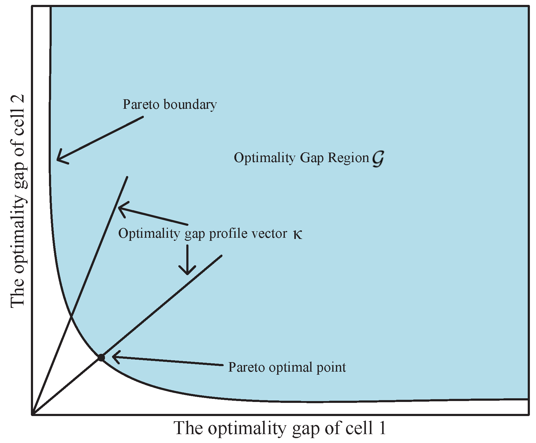
• System modeling and centralized optimization: We construct a multi-cell parallel Air-FL system model, detail the AirComp architecture between devices and APs, and establish the interference mechanisms under shared spectrum conditions. We analyze the impact of aggregation errors on the convergence of the optimality gap and formulate a power control optimization problem aimed at minimizing the total optimality gap across all cells. To characterize performance trade-offs, we employ the Pareto boundary theory and design a centralized power control algorithm to delineate the Pareto boundary.
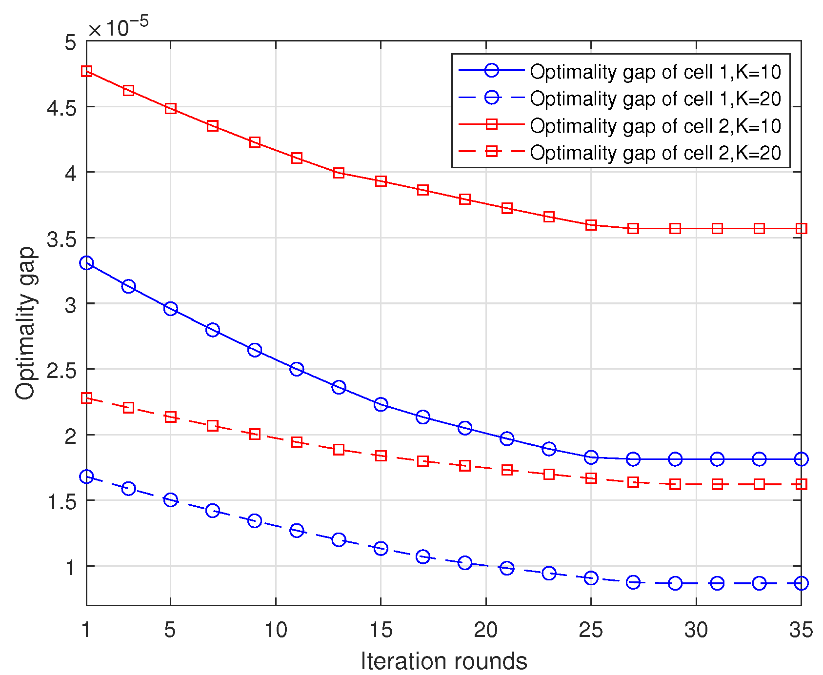
• Distributed optimization via IT: We propose a distributed optimization scheme based on IT, which decouples the globally coupled problem into locally solvable subproblems. Each cell independently adjusts its transmit power using local CSI. To address the non-convexity of the subproblems, we first transform them into convex problems and then develop an analytical solution framework grounded in Lagrangian duality theory and implement a dynamic IT update mechanism to iteratively approach the Pareto boundary.
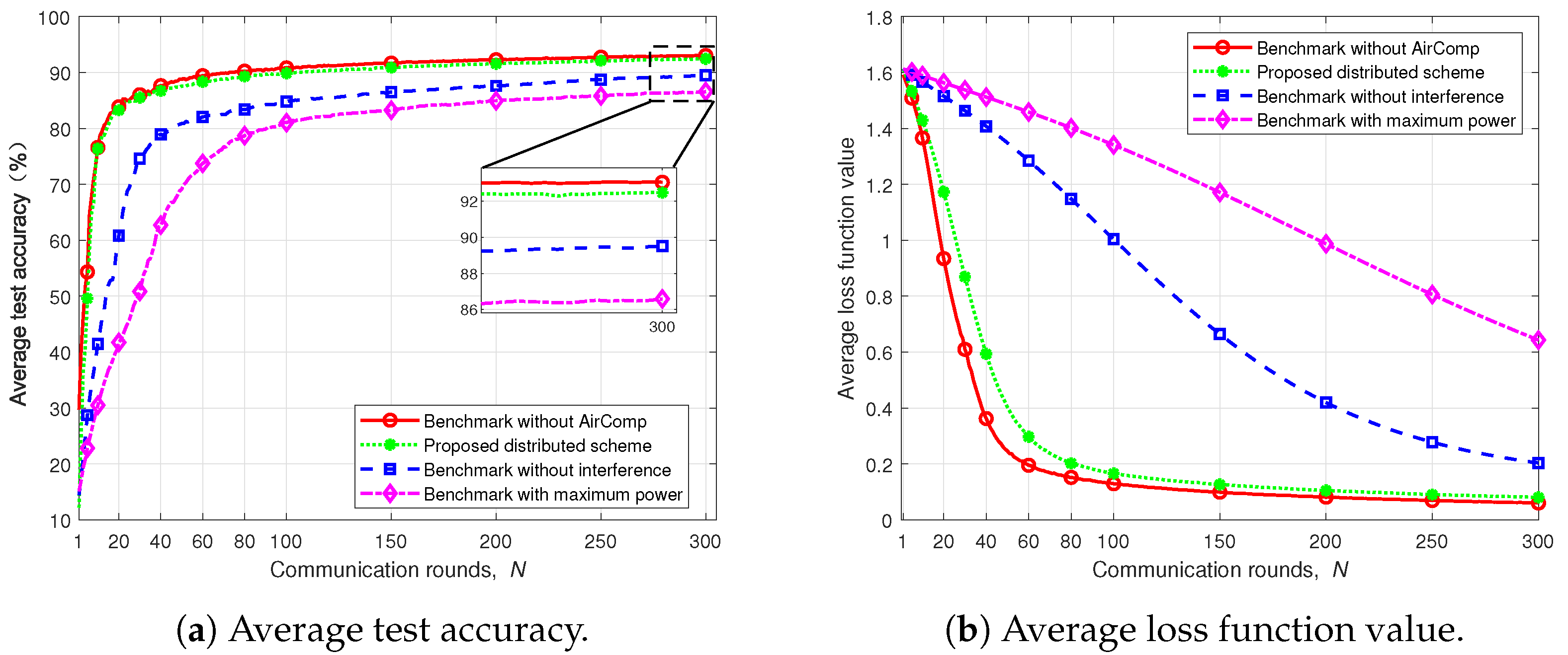
• Simulation validation: Through numerical simulations, we validate the efficacy of our proposed scheme. The results demonstrate that our approach surpasses baseline methods in terms of training convergence speed, cross-cell performance balance, and test accuracy. Moreover, it achieves stable convergence within a limited number of iterations, underscoring its practicality and effectiveness in complex multi-task edge intelligence scenarios.

The remainder of this paper is structured as follows. Section 2 introduces the parallel multi-task Air-FL system model. Section 3 examines the influence of aggregation errors on cell-level local optimality gaps, formulates a power control optimization framework, and presents the concept of the Pareto boundary. Section 4 proposes both a centralized power control optimization scheme and a distributed power control optimization scheme based on IT constraints. Section 5 provides numerical results to validate the performance of our proposed scheme. Section 6 concludes the paper.

2. System Model

As illustrated in Figure 1, we consider a parallel multi-task Air-FL system composed of M cells. Each cell includes a dedicated AP, indexed by $m\in \mathcal{M}\triangleq \{1,\dots ,M\}$, and serves K single-antenna edge devices, indexed by $k\in {\mathcal{K}}_m\triangleq \{1,\dots ,K\}$. Define the global device set as $\mathcal{K}\triangleq \{{\mathcal{K}}_1,\dots ,{\mathcal{K}}_M\}$. Each cell independently collaborates to train a distinct machine learning model, which highlights the heterogeneity across tasks.

2.1. Federated Learning Model

Each AP–device cluster forms a standalone FL system, with the m-th cell learning a cell-specific model parameterized by the vector ${\mathbf{e}}_m={[e_{m,1},\dots ,e_{m,C}]}^T$, where C is the model dimension. Each device $k\in {\mathcal{K}}_m$ holds a private local dataset ${\mathcal{D}}_k$. The sample loss function evaluates the prediction error of model parameter ${\mathbf{e}}_m$ on an input-label pair $({\mathbf{x}}_i,{\xi }_i)\in {\mathcal{D}}_k$. Accordingly, the local loss function on device k is defined as

$$\begin{array}{c}\hfill H_k\left({\mathbf{e}}_m\right)={\displaystyle \frac{1}{|{\mathcal{D}}_k|}}\sum _{({\mathbf{x}}_i,{\xi }_i)\in {\mathcal{D}}_k}{H}_k({\mathbf{e}}_m,{\mathbf{x}}_i,{\xi }_i).\end{array}$$

(1)

Assuming uniform dataset sizes within each cell, i.e., $|{\mathcal{D}}_j|=|{\mathcal{D}}_k|,\forall j,k\in {\mathcal{K}}_m$, the union of all local datasets in cell $m\in \mathcal{M}$ is denoted as ${\mathcal{D}}_m={\cup }_{k\in {\mathcal{K}}_m}{\mathcal{D}}_k$. Then, the corresponding global loss function for cell $m\in \mathcal{M}$ is expressed as

$$\begin{array}{cc}\hfill H_m\left({\mathbf{e}}_m\right)& ={\displaystyle \frac{|{\mathcal{D}}_k|}{|{\mathcal{D}}_m|}}\sum _{k\in {\mathcal{K}}_m}{H}_k\left({\mathbf{e}}_m\right)={\displaystyle \frac{1}{K}}\sum _{k\in {\mathcal{K}}_m}{H}_k\left({\mathbf{e}}_m\right).\hfill \end{array}$$

(2)

The training goal of cell $m\in \mathcal{M}$ is to find the optimal model parameter ${\mathbf{e}}_m^{★}$ that minimizes the global loss function $H_m\left({\mathbf{e}}_m\right)$, formulated as

$$\begin{array}{c}\hfill {\mathbf{e}}_m^{★}=\arg \underset{{\mathbf{e}}_m\in {\mathbb{R}}^C}{min}{H}_m\left({\mathbf{e}}_m\right).\end{array}$$

(3)

2.2. Communication Model

Each cell adopts the federated stochastic gradient descent (FedSGD) for model training, where devices compute and transmit gradients to the AP via AirComp-enabled uplink aggregation. The training is conducted over N global communication rounds, indexed by $n\in \mathcal{N}\triangleq \{1,\dots ,N\}$. At the beginning of round $n=1$, the aggregation center broadcasts a common initialization ${\mathbf{e}}^{\left(1\right)}$ to all APs, which then distribute it to their associated devices, setting their local model parameters ${\mathbf{e}}_k^{\left(1\right)}={\mathbf{e}}^{\left(1\right)},\forall k\in {\mathcal{K}}_m$. We assume that the downlink is error-free.

During each round n, device $k\in {\mathcal{K}}_m$ computes its local gradient estimate ${\mathbf{a}}_k^{\left(n\right)}$ over a randomly sampled mini-batch ${\tilde{\mathcal{D}}}_k^{\left(n\right)}\subset {\mathcal{D}}_k$, expressed as

$$\begin{array}{c}\hfill {\mathbf{a}}_k^{\left(n\right)}={\displaystyle \frac{1}{|{\tilde{\mathcal{D}}}_k^{\left(n\right)}|}}\sum _{{\mathbf{x}}_i,{\xi }_i\in {\tilde{\mathcal{D}}}_k^{\left(n\right)}}\nabla H_k({\mathbf{e}}_k^{\left(n\right)},{\mathbf{x}}_i,{\xi }_i).\end{array}$$

(4)

To align power levels and mitigate signal distortion, each device applies gradient normalization, defined as

$$\begin{array}{cc}\hfill {\overline{a}}_k^{\left(n\right)}& ={\displaystyle \frac{1}{C}}\sum _{c=1}^C{a}_{k,c}^{\left(n\right)},\hfill \end{array}$$

(5)

$$\begin{array}{cc}\hfill {\left({\upsilon }_k^{\left(n\right)}\right)}^2& ={\displaystyle \frac{1}{C}}\sum _{c=1}^C{\left(a_{k,c}^{\left(n\right)}-{\overline{a}}_k^{\left(n\right)}\right)}^2,\hfill \end{array}$$

(6)

$$\begin{array}{cc}\hfill s_{k,c}^{\left(n\right)}& ={\displaystyle \frac{a_{k,c}^{\left(n\right)}-{\overline{a}}_k^{\left(n\right)}}{{\upsilon }_k^{\left(n\right)}}},\hfill \end{array}$$

(7)

where ${\overline{a}}_k^{\left(n\right)}\in \mathbb{R}$ and ${\upsilon }_k^{\left(n\right)}\in {\mathbb{R}}_{+}$ denote the mean and standard deviation of the C dimensional local gradient ${\mathbf{a}}_k^{\left(n\right)}$, respectively. $s_{k,c}^{\left(n\right)}$ is the normalized signal to be transmitted, satisfying $\mathbb{E}\left[s_{k,c}^{\left(n\right)}\right]=0$ and $\mathbb{E}\left[{\left(s_{k,c}^{\left(n\right)}\right)}^2\right]=1$. Gradients from different devices are assumed to be statistically independent.

Each device transmits its signal over a quasi-static channel. Let $h_{m,k}^{\left(n\right)}$ denote the channel from device $k\in {\mathcal{K}}_m$ to its AP $m\in \mathcal{M}$, and $h_{m,i}^{\left(n\right)}$ denote the channel from interfering device $i\in {\mathcal{K}}_j$, $j\ne m$ to AP m. The transmission coefficient is set as $b_k^{\left(n\right)}=\sqrt{p_k^{\left(n\right)}}{\displaystyle \frac{{\left(h_{m,k}^{\left(n\right)}\right)}^H}{|h_{m,k}^{\left(n\right)}|}}$ with power $p_k^{\left(n\right)}\le P_k^{max}$, where $P_k^{max}$ is the instantaneous power budget on each device. The signal received at AP $m\in \mathcal{M}$ for the c-th model parameter is expressed as

$$\begin{array}{cc}\hfill r_{m,c}^{\left(n\right)}& =\sum _{k\in {\mathcal{K}}_m}\sqrt{p_k^{\left(n\right)}}\left|h_{m,k}^{\left(n\right)}\right|s_{k,c}^{\left(n\right)}+Z_{m,c}^{\left(n\right)}+\sum _{j\in \mathcal{M}\setminus \left\{m\right\}}\sum _{i\in {\mathcal{K}}_j}{\displaystyle \frac{\sqrt{p_i^{\left(n\right)}}{h}_{m,i}^{\left(n\right)}{\left(h_{j,i}^{\left(n\right)}\right)}^H}{|h_{j,i}^{\left(n\right)}|}}{s}_{i,c}^{\left(n\right)},\hfill \end{array}$$

(8)

where $Z_{m,c}^{\left(n\right)}\sim \mathcal{CN}(0,{\sigma }_m^2)$ denotes the additive white Gaussian noise (AWGN) with power ${\sigma }_m^2$ at the receiver of AP $m\in \mathcal{M}$.

The denoising factor ${\theta }_m^{\left(n\right)}$ is used to equalize signal power and suppress noise/interference. To reconstruct the aggregated gradient, the AP performs gradient-based linear estimation post-processing on the received signal $r_{m,c}^{\left(n\right)}$, given as

$$\begin{array}{cc}\hfill y_{m,c}^{\left(n\right)}& ={\displaystyle \frac{1}{K}}\left({\displaystyle \frac{r_{m,c}^{\left(n\right)}}{\sqrt{{\theta }_m^{\left(n\right)}}}}+\sum _{k\in {\mathcal{K}}_m}{\overline{a}}_k^{\left(n\right)}\right)\hfill \\ \hfill & ={\displaystyle \frac{1}{K}}\left(\sum _{k\in {\mathcal{K}}_m}{a}_{k,c}^{\left(n\right)}+{\displaystyle \frac{r_{m,c}^{\left(n\right)}}{\sqrt{{\theta }_m^{\left(n\right)}}}}-\sum _{k\in {\mathcal{K}}_m}\left(a_{k,c}^{\left(n\right)}-a_k^{\left(n\right)}\right)\right)\hfill \\ \hfill & =a_{m,c}^{\left(n\right)}+{\epsilon }_{m,c}^{\left(n\right)},\hfill \end{array}$$

(9)

where $a_{m,c}^{\left(n\right)}={\displaystyle \frac{1}{K}}{\sum }_{k\in {\mathcal{K}}_m}{a}_{k,c}^{\left(n\right)}$ is the desired average gradient; ${\epsilon }_{m,c}^{\left(n\right)}$ represents the aggregation error due to noise, power mismatch, and inter-cell interference, given as

$$\begin{array}{c}\hfill {\epsilon }_{m,c}^{\left(n\right)}={\displaystyle \frac{1}{K}}\left(\sum _{k\in {\mathcal{K}}_m}\left({\displaystyle \frac{\sqrt{p_k^{\left(n\right)}}\left|h_{m,k}^{\left(n\right)}\right|}{\sqrt{{\theta }_m^{\left(n\right)}}}}-{\upsilon }_k^{\left(n\right)}\right)s_{k,c}^{\left(n\right)}\right.\left.+\sum _{j\in \mathcal{M}\setminus \left\{m\right\}}\sum _{i\in {\mathcal{K}}_j}{\displaystyle \frac{\sqrt{p_i^{\left(n\right)}}{h}_{m,i}^{\left(n\right)}{\left(h_{j,i}^{\left(n\right)}\right)}^H}{\sqrt{{\theta }_m^{\left(n\right)}}\left|h_{j,i}^{\left(n\right)}\right|}}{s}_{i,c}^{\left(n\right)}+{\displaystyle \frac{Z_{m,c}^{\left(n\right)}}{\sqrt{{\theta }_m^{\left(n\right)}}}}\right).\end{array}$$

(10)

By collecting all C dimension model parameters, the average global gradient received by AP $m\in \mathcal{M}$ is given by

$$\begin{array}{c}\hfill {\widehat{\mathbf{a}}}_m^{\left(n\right)}=\Re \left\{{\mathbf{y}}_m^{\left(n\right)}\right\}=\left({\mathbf{a}}_m^{\left(n\right)}+\Re \left\{{\epsilon }_m^{\left(n\right)}\right\}\right),\end{array}$$

(11)

where ${\mathbf{a}}_m^{\left(n\right)}={[a_{m,1}^{\left(n\right)},\dots ,a_{m,c}^{\left(n\right)}]}^T,{\mathbf{y}}_m^{\left(n\right)}={[y_{m,1}^{\left(n\right)},\dots ,y_{m,c}^{\left(n\right)}]}^T,{\epsilon }_m^{\left(n\right)}={[{\epsilon }_{m,1}^{\left(n\right)},\dots ,{\epsilon }_{m,c}^{\left(n\right)}]}^T$.

Finally, the global model of cell $m\in \mathcal{M}$ is updated as

$$\begin{array}{c}\hfill {\mathbf{e}}_m^{(n+1)}={\mathbf{e}}_m^{\left(n\right)}-{\eta }_m^{\left(n\right)}{\widehat{\mathbf{a}}}_m^{\left(n\right)},\end{array}$$

(12)

where ${\eta }_m^{\left(n\right)}$ is the learning rate. This process continues until convergence or until the maximum number of communication rounds is reached.

3. Convergence Analysis and Problem Formulation

To guide the design of effective power control strategies in the proposed multi-task Air-FL system, we develop a convergence analysis framework that explicitly accounts for the impact of aggregation errors. In this framework, we adopt the optimality gap as a key performance indicator, which quantifies the deviation between the current global loss function value and the corresponding optimal value for each federated task during the n-th communication round.

3.1. Assumptions

As a preliminary step for our convergence analysis, we introduce several foundational assumptions, which are in line with those commonly utilized in prior studies [19,25,26,27,28,29]. These include the smoothness of local loss functions, bounded variance of stochastic gradients, and Polyak–Łojasiewicz condition to ensure the stability of gradient-based updates and allow the analytical derivation of learning dynamics under communication constraints.

Assumption 1

(Lipschitz Smoothness). For any cell $m\in \mathcal{M}$, the global loss function $H_m\left(\mathbf{e}\right)$ is assumed to be differentiable and $L_m$-smooth. That is, there exists a non-negative constant $L_m>0$ such that for all $\mathbf{e},\mathbf{v}\in {\mathbb{R}}^C$, the following condition holds [19,25]:

$$\begin{array}{c}\hfill ∥\nabla H_m\left(\mathbf{e}\right)-\nabla H_m\left(\mathbf{v}\right)∥\le L_m∥\mathbf{e}-\mathbf{v}∥,\end{array}$$

(13)

where $\nabla H_m\left(\mathbf{e}\right)$ denotes the gradient of the loss function. Equivalently, the following upper bound holds for the loss function:

$$\begin{array}{c}\hfill H_m\left(\mathbf{e}\right)\le H_m\left(\mathbf{v}\right)+\nabla H_m{\left(\mathbf{v}\right)}^T(\mathbf{e}-\mathbf{v})+{\displaystyle \frac{L_m}{2}}{∥\mathbf{e}-\mathbf{v}∥}^2.\end{array}$$

(14)

Assumption 2

(Bounded Variance). The local gradient estimates ${\mathbf{a}}_k^{\left(n\right)}$ are assumed to be independent and unbiased estimates of the true gradient $\nabla H_k\left({\mathbf{e}}_k\right)$ and possess bounded variance, i.e., [26,27]

$$\begin{array}{c}\hfill \mathbb{E}\left[{\mathbf{a}}_k^{\left(n\right)}\right]=\nabla H_k\left({\mathbf{e}}_k^{\left(n\right)}\right),\forall k\in \mathcal{K},\forall n\in \mathcal{N},\end{array}$$

(15)

$$\begin{array}{c}\hfill \mathbb{E}\left({∥{\mathbf{a}}_k^{\left(n\right)}-\nabla H_k\left({\mathbf{e}}_k^{\left(n\right)}\right)∥}^2\right)\le {\displaystyle \frac{{\varphi }_k^2}{n_b}},\forall k\in \mathcal{K},\forall n\in \mathcal{N},\end{array}$$

(16)

where ${\varphi }_k\ge 0$ denotes the variance of stochastic gradients at each device, and $n_b$ denotes the mini-batch size used for gradient computation. (While we assume uniform mini-batch sizes and dataset sizes across devices for analytical tractability, the stochastic gradient variance term ${\varphi }_k$ captures statistical heterogeneity arising from non-identically distributed (non-IID) local data distributions. Extensions to support heterogeneous dataset sizes and computation budgets can be incorporated by adjusting the weighting factors in the loss function and optimization problem.)

Assumption A3

(Polyak–Łojasiewicz Condition). Let $H_m^{★}$ denote the global optimal loss function value for cell m. The Polyak–Łojasiewicz condition asserts that there exists a constant ${\mu }_m\ge 0$ such that $\nabla H_m\left(\mathbf{e}\right)$ satisfies [28,29]

$$\begin{array}{c}\hfill {∥\nabla H_m\left(\mathbf{e}\right)∥}^2\ge 2{\mu }_m(H_m\left(\mathbf{e}\right)-H_m^{★}).\end{array}$$

(17)

3.2. Optimality Gap vs. Aggregation Error

Building upon the preceding assumptions, this subsection investigates the convergence behavior of parallel multi-task Air-FL, with a particular focus on how aggregation errors influence the optimality gap.

Let ${\mathbf{e}}_m^{(n+1)}$ denote the updated global model parameter for cell $m\in \mathcal{M}$ after global communication round n. The corresponding optimality gap is defined as $\mathbb{E}\left[H_m\left({\mathbf{e}}_m^{(n+1)}\right)\right]-H_m^{★}$. Let $\mathbb{E}\left[\Re {\left\{{\epsilon }_{m,c}^{\left(n\right)}\right\}}^2\right]$ represent the MSE of the global gradient estimate. With an appropriately designed diminishing learning rate, we establish the following result to characterize the convergence bound for each task.

Theorem 1.

Consider a parallel multi-task Air-FL setup where each cell $m\in \mathcal{M}$ adopts a diminishing learning rate of the form $0\le {\eta }_m^{\left(n\right)}={\displaystyle \frac{u_m}{n+v_m}}\le {\displaystyle \frac{1}{L_m}}\le {\displaystyle \frac{1}{{\mu }_m}},\forall n\in \mathcal{N}$ with constants $v_m>0,u_m>{\displaystyle \frac{1}{{\mu }_m}}$. Suppose that each device employs a fixed mini-batch size $n_b=N$. Under these settings, the expected optimality gap for each cell $m\in \mathcal{M}$ after N communication rounds is bounded by

$$\begin{array}{cc}\hfill \mathbb{E}\left[H_m\left({\mathbf{e}}_m^{(N+1)}\right)\right]-H_m^{★}\le \prod _{n\in \mathcal{N}}{D}_m^{\left(n\right)}\left(\mathbb{E}\left[H_m({\mathbf{e}}_m^1)\right]-H_m^{★}\right)& \hfill \\ \hfill +\sum _{n\in \mathcal{N}}{J}_m^{\left(n\right)}({\eta }_m^{\left(n\right)}{B}_m+L_m{({\eta }_m^{(n)})}^2\sum _{c=1}^C\mathbb{E}[\Re {\{{\epsilon }_{m,c}^{(n)}\}}^2])& ,\hfill \end{array}$$

(18)

where $D_m^{\left(n\right)}\triangleq 1-{\mu }_m{\eta }_m^{\left(n\right)}$ satisfies $0<D_m^{\left(n\right)}<1,\forall n\in \mathcal{N}$, $J_m^{\left(n\right)}\triangleq {\displaystyle \frac{{\displaystyle \prod _{i=n}^N}{D}_m^{\left(i\right)}}{2D_m^{\left(n\right)}}}$, and the gradient variance is defined as $B_m\triangleq {\displaystyle \frac{1}{K}}\sum _{k\in {\mathcal{K}}_m}{\displaystyle \frac{{\varphi }_k^2}{N}}$.

Remark 1.

The proof of Theorem 1 is similar to reference [19]. Please refer to reference [19] for more details. The convergence upper bound of the optimality gap in Theorem 1 consists of three distinct components. The first component is the initial optimality gap $D_m^{\left(n\right)}\mathbb{E}\left[H_m\left({\mathbf{e}}_m^1\right)\right]-H_m^{★}$, determined by the discrepancy between the initial point of the global loss function and its optimal value in cell $m\in \mathcal{M}$. The second component is the gradient variance term $J_m^{\left(n\right)}{\eta }_m^{\left(n\right)}{B}_m$, capturing the influence of stochastic gradient noise arising from statistical heterogeneity within the local datasets of cell m. The third component is the aggregation error term $J_m^{\left(n\right)}{L}_m{({\eta }_m^{\left(n\right)})}^2{\displaystyle \sum _{c=1}^C}\mathbb{E}\left[\Re {\{{\epsilon }_{m,c}^{\left(n\right)}\}}^2\right]$, which quantifies the cumulative effect of model aggregation errors induced by channel noise, channel fading, and inter-cell interference. In real-world deployments, the number of communication rounds is finite, and the learning rate cannot be reduced indefinitely. As a result, each cell’s optimization process converges to a neighborhood of the global minimum, characterized by a small but non-zero steady-state optimality gap.

3.3. Problem Formulation

In this subsection, building on the convergence analysis from the previous subsection, we derive the optimality gap expression and further formulate a power control optimization problem aimed at minimizing the optimality gap in each cell. From the derived upper bound, it is evident that the initial gap and gradient variance terms remain constant once the system configuration is fixed. Therefore, our attention centers on the aggregation error, which varies with the power control variables and dominates the effective optimality gap to be minimized, formulated as

$$\begin{array}{c}\hfill \sum _{n\in \mathcal{N}}\sum _{c=1}^C{J}_m^{\left(n\right)}{L}_m{({\eta }_m^{\left(n\right)})}^2\mathbb{E}\left[\Re {\{{\epsilon }_{m,c}^{\left(n\right)}\}}^2\right].\end{array}$$

(19)

To enable tractable optimization in parallel multi-task scenarios, we decouple the problem into N subproblems, each corresponding to a single communication round. Furthermore, for clarity, we focus on the aggregation error in a single dimension and omit the superscript n without loss of generality. Based on Equation (9), the MSE for the c-th model parameter in cell m is given by

$$\begin{array}{c}\hfill \mathbb{E}\left[\Re {\left\{{\epsilon }_{m,c}\right\}}^2\right]={\displaystyle \frac{1}{K^2}}\left(\sum _{k\in {\mathcal{K}}_m}{\left({\displaystyle \frac{\sqrt{p_k}\left|h_{m,k}\right|}{\sqrt{{\theta }_m}}}-{\upsilon }_k\right)}^2+\sum _{j\in \mathcal{M}\setminus \left\{m\right\}}\sum _{i\in {\mathcal{K}}_j}{\displaystyle \frac{p_i\Re {\{h_{m,i}{(h_{j,i})}^H\}}^2}{{\theta }_m|h_{j,i}{|}^2}}+{\displaystyle \frac{{\sigma }_m^2}{2{\theta }_m}}\right).\end{array}$$

(20)

Substituting this expression into (19), we obtain the following formulation for the effective optimality gap as a function of the power control variables, written as

$$\begin{array}{cc}\hfill \mathsf{\Phi }(\left\{p_k\right\},\left\{{\theta }_m\right\})\triangleq & E_m\left(\sum _{k\in {\mathcal{K}}_m}{\left({\displaystyle \frac{\sqrt{p_k}\left|h_{m,k}\right|}{\sqrt{{\theta }_m}}}-{\upsilon }_k\right)}^2+\sum _{j\in \mathcal{M}\setminus \left\{m\right\}}\sum _{i\in {\mathcal{K}}_j}{\displaystyle \frac{p_i\Re {\left\{h_{m,i}{h}_{j,i}^H\right\}}^2}{{\theta }_m{\left|h_{j,i}\right|}^2}}+{\displaystyle \frac{{\sigma }_m^2}{2{\theta }_m}}\right),\hfill \end{array}$$

(21)

where $E_m={\displaystyle \frac{J_m{L}_m{\eta }_m^2}{K^2}}$. Based on this, the optimality gap minimization problem is formulated as

$$\begin{array}{cc}\hfill \left(\mathrm{P}0\right):& \underset{\{p_k,{\theta }_m\}}{min}\left\{\mathsf{\Phi }(\left\{p_k\right\},\left\{{\theta }_m\right\})\right\}\hfill \end{array}$$

(22)

$$\begin{array}{cc}\hfill \mathrm{s}.\mathrm{t}.& 0\le {\theta }_m,\hfill \end{array}$$

(23)

$$\begin{array}{cc}\hfill & 0\le p_k\le P_k^{max},\forall k\in {\mathcal{K}}_m,m\in \mathcal{M}.\hfill \end{array}$$

(24)

Minimizing the objective function $\mathsf{\Phi }(\left\{p_k\right\},\left\{{\theta }_m\right\})$ effectively reduces the optimality gap for each cell. However, in multi-cell wireless systems, independently optimizing each cell may inadvertently amplify inter-cell interference, thus degrading the learning performance of neighboring cells.

To address this challenge and ensure fairness across distributed tasks, it is essential to introduce a theoretical framework that captures the global trade-offs among all cells’ learning performances. To this end, the next subsection introduces the concept of the Pareto boundary to characterize the optimal trade-off set of optimality gaps among cells under shared resource constraints, thereby laying a theoretical foundation for subsequent coordinated power control strategies across cells.

3.4. Pareto Boundary Definition and Characterization

To achieve balanced learning performance across different cells, we introduce the concept of the optimality gap region, denoted by $\mathcal{G}$. This region represents the set of all achievable tuples $({\mathsf{\Delta }}_1,{\mathsf{\Delta }}_2,\dots ,{\mathsf{\Delta }}_M)$, where each component ${\mathsf{\Delta }}_m$ corresponds to the optimality gap of cell $m\in \mathcal{M}$ under the given system constraints such as per-device power budgets. Formally, the optimality gap region is defined as

$$\begin{array}{c}\hfill \mathcal{G}=\bigcup \left\{\left({\mathsf{\Delta }}_1,{\mathsf{\Delta }}_2,\dots ,{\mathsf{\Delta }}_M\right)\mid {\mathsf{\Delta }}_m\ge {\mathrm{Gap}}_m,\forall m\in \mathcal{M}\right\},\end{array}$$

(25)

where ${\mathrm{Gap}}_m\triangleq J_m{L}_m{\eta }_m^2\mathbb{E}\left[\Re {\left\{{\epsilon }_{m,c}\right\}}^2\right]$ represents the minimal achievable optimality gap for cell m.

The Pareto boundary of region $\mathcal{G}$ is defined as the set of all Pareto optimal points, for which it is impossible to reduce any component ${\mathsf{\Delta }}_m$ without increasing at least one of the others. These points characterize the optimal trade-offs between the learning performance results of different cells under shared resource constraints and provide a theoretical limit to how well system-wide performance can be balanced.

To mathematically characterize the Pareto boundary, we adopt the rate profile method proposed in [30]. This method enables joint optimization across all APs by formulating a scalarized minimization problem, where the individual performance weights are specified by a profile vector $\kappa =\left[{\kappa }_1,{\kappa }_2,\dots ,{\kappa }_M\right]$. Each weight ${\kappa }_m$ reflects the relative importance or performance share assigned to cell m, subject to the normalization constraint ${\sum }_{m\in \mathcal{M}}{\kappa }_m=1$.

The optimization problem for characterizing the Pareto boundary is then given by

$$\begin{array}{cc}\hfill \left(\mathrm{P}1\right):& \underset{\{p_k,0<{\theta }_m,0<\varsigma \}}{min}\varsigma \hfill \end{array}$$

(26)

$$\begin{array}{cc}\hfill \mathrm{s}.\mathrm{t}.& {\mathrm{Gap}}_m\le {\kappa }_m\varsigma ,\forall m\in \mathcal{M},\hfill \end{array}$$

(27)

$$\begin{array}{cc}\hfill & 0\le p_k\le P_k^{max},\forall k\in {\mathcal{K}}_m,m\in \mathcal{M},\hfill \end{array}$$

(28)

where $\varsigma$ serves as an upper bound that balances the individual optimality gaps according to the profile vector $\kappa$.

For a given profile vector $\kappa$, the solution ${\varsigma }^{*}$ to problem $\left(\mathrm{P}1\right)$ determines a Pareto optimal tuple as $\kappa {\varsigma }^{*}$. Geometrically, this point lies on the intersection between the ray defined by direction $\kappa$ and the Pareto boundary of region $\mathcal{G}$. By varying $\kappa$ over the unit simplex, the entire Pareto boundary can be traced as illustrated in Figure 2, thereby fully revealing the trade-off structure among competing tasks.

4. Proposed Method

Building upon the previous section, this section develops efficient power control algorithms for parallel multi-task Air-FL from both centralized and distributed perspectives. We begin with a centralized approach that leverages full global CSI to iteratively transform and solve the non-convex optimization problem through convex reformulations. This approach enables accurate characterization of the Pareto boundary via joint optimization across all cells. However, due to the high overhead and poor scalability of centralized solutions in large-scale systems, we then propose a distributed power control scheme based on IT. The distributed approach uses only local CSI and IT constraints, and achieves near-Pareto optimal performance through inter-cell coordination without requiring a global controller.

4.1. Centralized Scheme

The main challenge in solving problem $\left(\mathrm{P}1\right)$ lies in the coupling between the transmit power $p_k$ of devices and the denoising factor ${\theta }_m$ within the expression of the optimality gap ${\mathrm{Gap}}_m$, which renders the original problem non-convex. To address this, we propose an iterative centralized algorithm. Specifically, we first fix the transmit powers $p_k$ and optimize the denoising factor ${\theta }_m$ for each cell, then substitute the resulting ${\theta }_m$ back into the original problem to solve for the optimal transmit powers. This alternating optimization (AO) continues until convergence.

4.1.1. Denoising Factor Optimization

Under fixed device transmit power, problem $\left(\mathrm{P}1\right)$ is decomposed into M independent subproblems, each corresponding to one cell, expressed as

$$\begin{array}{cc}\hfill \left(\mathrm{P}2\right):& \underset{\{0<{\theta }_m\}}{min}\left\{\sum _{k\in {\mathcal{K}}_m}{\left({\displaystyle \frac{\sqrt{p_k}\left|h_{m,k}\right|}{\sqrt{{\theta }_m}}}-{\upsilon }_k\right)}^2+\sum _{j\in \mathcal{M}\setminus \left\{m\right\}}\sum _{i\in {\mathcal{K}}_j}{\displaystyle \frac{p_i\Re {\{h_{m,i}{\left(h_{j,i}\right)}^H\}}^2}{{\theta }_m|h_{j,i}{|}^2}}+{\displaystyle \frac{{\sigma }_m^2}{2{\theta }_m}}\right\}.\hfill \end{array}$$

(29)

By introducing auxiliary variables ${\gamma }_m=1/\sqrt{{\theta }_m}$, the aforementioned problem can be reformulated into a quadratic equation, thereby enabling the straightforward derivation of the closed-form solution for the denoising factor, given as

$$\begin{array}{cc}\hfill & {\theta }_m={\left({\displaystyle \frac{\sum _{k\in {\mathcal{K}}_m}{p}_k|h_{m,k}{|}^2+{\displaystyle \sum _{j\in \mathcal{M}\setminus \left\{m\right\}}}{\displaystyle \sum _{i\in {\mathcal{K}}_j}}\frac{p_i\Re {\left\{h_{m,i}{\left(h_{j,i}\right)}^H\right\}}^2}{|h_{j,i}{|}^2}+\frac{{\sigma }_m^2}{2}}{{\displaystyle \sum _{k\in {\mathcal{K}}_m}}\sqrt{p_k}\left|h_{m,k}\right|{\upsilon }_k}}\right)}^2.\hfill \end{array}$$

(30)

4.1.2. Device Transmit Power Optimization

Substituting the solution for ${\theta }_m$ in Equation (30) back into problem $\left(\mathrm{P}1\right)$, problem $\left(\mathrm{P}1\right)$ is rewritten as

$$\begin{array}{cc}\hfill \left(\mathrm{P}3\right):& \underset{\{p_k,0<\varsigma \}}{min}\varsigma \hfill \\ \hfill \mathrm{s}.\mathrm{t}.& \left(\sum _{k\in {\mathcal{K}}_m}{\upsilon }_k^2-{\displaystyle \frac{{\kappa }_m\varsigma }{E_m}}\right)\left(\sum _{k\in {\mathcal{K}}_m}{p}_k|h_{m,k}{|}^2+\sum _{j\in \mathcal{M}\setminus \left\{m\right\}}\sum _{i\in {\mathcal{K}}_j}{\displaystyle \frac{p_i\Re {\{h_{m,i}{(h_{j,i})}^H\}}^2}{|h_{j,i}{|}^2}}+{\displaystyle \frac{{\sigma }_m^2}{2}}\right)\hfill \end{array}$$

(31)

$$\begin{array}{cc}\hfill & \le {\left(\sum _{k\in {\mathcal{K}}_m}\sqrt{p_k}\left|h_{m,k}\right|{\upsilon }_k\right)}^2,\forall m\in \mathcal{M},\hfill \end{array}$$

(32)

$$\begin{array}{cc}\hfill & 0\le p_k\le P_k^{max},\forall k\in {\mathcal{K}}_m,m\in \mathcal{M}.\hfill \end{array}$$

(33)

For any given $\varsigma$, problem $\left(\mathrm{P}3\right)$ can be reformulated as

$$\begin{array}{cc}\hfill \left(\mathrm{P}4\right):& \mathrm{Find}\left\{p_k\right\}\hfill \\ \hfill \mathrm{s}.\mathrm{t}.& {\psi }_m\left(\sum _{k\in {\mathcal{K}}_m}{p}_k|h_{m,k}{|}^2+\sum _{j\in \mathcal{M}\setminus \left\{m\right\}}\sum _{i\in {\mathcal{K}}_j}{\displaystyle \frac{p_i\Re {\{h_{m,i}{(h_{j,i})}^H\}}^2}{|h_{j,i}{|}^2}}+{\displaystyle \frac{{\sigma }_m^2}{2}}\right)\hfill \end{array}$$

(34)

$$\begin{array}{cc}\hfill & \le {\left(\sum _{k\in {\mathcal{K}}_m}\sqrt{p_k}\left|h_{m,k}\right|{\upsilon }_k\right)}^2,\forall m\in \mathcal{M},\hfill \end{array}$$

(35)

$$\begin{array}{cc}\hfill & 0\le p_k\le P_k^{max},\forall k\in {\mathcal{K}}_m,m\in \mathcal{M},\hfill \end{array}$$

(36)

where ${\psi }_m={\displaystyle \sum _{k\in {\mathcal{K}}_m}}{\upsilon }_k^2-{\displaystyle \frac{{\kappa }_m\varsigma }{E_m}}$. Introduce the interference matrix ${\mathsf{\Lambda }}_m\triangleq [{\mathsf{\Lambda }}_{m,1},{\mathsf{\Lambda }}_{m,2},\dots ,{\mathsf{\Lambda }}_{m,K_{\mathrm{tot}}}]$ with $K_{\mathrm{tot}}=KM$, defined as

$$\begin{array}{c}\hfill {\mathsf{\Lambda }}_{m,k}=\left\{\begin{array}{cc}|h_{m,k}|,\hfill & k\in {\mathcal{K}}_m,\hfill \\ {\displaystyle \frac{\Re \{h_{m,j}{\left(h_{j,i}\right)}^H\}}{|h_{j,i}|}},\hfill & k\in {\mathcal{K}}_j,j\in \mathcal{M}\setminus \left\{m\right\}.\hfill \end{array}\right.\end{array}$$

(37)

Constraint (35) can be equivalently expressed as

$$\begin{array}{c}\hfill \sqrt{{\psi }_m\left(\sum _{m\in \mathcal{M}}\sum _{k\in {\mathcal{K}}_m}{\mathsf{\Lambda }}_{m,k}^2{p}_k+{\displaystyle \frac{{\sigma }_m^2}{2}}\right)}\le \sum _{k\in {\mathcal{K}}_m}\sqrt{p_k}\left|h_{m,k}\right|{\upsilon }_k.\end{array}$$

(38)

Define $\mathbf{q}={\left[\sqrt{p_1},\sqrt{p_2},\dots ,\sqrt{p_{K_{\mathrm{tot}}}}\right]}^T$, ${\alpha }_m=\mathrm{diag}\left(\left[{\sigma }_m^2/2,{\mathsf{\Lambda }}_m\right]\right)$, ${\beta }_m={\left[{\beta }_{m,1},{\beta }_{m,2},\dots ,{\beta }_{m,K_{\mathrm{tot}}}\right]}^T$ with ${\beta }_{m,k}$ satisfying:

$$\begin{array}{c}\hfill {\beta }_{m,k}=\left\{\begin{array}{cc}|h_{m,k}|{\upsilon }_k,\hfill & k\in K_m,\hfill \\ 0,\hfill & k\in K_j,j\in \mathcal{M}\setminus \left\{m\right\}.\hfill \end{array}\right.\end{array}$$

(39)

Therefore, problem $\left(\mathrm{P}4\right)$ can be transformed into a standard second-order cone program (SOCP) problem, given as

$$\begin{array}{cc}\hfill \left(\mathrm{P}5\right):\mathrm{Find}& \left\{\mathbf{q}\right\}\hfill \end{array}$$

(40)

$$\begin{array}{cc}\hfill \mathrm{s}.\mathrm{t}.& \sqrt{{\psi }_m}∥{[1;\mathit{q}]}^T{\alpha }_m∥\le {\mathit{q}}^T{\mathit{\beta }}_m,\forall m\in \mathcal{M},\hfill \end{array}$$

(41)

$$\begin{array}{cc}\hfill & 0\le q_k\le \sqrt{P_k^{max}},\forall k\in {\mathcal{K}}_m,m\in \mathcal{M}.\hfill \end{array}$$

(42)

Problem $\left(\mathrm{P}5\right)$ can be efficiently solved using standard convex optimization solvers (e.g., CVX [31]). Once the optimal solution ${\mathbf{q}}^{*}$ is obtained, the transmit powers follow as $p_k^{*}={\left(q_k^{*}\right)}^2$. To determine the optimal ${\varsigma }^{*}$, we employ a bisection search over feasible $\varsigma$ values and solve the corresponding SOCP at each step. The complete process is summarized in Algorithm 1.

Algorithm 1: Centralized scheme for solving problem $\left(\mathrm{P}1\right)$.

1: Input: Local gradient variance ${\upsilon }_k$, profile vector $\kappa$, convergence threshold $\iota$, and maximum power budget $P_k^{max}$. 2: Set ${\varsigma }^{\mathrm{low}}\leftarrow 0$, ${\varsigma }^{\mathrm{up}}\leftarrow {min}_{m\in \mathcal{M}}\left(E_m{\sum }_{k\in {\mathcal{K}}_m}{\upsilon }_k^2/\phantom{E_m{\sum }_{k\in {\mathcal{K}}_m}{\upsilon }_k^2{\kappa }_m}{\kappa }_m\right)$. 3: while  $\left|{\varsigma }^{\mathrm{up}}-{\varsigma }^{\mathrm{low}}\right|<\iota$  do 4:    $\varsigma \leftarrow {\displaystyle \frac{{\varsigma }^{\mathrm{low}}+{\varsigma }^{\mathrm{up}}}{2}}$. 5:    Solve problem $\left(\mathrm{P}5\right)$ to obtain $p_k^{*}$. 6:    if problem $\left(\mathrm{P}5\right)$ is feasible then 7:       ${\varsigma }^{\mathrm{up}}\leftarrow \varsigma$. 8:    else 9:       ${\varsigma }^{\mathrm{low}}\leftarrow \varsigma$. 10:    end if 11: end while 12: Obtain ${\theta }_m^{*}$ based on (30). 13: Output: Optimal solutions $\{p_k^{*},{\theta }_m^{*},{\varsigma }^{*}\}$.

While the centralized scheme achieves globally optimal solutions under full CSI, it requires an aggregation center to collect information from all APs, including intra- and inter-cell channels. This introduces significant signaling overhead and limits the system’s scalability in real-world implementations. To address this, the next subsection proposes a distributed power control algorithm based on IT. In this framework, each AP requires only local CSI and interference thresholds, thereby enabling decentralized optimization while still approximating the global Pareto boundary through iterative coordination.

4.2. Distributed Scheme

This subsection investigates the decentralized power control strategy for parallel multi-task systems under IT constraints to characterize the optimality gap and the Pareto boundary.

We define ${\mathsf{\Gamma }}_{j,m}$ as the IT value representing the maximum allowable interference power from devices in cell m to AP j. This constraint ensures that the interference from cell m does not exceed a tolerable threshold at AP j, thereby enabling independent local optimization while maintaining global coordination.

Let $\mathsf{\Gamma }$ be a vector of size $M(M-1)\times 1$ containing all ${\mathsf{\Gamma }}_{j,m}$, and ${\mathsf{\Gamma }}_m$ be a vector of size $2(M-1)\times 1$ containing both ${\mathsf{\Gamma }}_{j,m}$ and ${\mathsf{\Gamma }}_{m,j}$. For AP $m\in \mathcal{M}$, replace the interference term ${\displaystyle \sum _{i\in {\mathcal{K}}_j}}{\displaystyle \frac{p_i\Re {\{h_{m,i}{(h_{j,i})}^H\}}^2}{|h_{j,i}{|}^2}}$ with ${\mathsf{\Gamma }}_{m,j}$. Define the interference channel from device $k,\forall k\in {\mathcal{K}}_m$ to neighboring cells as ${\left|g_{j,k}\right|}^2={\displaystyle \frac{\Re {\{h_{j,k}{(h_{m,k})}^H\}}^2}{|h_{m,k}{|}^2}}$. Consequently, the optimality gap minimization problem can be independently addressed at AP $m\in \mathcal{M}$, formulated as

$$\begin{array}{cc}\hfill (\mathrm{P}6.m):& \underset{\{p_k,{\theta }_m\ge 0\}}{min}{E}_{\mathrm{m}}\left(\sum _{k\in {\mathcal{K}}_m}{\left({\displaystyle \frac{\sqrt{p_k}\left|h_{m,k}\right|}{\sqrt{{\theta }_m}}}-{\upsilon }_k\right)}^2+\sum _{j\in \mathcal{M}\setminus \left\{m\right\}}{\displaystyle \frac{{\mathsf{\Gamma }}_{m,j}}{{\theta }_m}}+{\displaystyle \frac{{\sigma }_m^2}{2{\theta }_m}}\right)\hfill \end{array}$$

(43)

$$\begin{array}{cc}\hfill \mathrm{s}.\mathrm{t}.& \sum _{k\in {\mathcal{K}}_m}{p}_k|g_{j,k}{|}^2\le {\mathsf{\Gamma }}_{j,m},j\in \mathcal{M}\setminus \left\{m\right\},\hfill \end{array}$$

(44)

$$\begin{array}{cc}\hfill & 0\le p_k\le P_k^{max},\forall k\in {\mathcal{K}}_m,m\in \mathcal{M}.\hfill \end{array}$$

(45)

Due to the complex coupling relationship between the transmit power variables $p_k$ and the denoising factor ${\theta }_m$ in the objective function of problem $(\mathrm{P}6.m)$, the problem exhibits a non-convex structure and is challenging to solve. To address this, we introduce the inverse denoising factor ${\gamma }_m=1/{\theta }_m$ and an auxiliary variable $Q_k=\sqrt{p_k{\gamma }_m}$, thereby transforming problem $(\mathrm{P}6.m)$ as

$$\begin{array}{cc}\hfill \left(\mathrm{P}7\right):& \underset{\{Q_k,{\gamma }_m\ge 0\}}{min}{E}_m\left(\sum _{k\in {\mathcal{K}}_m}{\left(Q_k\left|h_{m,k}\right|-{\upsilon }_k\right)}^2+{\gamma }_m\left(\sum _{j\in \mathcal{M}\setminus \left\{m\right\}}{\mathsf{\Gamma }}_{m,j}+{\displaystyle \frac{{\sigma }_m^2}{2}}\right)\right)\hfill \end{array}$$

(46)

$$\begin{array}{cc}\hfill \mathrm{s}.\mathrm{t}.& \sum _{k\in {\mathcal{K}}_m}|Q_k{g}_{j,k}{|}^2\le {\mathsf{\Gamma }}_{j,m}{\gamma }_m,j\in \mathcal{M}\setminus \left\{m\right\},\hfill \end{array}$$

(47)

$$\begin{array}{cc}\hfill & Q_k^2\le P_k^{max}{\gamma }_m,\forall k\in {\mathcal{K}}_m,m\in \mathcal{M}.\hfill \end{array}$$

(48)

Since problem $\left(\mathrm{P}7\right)$ is a standard convex optimization problem, it can be directly solved using common convex optimization tools (e.g., CVX [31]). To further derive a closed-form expression and enhance theoretical understanding of the problem structure, we employ the Lagrangian dual method for analysis.

Let ${\left\{{\lambda }_{j,m}\right\}}_{j\in \mathcal{M}\setminus \left\{m\right\}}\ge 0$ represent the Lagrange multipliers corresponding to the j-th IT constraint, and ${\phi }_k$ denote the Lagrange multiplier associated with the k-th edge device’s power constraint. Thus, the partial Lagrangian function for AP $m\in \mathcal{M}$ is expressed as

$$\begin{array}{cc}\hfill {\mathcal{L}}_m\left(Q_k,{\gamma }_m,{\left\{{\lambda }_{j,m}\right\}}_{j\in \mathcal{M}\setminus \left\{m\right\}},{\phi }_k\right)& =E_{\mathrm{m}}\left({\sum _{k\in {\mathcal{K}}_m}\left(Q_k\left|h_{m,k}\right|-{\upsilon }_k\right)}^2\right.\hfill \\ \hfill & \left.+{\gamma }_m\left(\sum _{j\in \mathcal{M}\setminus \left\{m\right\}}{\mathsf{\Gamma }}_{m,j}+{\displaystyle \frac{{\sigma }_m^2}{2}}\right)\right)+\sum _{k\in {\mathcal{K}}_m}{\phi }_k\left(Q_k^2-P_k^{max}{\gamma }_m\right)\hfill \\ \hfill & +\sum _{j\in \mathcal{M}\setminus \left\{m\right\}}{\lambda }_{j,m}\left(\sum _{k\in {\mathcal{K}}_m}{\left|Q_k{g}_{j,k}\right|}^2-{\mathsf{\Gamma }}_{j,m}{\gamma }_m\right).\hfill \end{array}$$

(49)

This leads to the dual function

$$\begin{array}{cc}\hfill {\mathcal{R}}_m\left({\left\{{\lambda }_{j,m}\right\}}_{j\in \mathcal{M}\setminus \left\{m\right\}}\right)=& \underset{\left\{Q_k\ge 0,{\gamma }_m\ge 0\right\}}{\min }{\mathcal{L}}_m\left(Q_k,{\gamma }_m,{\left\{{\lambda }_{j,m}\right\}}_{j\in \mathcal{M}\setminus \left\{m\right\}},{\phi }_k\right)\hfill \end{array}$$

(50)

$$\begin{array}{cc}\hfill \mathrm{s}.\mathrm{t}.& Q_k^2\le P_k^{max}{\gamma }_m,\forall k\in {\mathcal{K}}_m.\hfill \end{array}$$

(51)

Therefore, the dual problem is formulated as

$$\begin{array}{c}\hfill \left(\mathrm{P}8\right):\underset{\left\{{\lambda }_{j,m}\ge 0,{\phi }_k>0\right\}}{max}{\mathcal{R}}_m\left({\left\{{\lambda }_{j,m}\right\}}_{j\in \mathcal{M}\setminus \left\{m\right\}},{\phi }_k\right).\end{array}$$

(52)

Since problem $\left(\mathrm{P}7\right)$ satisfies Slater’s condition, strong duality holds between its dual problem and the primal problem, which allows us to apply the Karush–Kuhn–Tucker (KKT) optimality conditions [32] to solve the problem. Define the optimal solutions of the dual problem as ${\left\{{\lambda }_{j,m}^{*}\right\}}_{j\in \mathcal{M}\setminus \left\{m\right\}}$ and ${\phi }_k^{*}$. According to the KKT optimality conditions, the variables $\left\{Q_k^{*},{\gamma }_m^{*},{\left\{{\lambda }_{j,m}^{*}\right\}}_{j\in \mathcal{M}\setminus \left\{m\right\}},{\phi }_k^{*}\right\}$ satisfy the following complementary slackness conditions, given as

$$\begin{array}{cc}\hfill & {\lambda }_{j,m}^{*}\ge 0,\forall j\in \mathcal{M}\setminus \left\{m\right\},{\phi }_k^{*}\ge 0,\forall k\in K_m,\hfill \end{array}$$

(53)

$$\begin{array}{cc}\hfill & {\lambda }_{j,m}\left(\sum _{k\in {\mathcal{K}}_m}|Q_k^{*}{g}_{j,k}{|}^2-{\mathsf{\Gamma }}_{j,m}{\gamma }_m^{*}\right)=0,\forall j\in \mathcal{M}\setminus \left\{m\right\},\hfill \end{array}$$

(54)

$$\begin{array}{cc}\hfill & {\phi }_k^{*}\left({\left(Q_k^{*}\right)}^2-P_k^{max}{\gamma }_m^{*}\right)=0,\forall k\in K_m,\hfill \end{array}$$

(55)

$$\begin{array}{cc}\hfill & {\nabla }_{Q_k}{\mathcal{L}}_m\left(Q_k,{\gamma }_m^{*},{\left\{{\lambda }_{j,m}^{*}\right\}}_{j\in \mathcal{M}\setminus \left\{m\right\}},{\phi }_k^{*}\right){|}_{Q_k=Q_k^{*}}=0,\hfill \end{array}$$

(56)

$$\begin{array}{cc}\hfill & {\nabla }_{{\gamma }_m}{\mathcal{L}}_m\left(Q_k^{*},{\gamma }_m,{\left\{{\lambda }_{j,m}^{*}\right\}}_{j\in \mathcal{M}\setminus \left\{m\right\}},{\phi }_k^{*}\right){|}_{{\gamma }_m={\gamma }_m^{*}}=0.\hfill \end{array}$$

(57)

To determine the optimal auxiliary variable $Q_k$ of each device, we begin by decomposing the Lagrangian dual function into $K_m$ independent subproblems, each corresponding to a device’s power optimization task. This decomposition allows for parallel optimization across devices.

The complementary slackness conditions indicate that when ${\phi }_k^{*}>0$, the power constraint is strictly tight, and the device transmits at its maximum power $P_k^{max}$. Conversely, if ${\phi }_k^{*}=0$, the device transmit power satisfies $Q_k^2\le P_k^{max}{\gamma }_m$. Accordingly, each subproblem is equivalently formulated as

$$\begin{array}{cc}\hfill \left(\mathrm{P}9\right):& \underset{\{0\le Q_k\}}{min}{E}_m{\left(Q_k\left|h_{m,k}\right|-{\upsilon }_k\right)}^2+\sum _{j\in \mathcal{M}\setminus \left\{m\right\}}{\lambda }_{j,m}|Q_k{g}_{j,k}{|}^2\hfill \end{array}$$

(58)

$$\begin{array}{cc}\mathrm{s}.\mathrm{t}.\hfill & Q_k^2\le P_k^{max}{\gamma }_m.\hfill \end{array}$$

(59)

Furthermore, according to the stationarity condition () for $Q_k$, we obtain

$$\begin{array}{cc}\hfill & {\nabla }_{Q_k}{\mathcal{L}}_m\left(Q_k,{\gamma }_m^{*},{\left\{{\lambda }_{j,m}^{*}\right\}}_{j\in \mathcal{M}\setminus \left\{m\right\}},{\phi }_k^{*}\right){|}_{Q_k=Q_k^{*}}\hfill \\ \hfill & =2E_m\left(|h_{m,k}{|}^2{Q}_k-\left|h_{m,k}\right|{\upsilon }_k\right)+2Q_k\sum _{j\in \mathcal{M}\setminus \left\{m\right\}}{\lambda }_{j,m}^{*}|g_{j,k}{|}^2=0.\hfill \end{array}$$

(60)

By rearranging the equations and considering the maximum device power constraint, the optimal solution for $Q_k$ is derived as

$$\begin{array}{c}\hfill Q_k^{*}=min\left({\displaystyle \frac{E_m{\upsilon }_k\left|h_{m,k}\right|}{E_m{\left|h_{m,k}\right|}^2+{\displaystyle \sum _{j\in \mathcal{M}\setminus \left\{m\right\}}}{\lambda }_{j,m}{\left|g_{j,k}\right|}^2}},\sqrt{P_k^{max}{\gamma }_m}\right).\end{array}$$

(61)

Similarly, to determine the optimal inverse denoising factor ${\gamma }_m$, we consider the following optimization problem:

$$\begin{array}{cc}\hfill \left(\mathrm{P}10\right):& \underset{\{0\le {\gamma }_m\}}{min}{E}_m{\gamma }_m\left(\sum _{j\in \mathcal{M}\setminus \left\{m\right\}}{\mathsf{\Gamma }}_{m,j}+{\displaystyle \frac{{\sigma }_m^2}{2}}\right)-\sum _{j\in \mathcal{M}\setminus \left\{m\right\}}{\lambda }_{j,m}{\mathsf{\Gamma }}_{j,m}{\gamma }_m-\sum _{k\in {\mathcal{K}}_m}{\phi }_k{P}_k^{max}{\gamma }_m.\hfill \end{array}$$

(62)

Applying the stationarity condition () with respect to ${\gamma }_m$, we can obtain

$$\begin{array}{cc}\hfill & {\nabla }_{{\gamma }_m}{\mathcal{L}}_m\left(Q_k^{*},{\gamma }_m,{\left\{{\lambda }_{j,m}^{*}\right\}}_{j\in \mathcal{M}\setminus \left\{m\right\}},{\phi }_k^{*}\right){|}_{{\gamma }_m={\gamma }_m^{*}}\hfill \\ \hfill & =E_m\left(\sum _{j\in \mathcal{M}\setminus \left\{m\right\}}{\mathsf{\Gamma }}_{m,j}+{\displaystyle \frac{{\sigma }_m^2}{2}}\right)-\sum _{j\in \mathcal{M}\setminus \left\{m\right\}}{\lambda }_{j,m}^{*}{\mathsf{\Gamma }}_{j,m}-\sum _{k\in {\mathcal{K}}_m}{\phi }_k^{*}{P}_k^{max}=0.\hfill \end{array}$$

(63)

Therefore, the optimal solution for ${\gamma }_m$ is derived as

$$\begin{array}{c}\hfill {\gamma }_m^{*}={\displaystyle \frac{E_m\left({\displaystyle \sum _{j\in \mathcal{M}\setminus \left\{m\right\}}}{\mathsf{\Gamma }}_{m,j}+\frac{{\sigma }_m^2}{2}\right)}{{\displaystyle \sum _{j\in \mathcal{M}\setminus \left\{m\right\}}}{\lambda }_{j,m}^{*}{\mathsf{\Gamma }}_{j,m}+\sum _{k\in {\mathcal{K}}_m}{\phi }_k^{*}{P}_k^{max}}}.\end{array}$$

(64)

To find the optimal dual variables ${\left\{{\lambda }_{j,m}^{*}\right\}}_{j\in \mathcal{M}\setminus \left\{m\right\}}$ and ${\phi }_k^{*}$, we can employ the ellipsoid method [33], which utilizes subgradients to iteratively refine the estimates of the dual variables. The subgradient for ${\left\{{\lambda }_{j,m}\right\}}_{j\in \mathcal{M}\setminus \left\{m\right\}}$ is ${\displaystyle \sum _{k\in {\mathcal{K}}_m}}{\left|Q_k^{*}{g}_{j,k}\right|}^2-{\mathsf{\Gamma }}_{j,m}{\gamma }_m^{*}$, and the subgradient for ${\phi }_k^{*}$ is ${\left(Q_k^{*}\right)}^2-P_k^{max}{\gamma }_m^{*}$. By iteratively updating ${\left\{{\lambda }_{j,m}\right\}}_{j\in \mathcal{M}\setminus \left\{m\right\}}$ and ${\phi }_k^{*}$ using these subgradients, the ellipsoid method converges to the optimal dual variables. Once the optimal dual variables are obtained, these variables can be substituted back into the expressions (61) and (64) to determine the optimal primal variables.

Finally, the optimal transmit power $p_k^{*}$ and the denoising factor ${\theta }_m^{*}$ are computed as

$$\begin{array}{c}\hfill p_k^{*}=min\left({\left({\displaystyle \frac{E_m{\upsilon }_k\left|h_{m,k}\right|{\theta }_m^{*}}{E_m{\left|h_{m,k}\right|}^2+{\displaystyle \sum _{j\in \mathcal{M}\setminus \left\{m\right\}}}{\lambda }_{j,m}^{*}{\left|g_{j,k}\right|}^2}}\right)}^2,P_k^{max}\right),\end{array}$$

(65)

$$\begin{array}{c}\hfill {\theta }_m^{*}={\displaystyle \frac{{\displaystyle \sum _{j\in \mathcal{M}\setminus \left\{m\right\}}}{\lambda }_{j,m}^{*}{\mathsf{\Gamma }}_{j,m}+{\displaystyle \sum _{k\in {\mathcal{K}}_m}}{\phi }_k^{*}{P}_k^{max}}{E_m\left({\displaystyle \sum _{j\in \mathcal{M}\setminus \left\{m\right\}}}{\mathsf{\Gamma }}_{m,j}+\frac{{\sigma }_m^2}{2}\right)}}.\end{array}$$

(66)

These results indicate that when ${\phi }_k^{*}>0$, the device transmits at its maximum power $P_k^{max}$. Otherwise, the transmit power is adjusted based on the regularized inverse power transmission strategy, where the regularization term ${\displaystyle \sum _{j\in \mathcal{M}\setminus \left\{m\right\}}}{\lambda }_{j,m}^{*}{\left|g_{j,k}\right|}^2$ accounts for inter-cell interference. The denoising factor ${\theta }_m^{*}$ is influenced by both inter-cell interference and the power constraints of all devices. While these solutions satisfy the inter-cell interference constraints, they are limited to scenarios with fixed interference thresholds and may not achieve Pareto optimality. Therefore, an iterative algorithm for optimizing inter-cell interference thresholds is proposed to enhance overall system performance.

To facilitate efficient distributed power control in parallel multi-task Air-FL systems, this paper introduces the concept of IT as a pivotal coordination variable to establish a local information-driven distributed optimization framework. (The proposed analysis and algorithms assume quasi-static channel conditions, where wireless links remain constant over each communication round. This assumption enables tractable optimization and reliable gradient aggregation using AirComp. In practical scenarios with mobility or fading, channel variations may affect aggregation accuracy. Nonetheless, our distributed scheme relies only on local CSI and permits iterative IT updates, offering inherent adaptability to slow channel variations. Future work may consider extending the framework to incorporate robust optimization techniques for time-varying or uncertain CSI, thereby improving resilience under mobility and fading.) Building upon this foundation, an iterative collaborative algorithm is proposed, wherein APs dynamically adjust mutual IT values through peer-to-peer signaling interactions.

In each iteration, the system selects a pair of APs for local collaborative updates. These updates are designed to ensure that the optimality gap of the local cell does not increase, nor does the performance of other cells degrade, thereby guaranteeing non-decreasing overall system performance. To implement this mechanism, it is assumed that APs possess basic backhaul link support for essential information sharing and synchronization of interference parameters.

However, determining whether the system achieves Pareto optimality under arbitrary IT configurations remains challenging. To address this, a lemma is proposed to characterize the necessary constraints between IT and the cell optimality gap under Pareto optimality conditions. This lemma provides a theoretical foundation for subsequent algorithm design.

Lemma 1

(Necessary Condition for Pareto Optimality). Under any given IT configuration Γ, if the optimality gap $\overline{{\mathsf{\Delta }}_m}\left({\mathsf{\Gamma }}_m\right)$ has reached a Pareto optimal state, then for any pair of APs m and j, the determinant of the following $2\times 2$ matrix ${\mathbf{T}}_{j,m}$ must be zero, given as [34]

$$\begin{array}{cc}\hfill {\mathbf{T}}_{j,m}& =\left[\begin{array}{cc}{\displaystyle \frac{\partial \overline{{\mathsf{\Delta }}_m}\left({\mathsf{\Gamma }}_m\right)}{\partial {\mathsf{\Gamma }}_{j,m}}}& {\displaystyle \frac{\partial \overline{{\mathsf{\Delta }}_m}\left({\mathsf{\Gamma }}_m\right)}{\partial {\mathsf{\Gamma }}_{m,j}}}\\ {\displaystyle \frac{\partial \overline{{\mathsf{\Delta }}_j}\left({\mathsf{\Gamma }}_j\right)}{\partial {\mathsf{\Gamma }}_{j,m}}}& {\displaystyle \frac{\partial \overline{{\mathsf{\Delta }}_j}\left({\mathsf{\Gamma }}_j\right)}{\partial {\mathsf{\Gamma }}_{m,j}}}\end{array}\right].\hfill \end{array}$$

(67)

Building upon the previously established analytical framework, we now delve into the derivation of the matrix elements within the IT optimization context. By solving both the primal and dual formulations of the problem, we obtain explicit expressions for each component of the matrix ${\mathbf{T}}_{j,m}$, which encapsulates the sensitivity of the optimality gaps to variations in IT parameters.

Specifically, the partial derivatives of the optimality gap $\overline{{\mathsf{\Delta }}_m}\left({\mathsf{\Gamma }}_m\right)$ with respect to the IT parameters ${\mathsf{\Gamma }}_{j,m}$ and ${\mathsf{\Gamma }}_{m,j}$ are given by

$$\begin{array}{c}\hfill {\displaystyle \frac{\partial \overline{{\mathsf{\Delta }}_m}\left({\mathsf{\Gamma }}_m\right)}{\partial {\mathsf{\Gamma }}_{j,m}}}=-{\lambda }_{j,m}^{*}{\gamma }_m^{*},{\displaystyle \frac{\partial \overline{{\mathsf{\Delta }}_j}\left({\mathsf{\Gamma }}_j\right)}{\partial {\mathsf{\Gamma }}_{m,j}}}=-{\lambda }_{m,j}^{*}{\gamma }_j^{*},\end{array}$$

(68)

where $\left\{{\lambda }_{j,m}^{*},{\lambda }_{m,j}^{*}\right\}$ respectively denote the optimal dual multipliers associated with the IT constraints in the primal problems of cell m and cell j, and $\left\{{\gamma }_m^{*},{\gamma }_j^{*}\right\}$ are the corresponding optimal inverse denoising factors.

Additionally, the derivatives with respect to the reciprocal IT parameters are written as

$$\begin{array}{c}\hfill {\displaystyle \frac{\partial \overline{{\mathsf{\Delta }}_m}\left({\mathsf{\Gamma }}_m\right)}{\partial {\mathsf{\Gamma }}_{m,j}}}=E_m{\gamma }_m^{*},{\displaystyle \frac{\partial \overline{{\mathsf{\Delta }}_j}\left({\mathsf{\Gamma }}_j\right)}{\partial {\mathsf{\Gamma }}_{j,m}}}=E_j{\gamma }_j^{*}.\end{array}$$

(69)

To iteratively refine the IT vector $\mathsf{\Gamma }$, we focus on updating only the mutual IT parameters between a selected pair of APs m and j, while keeping the rest unchanged, which is defined as

$$\begin{array}{c}\hfill {\left[{{\mathsf{\Gamma }}^{\prime }}_{j,m},{{\mathsf{\Gamma }}^{\prime }}_{m,j}\right]}^T={\left[{\mathsf{\Gamma }}_{j,m},{\mathsf{\Gamma }}_{m,j}\right]}^T+{\delta }_{j,m}·{\mathit{t}}_{j,m},\end{array}$$

(70)

where ${\mathsf{\Gamma }}^{\prime }$ represents the updated IT vector; ${\delta }_{j,m}$ denotes a suitably small step size; and ${\mathit{t}}_{j,m}$ is a vector ensuring that the product ${\mathit{T}}_{j,m}{\mathit{t}}_{j,m}<0$, thereby guaranteeing a reduction in the optimality gaps.

Assuming ${\mathbf{T}}_{j,m}=\left[\begin{array}{cc}a& b\\ c& d\end{array}\right]$, a feasible solution for ${\mathit{t}}_{j,m}$ is computed as

$$\begin{array}{c}\hfill {\mathit{t}}_{j,m}=\mathrm{sign}\left(bc-ad\right)·{\left[{\ell }_{j,m}d-b,a-{\ell }_{j,m}c\right]}^T,\end{array}$$

(71)

where ${\ell }_{j,m}$ is a ratio parameter that modulates the relative reduction rate of the optimality gap between APs m and j; $\mathrm{sign}\left(·\right)$ denotes the sign function.

By adjusting ${\ell }_{j,m}$, we can control the balance of improvement between the two APs. Specifically, setting ${\ell }_{j,m}\ge 1$ prioritizes AP m, while ${\ell }_{j,m}\le 1$ favors AP j. Through the careful selection of ${\delta }_{j,m}$ and ${\ell }_{j,m}$, we can navigate the Pareto boundary to identify configurations where no AP performance can be improved without degrading the others.

This iterative approach culminates in a distributed power control algorithm that leverages IT optimization to enhance overall system efficiency. The complete algorithm is encapsulated in Algorithm 2, which systematically updates the IT parameters to converge towards Pareto-optimal configurations. (The proposed distributed scheme currently assumes uniform data and computational resources across devices. In practice, edge devices may exhibit heterogeneity in dataset sizes, local data distributions, and processing capabilities. Our framework can accommodate such variations by incorporating per-device weighting or fairness constraints in the optimization objectives. Extending the algorithm to explicitly model non-IID data and device-level heterogeneity is a promising direction for future research).

The distributed algorithm outlined above incrementally minimizes the global optimality gap across all APs through iterative, pairwise updates of IT parameters. (Although our distributed power optimization framework shares a conceptual similarity with some interference-constrained optimization methods (e.g., [35]), there are key distinctions. In [35], the objective is to enhance location privacy and spectrum efficiency in cognitive radio networks through spectrum sharing policies, typically under single-task settings. In contrast, our work addresses a fundamentally different problem of minimizing the learning optimality gap in multi-task Air-FL systems. Furthermore, our framework integrates gradient aggregation distortion, Pareto boundary trade-offs, and an iterative IT update mechanism that collectively enable decentralized learning coordination, which is different from [35].) In each iteration, a selected pair of APs adjusts their mutual IT levels to reduce their respective optimality gaps. Crucially, these adjustments are designed to ensure that the optimality gaps of other APs in the network remain unaffected, thereby preserving overall system stability.

Algorithm 2: IT-based decentralized scheme for solving problem $\left(\mathrm{P}1\right)$.

1: Input: IT vector $\mathsf{\Gamma }$, convergence threshold $\iota$. 2: for any pair of APs m and j, $j\in \mathcal{M}\setminus \left\{m\right\}$ do 3:    if $\left|{\mathbf{T}}_{j,m}\right|>\iota$ then 4:       APs m and j synchronously update their current IT values via a reliable backhaul link. 5:       APs m and j solve problem $\left(\mathrm{P}7\right)$ to obtain optimal solution ${\left\{p_k^{*}\right\}}_{k\in {\mathcal{K}}_m}$, ${\left\{p_i^{*}\right\}}_{i\in {\mathcal{K}}_j}$, $\left\{{\theta }_m^{*},{\theta }_j^{*}\right\}$, $\left\{{\lambda }_{j,m}^{*},{\lambda }_{m,j}^{*}\right\}$. 6:       APs m and j update the elements in ${\mathbf{T}}_{j,m}$ based on (68) and (69) 7:       APs m and j exchange elements in ${\mathbf{T}}_{j,m}$ via the backhaul link, reconstruct ${\mathbf{T}}_{j,m}$ via (67), and compute ${\mathbf{t}}_{j,m}$ via (71). 8:       APs m and j update their IT values ${\mathsf{\Gamma }}_{j,m}^{\prime }$ according to (70). 9:    end if 10: end for 11: Output: Optimal device transmit power $p_k^{*}$ and optimal denoising factor ${\theta }_m^{*}$.

This iterative update mechanism guides the system’s performance toward the Pareto boundary of the optimality gap region. By carefully selecting step sizes and direction vectors for IT adjustments, the algorithm ensures that each update leads to a non-increasing optimality gap for the involved APs. Over successive iterations, this process converges to a state where no further reductions in optimality gaps are possible without adversely affecting other APs, which signifies Pareto optimality.

Compared to the initial configurations or schemes where each AP optimizes independently, this cooperative approach achieves a more efficient global performance. It encourages APs to participate in collaborative adjustments, even when such changes may not immediately benefit their individual performance metrics. This collaborative behavior is facilitated by the algorithm’s design, which ensures that any trade-offs made by individual APs contribute to the overall reduction in the system’s optimality gap. Such approaches highlight the potential of decentralized coordination mechanisms in enhancing the efficiency and fairness of distributed wireless systems.

5. Numerical Results

In this section, we present the simulation results to evaluate the performance of the proposed distributed scheme in multi-task Air-FL scenarios. Specifically, we consider two representative tasks: ridge regression on synthetic datasets and handwritten digit classification using the Modified National Institute of Standards and Technology (MNIST) dataset. These experiments aim to assess the effectiveness of the distributed scheme in managing interference and optimizing learning performance across multiple tasks. (While MNIST and synthetic regression tasks are used in our simulations for clarity and analytical convenience, the proposed distributed power control framework is compatible with more complex datasets and deep neural models. Our goal in this paper is to highlight the impact of interference-aware power optimization on FL performance under multi-task and multi-cell settings.)

5.1. Simulation Setup and Benchmark Schemes

We simulate a two-cell network, each hosting a distinct FL task. The first cell is centered at coordinates $(0,0)$, and the second at $(40,0)$. Devices within each cell are randomly distributed within a 20-meter radius around their respective APs. The wireless channels between devices and APs follow a distance-dependent Rayleigh fading model. (In this study, we adopt Rayleigh fading to model the wireless channels between APs and devices. This choice captures a rich-scattering, non-line-of-sight (NLoS) environment and allows for tractable performance evaluation. However, we acknowledge that practical deployments may involve line-of-sight (LoS) components, in which case Rician or Nakagami-m fading models may provide more accurate characterizations. Incorporating such models to study the impact of LoS-dominant fading on Air-FL performance is an important direction for future work.) The channel gain between device k and AP m is modeled as $h_{m,k}=\sqrt{{\mathsf{\Omega }}_0{d}_{m,k}^{-\zeta }}{h}_0$, where ${\mathsf{\Omega }}_0$ denotes the path loss at a reference distance of 1 m; $\zeta$ is the path loss exponent; $d_{m,k}$ is the distance between device k and AP m; and $h_0\sim \mathcal{C}\mathcal{N}(0,I)$ is a complex Gaussian random variable with zero mean and unit variance. Interference channels between devices and non-associated APs are modeled similarly. Simulation parameters are detailed in

Table 2. Simulation parameters.

Parameter	Value
K	10
$K_{\mathrm{tot}}$	20
${\mathsf{\Omega }}_0$	$-60$ dB
$\zeta$	3
${\sigma }_m^2$	${10}^{-7}$ W
$P_k^{max}$	1 W
$\iota$	${10}^{-9}$
${\ell }_{j,m}$	$0.5$
${\eta }_1^{\left(n\right)}$	$2/(n+8)$
${\eta }_2^{\left(n\right)}$	$2/(n+10)$

.

In terms of performance metrics, the optimality gap and prediction error are used to evaluate the ridge regression task on the synthetic dataset. To benchmark the proposed distributed scheme, we compare it against the following baseline methods:

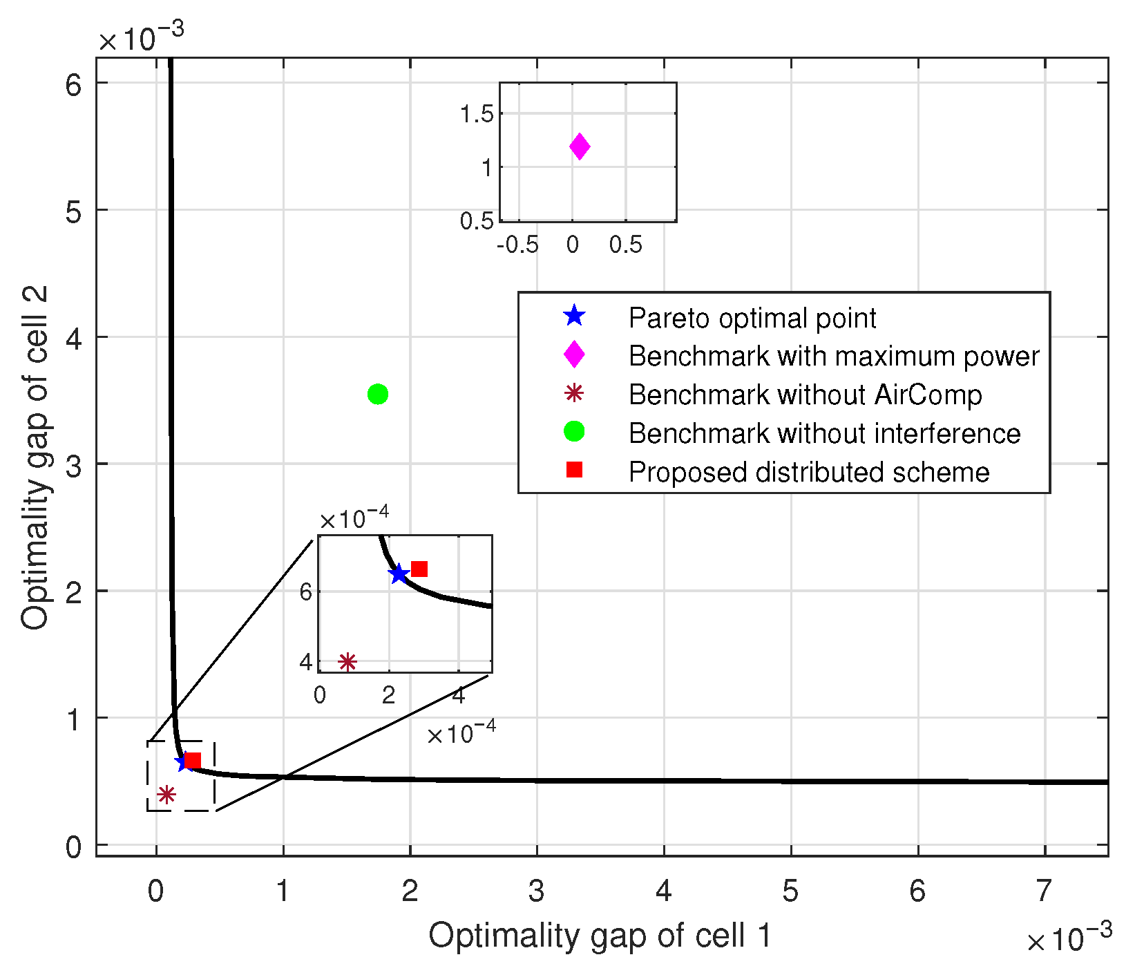
• Benchmark with maximum power: In this scheme, all devices transmit at their maximum power levels, i.e., $p_k=p_k^{max}$. This scheme requires no CSI collection and represents the simplest power control strategy.
• Benchmark without AirComp: In this scheme, all devices transmit their local model updates to their respective APs, which perform aggregation without any interference. This scenario assumes an ideal communication environment, serving as an upper performance bound.
• Benchmark without interference: In this scheme, each AP optimizes the device transmit power and denoising factor based solely on intra-cell CSI, without coordinating with other APs. The optimization problem for AP m is formulated as

  $$\begin{array}{cc}\hfill \underset{\{0\le p_k\le p_k^{max},0\le {\theta }_m\}}{min}& E_m\left(\sum _{k\in {\mathcal{K}}_m}{\left({\displaystyle \frac{\sqrt{p_k}\left|h_{m,k}\right|}{\sqrt{{\theta }_m}}}-{\upsilon }_k\right)}^2+{\displaystyle \frac{{\sigma }_m^2}{2{\theta }_m}}\right).\hfill \end{array}$$

  (72)

5.2. Multi-Task Ridge Regression Performance

We consider that each cell independently trains a ridge regression model on distinct datasets. Each cell’s dataset follows a unique distribution, which reflects heterogeneous data environments. The sample loss function for cell $m\in \mathcal{M}$ is defined as

$$\begin{array}{c}\hfill H_m({\mathbf{e}}_m,{\mathbf{x}}_m,{\tau }_m)={\displaystyle \frac{1}{2}}{∥{\mathit{x}}_m^T{\mathbf{e}}_m-{\tau }_m∥}^2+\rho R\left({\mathbf{e}}_m\right),\end{array}$$

(73)

where $\rho =5\times {10}^{-5}$ is the regularization hyperparameter. The input sample vector ${\mathbf{x}}_m\in {\mathbb{R}}^C$ for each cell is drawn from a standard normal distribution, i.e., ${\mathbf{x}}_m\sim \mathcal{N}(\mathbf{0},\mathbf{I})$, with model dimension $C=20$. The target labels for each cell are generated as ${\tau }_1=x_1\left(2\right)+3x_1\left(5\right)+0.2z$ and ${\tau }_2=x_2\left(3\right)+2x_2\left(8\right)+4x_2\left(10\right)+0.3z$, where z represents standard Gaussian noise. Each device within a cell holds $D_k=500,\forall k\in \mathcal{K}$ data samples, resulting in a total of $D_{\mathrm{m}}={\sum }_{k\in \mathcal{K}}{D}_k=5000$ samples per cell.

To evaluate the convergence behavior, we compute the smoothness parameter $L_m$ and the Polyak–Łojasiewicz parameter ${\mu }_m$ for each cell as in Assumptions A1 and A3, based on the eigenvalues of the sample covariance matrix ${\mathbf{X}}_m^T{\mathbf{X}}_m/D_m+{10}^{-4}\mathbf{I}$ [36].

The optimal model parameters ${\mathbf{e}}_m^{★}$ are obtained as ${\mathbf{e}}_m^{★}={({\mathbf{X}}_m^T{\mathbf{X}}_m+\rho \mathbf{I})}^{-1}{\mathbf{X}}_m^T{\mathbf{\tau }}_m$ with ${\mathbf{\tau }}_m={[{\tau }_1,\dots ,{\tau }_{D_m}]}^T$. The initial model for each cell is initialized as a zero vector.

Figure 3 presents the evolution of the optimality gap and prediction error across communication rounds N for various power control strategies in both cells. The proposed distributed scheme demonstrates a consistent decline in both metrics as N increases, with the prediction error stabilizing in later rounds. This trend indicates that the local models of both cells progressively converge towards their respective optimal solutions on the training set and ultimately achieve strong generalization performance on the test set. Analyzing the performance disparity between the two cells, Cell 1 consistently exhibits superior outcomes in both optimality gap and prediction error. This advantage is primarily due to the simpler label structure and lower data noise in Cell 1’s task, thereby enabling more efficient learning and faster convergence under identical training conditions. Comparative assessments reveal that the proposed distributed scheme significantly outperforms both the benchmark with maximum power and benchmark without interference in both cells. Specifically, the proposed scheme not only accelerates the reduction in training errors to bring the model closer to the optimal training solution but also enhances generalization capability as evidenced by the lower prediction errors on the test set. This performance underscores its effectiveness in balancing rapid convergence with robust generalization. Furthermore, Figure 3 also includes the benchmark without AirComp as an ideal performance upper bound. In later communication rounds, the prediction error achieved by the proposed distributed scheme closely approaches this ideal benchmark with only a marginal gap. This proximity illustrates the scheme’s capacity to approximate optimal performance despite practical challenges such as communication losses and inter-cell interference. In contrast, other baseline schemes continue to exhibit significant error at high communication rounds, particularly the benchmark with maximum power, which highlights their limitations in achieving efficient convergence and generalization.

Figure 4 illustrates the achievable regions of the optimality gap for two cells at communication rounds $N=100$. The Pareto boundary is delineated by varying the profile vector of the centralized power control scheme as $\kappa =[{\kappa }_m,1-{\kappa }_m]$, where ${\kappa }_m=\left[0.001,0.01,0.1,0.3,0.4,0.5,0.6,0.7,0.9,0.99,0.999\right]$. The bottom-leftmost point on the Pareto boundary by the centralized scheme represents the Pareto-optimal point, while the bottom-leftmost point by the benchmark without AirComp denotes the idealized learning performance, which serves as a benchmark for evaluating the proximity of practical schemes to optimal performance. It is observed that the Pareto-optimal point lies closest to this idealized benchmark, indicating that the centralized scheme achieves the best practical performance. Furthermore, the proposed distributed scheme demonstrates a performance remarkably closer to the Pareto-optimal point, with deviations within ${10}^{-4}$, which demonstrates its efficacy in approaching centralized optimality. This proximity underscores its practical applicability, especially in scenarios constrained by communication resources. In contrast, the benchmark without interference exhibits inferior overall performance, which highlights the importance of considering inter-cell dynamics. The benchmark with maximum power performs the worst due to a lack of power adjustment or interference management.

Figure 5 demonstrates the convergence behavior of the proposed distributed scheme by depicting the evolution of the optimality gap for Cell 1 and Cell 2 across iterative rounds with $K=10$ and $K=20$ devices per cell. The results demonstrate that all schemes converge within 30 rounds. (While our scheme demonstrates convergence within approximately 30 global rounds, we do not compare directly with FedAvg or FedProx, as these methods operate under fundamentally different assumptions. As such, we evaluate against baselines that are aligned with our system model to ensure a fair and meaningful comparison.) Comparative analysis between the two device configurations reveals that, under the same number of iterations, the scenario with $K=20$ devices per cell attains a significantly lower optimality gap than the $K=10$ scenario. This suggests that incorporating more devices into the optimization process enhances the overall system performance, which drives the learning outcomes closer to the optimal solution. Such scalability is crucial for practical applications, where the number of participating devices can vary. While an increased number of devices introduces greater complexity in collaborative computation and power adjustment, potentially leading to a slight reduction in convergence speed, the algorithm maintains stable convergence within a limited number of iterations. This resilience confirms the effectiveness of the proposed distributed scheme in managing complex multi-cell scenarios, thereby ensuring reliable performance even as the network scales.

5.3. Performance on Multi-Task MNIST Dataset

We establish a parallel multi-task handwritten digit classification scenario utilizing the MNIST dataset. Specifically, Cell 1 and Cell 2 are assigned distinct subsets of digit classes, labeled as 0–4 and 5–9, respectively. This configuration introduces task heterogeneity, as each cell processes non-overlapping label distributions. Both cells employ an identical convolutional neural network (CNN) architecture for local model training. The architecture comprises two convolutional layers with rectified linear unit (ReLU) activation functions and kernel sizes of $5\times 5$, containing 32 and 64 channels, respectively. Each convolutional layer is followed by a $2\times 2$ max-pooling operation. Subsequently, the network includes a fully connected layer with 1024 units, culminating in a softmax output layer for classification. During local training, all devices utilize a fixed mini-batch size of $m_b=128$. The performance of the models is evaluated using the average test accuracy and loss function values of both cells to provide a comprehensive assessment of classification efficacy and convergence behavior within the multi-task learning system.

Figure 6 illustrates the impact of communication rounds N on the overall performance of parallel multi-task Air-FL over the MNIST dataset. From Figure 6a, all schemes demonstrate a continuous improvement in average test accuracy as N increases, with convergence observed in the later stages. The benchmark without AirComp serves as the performance upper bound, which achieves optimal accuracy. Notably, the proposed distributed scheme closely approaches this ideal benchmark throughout the training process, with an optimal test accuracy difference within $1\%$. This proximity demonstrates its near-optimal classification performance, which surpasses both the benchmark without interference and the benchmark with maximum power, thereby validating its superior convergence speed and learning efficacy. Figure 6b reveals that the average loss function value decreases across all schemes, albeit with varying rates of decline and final convergence levels. The proposed distributed scheme achieves a loss function value closer to the optimal performance of the benchmark without AirComp compared to other baseline schemes. This outcome highlights its capability to effectively enhance the model’s generalization performance.

6. Conclusions

This paper addressed the challenge of inter-cell interference in parallel multi-task Air-FL systems, where each cell independently trains a distinct model while simultaneously performing over-the-air aggregation. We analyzed how aggregation errors impact the local optimality gap and proposed a joint optimization framework for device transmit power and denoising factors aimed at minimizing the cumulative optimality gap across all cells. To characterize the trade-offs in multi-cell performance, we employed Pareto boundary theory and designed a centralized optimization scheme that serves as a performance upper bound. Building upon this, we introduced a distributed power control strategy based on IT, which decouples the globally coupled problem into locally solvable subproblems. This approach allows each cell to independently adjust its transmit power using only local CSI. To enhance computational efficiency, we derived closed-form solutions for the subproblems through Lagrangian duality theory and implemented a dynamic IT update mechanism to effectively approach the Pareto boundary. Simulation results demonstrated that the proposed distributed scheme outperforms benchmark methods in terms of training convergence speed, cross-cell performance balance, and test accuracy. Future work will extend our framework to larger-scale and more heterogeneous datasets such as CIFAR-10, which will enable validation under non-convex learning objectives and more realistic visual data distributions. This will further demonstrate the scalability and robustness of our distributed scheme.

References

1. Verbraeken, J.; Wolting, M.; Katzy, J.; Kloppenburg, J.; Verbelen, T.; Rellermeyer, J.S. A survey on distributed machine learning. ACM Comput. Surv. 2020, 53, 1–33. [Google Scholar] [CrossRef]
2. Wang, S.; Tuor, T.; Salonidis, T.; Leung, K.K.; Makaya, C.; He, T.; Chan, K. When edge meets learning: Adaptive control for resource-constrained distributed machine learning. In Proceedings of the IEEE Conference on Computer Communications (INFOCOM), Honolulu, HI, USA, 16–19 April 2018; pp. 63–71. [Google Scholar] [CrossRef]
3. McMahan, B.; Moore, E.; Ramage, D.; Hampson, S.; Arcas, B.A. Communication-Efficient Learning of Deep Networks from Decentralized Data. arXiv 2017, arXiv:1602.05629v4. [Google Scholar]
4. Imteaj, A.; Thakker, U.; Wang, S.; Li, J.; Amini, M.H. A survey on federated learning for resource-constrained IoT devices. IEEE Internet Things J. 2022, 9, 1–24. [Google Scholar] [CrossRef]
5. Zhou, C.; Liu, J.; Jia, J.; Zhou, J.; Zhou, Y.; Dai, H.; Dou, D. Efficient device scheduling with multi-job federated learning. In Proceedings of the AAAI Conference on Artificial Intelligence, Online, 22 February–1 March 2022; pp. 9971–9979. [Google Scholar] [CrossRef]
6. Ma, H.; Guo, H.; Lau, V.K.N. Communication-efficient federated multitask learning over wireless networks. IEEE Internet Things J. 2023, 10, 609–624. [Google Scholar] [CrossRef]
7. Sami, H.U.; Güler, B. Over-the-air clustered federated learning. IEEE Trans. Wirel. Commun. 2023, 23, 7877–7893. [Google Scholar] [CrossRef]
8. Cao, X.; Başar, T.; Diggavi, S.; Eldar, Y.C.; Letaief, K.B.; Poor, H.V.; Zhang, J. Communication-efficient distributed learning: An overview. IEEE J. Sel. Areas Commun. 2023, 41, 851–873. [Google Scholar] [CrossRef]
9. Cao, X.; Lyu, Z.; Zhu, G.; Xu, J.; Xu, L.; Cui, S. An overview on over-the-air federated edge learning. IEEE Wirel. Commun. 2024, 31, 202–210. [Google Scholar] [CrossRef]
10. Wang, Z.; Zhao, Y.; Zhou, Y.; Shi, Y.; Jiang, C.; Letaief, K.B. Over-the-air computation for 6G: Foundations, technologies, and applications. IEEE Internet Things J. 2024, 11, 24634–24658. [Google Scholar] [CrossRef]
11. Şahin, A.; Yang, R. A survey on over-the-air computation. IEEE Commun. Surv. Tuts. 2023, 25, 1877–1908. [Google Scholar] [CrossRef]
12. Zhu, J.; Shi, Y.; Zhou, Y.; Jiang, C.; Chen, W.; Letaief, K.B. Over-the-air federated learning and optimization. IEEE Internet Things J. 2024, 11, 16996–17020. [Google Scholar] [CrossRef]
13. Azimi-Abarghouyi, S.M.; Fodor, V. Scalable hierarchical over-the-air federated learning. IEEE Trans. Wirel. Commun. 2024, 23, 8480–8496. [Google Scholar] [CrossRef]
14. Aygün, O.; Kazemi, M.; Gündüz, D.; Duman, T.M. Over-the-air federated edge learning with hierarchical clustering. IEEE Trans. Wirel. Commun. 2024, 23, 17856–17871. [Google Scholar] [CrossRef]
15. Asaad, S.; Wang, P.; Tabassum, H. Over-the-air FEEL with integrated sensing: Joint scheduling and beamforming design. IEEE Trans. Wirel. Commun. 2025, 24, 3273–3288. [Google Scholar] [CrossRef]
16. Liang, Y.; Chen, Q.; Zhu, G.; Jiang, H.; Eldar, Y.C.; Cui, S. Communication-and-energy efficient over-the-air federated learning. IEEE Trans. Wirel. Commun. 2025, 24, 767–782. [Google Scholar] [CrossRef]
17. Zhong, C.; Yang, H.; Yuan, X. Over-the-air federated multi-task learning over MIMO multiple access channels. IEEE Trans. Wirel. Commun. 2023, 22, 3853–3868. [Google Scholar] [CrossRef]
18. Li, F.; Ye, Q.; Fapi, E.T.; Sun, W.; Jiang, Y. Multi-cell over-the-air computation systems with spectrum sharing: A perspective from α-fairness. IEEE Trans. Veh. Technol. 2023, 72, 16249–16265. [Google Scholar] [CrossRef]
19. Wang, Z.; Zhou, Y.; Shi, Y.; Zhuang, W. Interference management for over-the-air federated learning in multi-cell wireless networks. IEEE J. Sel. Areas Commun. 2022, 40, 2361–2377. [Google Scholar] [CrossRef]
20. Zeng, X.; Mao, Y.; Shi, Y. STAR-RIS assisted over-the-air vertical federated learning in multi-cell wireless networks. In Proceedings of the IEEE International Conference on Communications Workshops (ICC Wkshps), Rome, Italy, 28 May–1 June 2023; pp. 361–366. [Google Scholar] [CrossRef]
21. Zhou, F.; Wang, Z.; Shan, H.; Wu, L.; Tian, X.; Shi, Y.; Zhou, Y. Over-the-air hierarchical personalized federated learning. IEEE Trans. Veh. Technol. 2025, 74, 5006–5021. [Google Scholar] [CrossRef]
22. Guo, W.; Huang, C.; Qin, X.; Yang, L.; Zhang, W. Dynamic clustering and power control for two-tier wireless federated learning. IEEE Trans. Wirel. Commun. 2024, 23, 1356–1371. [Google Scholar] [CrossRef]
23. Li, W.; Chen, G.; Zhang, X.; Wang, N.; Ouyang, D.; Chen, C. Efficient and secure aggregation framework for federated-learning-based spectrum sharing. IEEE Internet Things J. 2024, 11, 17223–17236. [Google Scholar] [CrossRef]
24. Wu, T.; Qu, Y.; Liu, C.; Dai, H.; Dong, C.; Cao, J. Cost-efficient federated learning for edge intelligence in multi-cell networks. IEEE/ACM Trans. Netw. 2024, 32, 4472–4487. [Google Scholar] [CrossRef]
25. Li, X.; Huang, K.; Yang, W.; Wang, S.; Zhang, Z. On the Convergence of Fedavg on Non-Iid Data. arXiv 2019, arXiv:1907.02189v4. [Google Scholar]
26. Bottou, L.; Curtis, F.E.; Nocedal, J. Optimization methods for large-scale machine learning. SIAM Rev. 2018, 60, 223–311. [Google Scholar] [CrossRef]
27. Feng, C.; Yang, H.H.; Hu, D.; Zhao, Z.; Quek, T.Q.S.; Min, G. Mobility-aware cluster federated learning in hierarchical wireless networks. IEEE Trans. Wirel. Commun. 2022, 21, 8441–8458. [Google Scholar] [CrossRef]
28. Wang, S.; Tuor, T.; Salonidis, T.; Leung, K.K.; Makaya, C.; He, T.; Chan, K. Adaptive federated learning in resource constrained edge computing systems. IEEE J. Sel. Areas Commun. 2019, 37, 1205–1221. [Google Scholar] [CrossRef]
29. Cao, X.; Zhu, G.; Xu, J.; Wang, Z.; Cui, S. Optimized power control design for over-the-air federated edge learning. IEEE J. Sel. Areas Commun. 2022, 40, 342–358. [Google Scholar] [CrossRef]
30. Lan, Q.; Kang, H.S.; Huang, K. Simultaneous signal-and-interference alignment for two-cell over-the-air computation. IEEE Wirel. Commun. Lett. 2020, 9, 1342–1345. [Google Scholar] [CrossRef]
31. Grant, M.; Boyd, S. CVX: MATLAB Software for Disciplined Convex Programming. 2016. Available online: http://cvxr.com/cvx (accessed on 3 July 2025).
32. Boyd, S.P.; Vandenberghe, L. Convex Optimization. 2004. Available online: https://web.stanford.edu/~boyd/cvxbook/ (accessed on 3 July 2025).
33. Xu, J.; Yao, J. Exploiting physical-layer security for multiuser multicarrier computation offloading. IEEE Wirel. Commun. Lett. 2019, 8, 9–12. [Google Scholar] [CrossRef]
34. Cao, X.; Zhu, G.; Xu, J.; Huang, K. Cooperative interference management for over-the-air computation networks. IEEE Trans. Wirel. Commun. 2021, 20, 2634–2651. [Google Scholar] [CrossRef]
35. Jiao, L.; Ge, Y.; Zeng, K.; Hilburn, B. Location privacy and spectrum efficiency enhancement in spectrum sharing systems. IEEE Trans. Cogn. Commun. Netw. 2023, 9, 1472–1488. [Google Scholar] [CrossRef]
36. Liu, D.; Simeone, O. Privacy for free: Wireless federated learning via uncoded transmission with adaptive power control. IEEE J. Sel. Areas Commun. 2021, 39, 170–185. [Google Scholar] [CrossRef]
Figure 1. Parallel multi-task Air-FL system.
Telecom 06 00051 g001
Figure 2. Pareto boundary.
Telecom 06 00051 g002
Figure 3. Learning performance on synthetic datasets versus communication rounds.
Telecom 06 00051 g003
Figure 4. Achievable optimality gap region.
Telecom 06 00051 g004
Figure 5. Convergence behavior of the proposed distributed scheme.
Telecom 06 00051 g005
Figure 6. Learning performance on MNIST dataset versus communication rounds.
Telecom 06 00051 g006