New Approach of Blind Adaptive Equalizer Based on Genetic Algorithms

Abstract

This paper introduces a novel approach to blind adaptive equalization for digital communication systems using genetic algorithms (GAs). Unlike traditional methods that rely on linear programming and suffer from local minima issues, this technique utilizes a stochastic linear programming cost function with GAs for robust optimization. The proposed method termed Blind Linear Equalizer based on genetic algorithm (BLE-GA) enhances performance by leveraging a GA’s ability to handle stochastic variables, offering rapid convergence and resilience against signal noise and inter-symbol interference. Extensive simulations demonstrate the effectiveness of BLE-GA across different QAM systems, outperforming conventional techniques like the Constant Modulus Algorithm in scenarios with high modulation levels. This study validates the potential of using GAs in adaptive blind equalization to achieve reliable and efficient communication, even in complex and noisy channel conditions.

1. Introduction

In digital communication systems, temporal dispersion caused by non-ideal characteristics of the channel frequency response or multi-path transmission may cause inter-symbol interference (ISI). The ISI is a critical manifestation of distortion, whereby symbols transmitted before and after a particular symbol corrupt the detection of this symbol. All physical channels, at high enough data rates, tend to exhibit ISI [1]. Therefore, the ISI has become a limiting factor in many communication systems.

To minimize the ISI, bringing the bit error rate (BER) to acceptable values, one can make use of a digital channel equalizer. In general, the communication channel is time-varying; therefore, the equalizer needs to employ efficient adaptive algorithms, which conveniently adjust the coefficients of the equalizers (the parameters to be optimized), in order to attenuate the ISI [2,3,4].

The ISI cancellation using an adaptive equalizer has been studied for many years by the signal processing community. The conventional (supervised) adaptive channel equalization methods require the transmission of a reference signal to the receiver in order to calculate the equalizer coefficients, which considerably sacrifices the channel capacity. In contrast to these methods, the adaptive blind equalization methods operate without a training sequence [4], retrieving the information regarding the transmitted signal or the channel by analyzing the characteristics of its output as well as some information about the system or the transmitted sequence but not the sequence itself [5]. Over the past few years, many algorithms for adaptive blind equalization have been developed for the recovery of digitally modulated signals.

The blind equalization techniques can be mainly classified as based on High-Order Statistics (HOS) or based on Second-Order Statistics. The Constant Modulus Algorithm (CMA), introduced in [6], is considered the simplest and most successful among HOS-based blind equalization algorithms. It is an optimization algorithm based on the descendant gradient technique. The CMA cost function is based only on the amplitude of the received signals. Nonetheless, the optimization function of the CMA does not provide full convergence, and presents undesirable local minima that can lead to the inefficient reduction in ISI [6,7].

To avoid local minima issues, ref. [8] proposed a globally convergent convex cost function for blind equalization. The works presented in [9,10] improved this technique by using linear programming (LP) algorithms to perform equalization. However, in a real-life situation, channel noise and inter-symbol interference act together, affecting the behavior of a data transmission system in a combined manner [2]. Despite the results obtained, these works do not include any analysis on noisy channels. So, the above studies are only valid for a deterministic-demand assumption, which is impractical to many possible scenarios. In this sense, the work [11] extends the function proposed by [8,9,10] in order to also consider the effects of channel noise, by proposing a new constraint function and applying other LP optimization algorithms in a blind adaptive equalizer. This new extended cost function has been proved to equalize signals with ISI and channel noise. Other work related to the LP methodology can be found in [12,13].

Noise is a process of random nature, and adding it to the transmitted signal causes the resulting signal that is to be handled by the equalizer to also have a random characteristic. When one or more of the data elements in a linear program is represented by a random variable, this results in a stochastic linear program (SLP) [14]. Taking into account that traditional methods for solving linear problems, as presented in [11], are not the most suitable for approaches with stochastic variables, a more robust technique for this type of signal must be investigated.

Among the various techniques for solving stochastic problems, the genetic algorithm (GA) has been a promising option for this purpose. The GA is an evolutionary algorithm that mimics the Darwinian process of natural selection. Due to its stochastic nature, a GA is well suited for the rapid and comprehensive exploration of a large search space to optimize any objective function, and it is independent of the nature of the signal.

In the context of data transmission, several approaches using genetic algorithms (GAs) have been proposed in the literature. The work [15] presents a study of the suitability of genetic algorithms for adaptive equalization. The work [16] proposes a GA-based adaptive algorithm for frequency domain equalization of Direct-Sequence Ultra-Wideband (DS-UWB) systems, while the work [17] proposes a GA approach for nonlinear channel equalization. For the particular case of adaptive blind equalization, in general, additional local search techniques are used to improve the convergence of GAs. The work [18] proposes a simple-approach GA, using as the objective function the CMA cost criterion. Like [18], other approaches used GA and the CMA cost criterion as a basis, but also including some local search heuristics [19,20,21,22].

In the context of blind adaptive equalization, a GA is employed for its ability to address optimization challenges in stochastic and dynamic environments effectively. Unlike deep learning methods that often require extensively labeled datasets and significant computational resources, GAs offer a lightweight, flexible approach that does not rely on gradient information or large-scale training. This independence suits GAs for environments with limited data or real-time constraints. Additionally, GAs are inherently robust to local minima and can efficiently explore large search spaces, ensuring effective optimization even in complex communication channels. By leveraging these characteristics, the proposed BLE-GA framework achieves scalable and noise-resilient equalization across high-order modulation schemes, providing a viable alternative to more resource-intensive deep learning approaches [23,24,25,26,27,28]. The 5G multimedia communication presents significant challenges due to high data rates, dynamic channel conditions, and complex modulation schemes. To address these challenges, the proposed BLE-GA offers a scalable and robust solution capable of mitigating ISI and optimizing bit error rate performance across various modulation schemes. This work advances adaptive equalization methodologies by addressing the specific demands of next-generation communication systems, focusing on noise resilience and computational efficiency, which are essential for the development and implementation of 5G and beyond [29,30].

In this paper, a blind equalization scheme is proposed (BLE-GA: Blind Linear Equalizer based on a genetic algorithm): a GA combined with a stochastic linear program cost function used to perform blind equalization. The GA was chosen as the optimization technique due to its fast convergence capacity and robustness to the stochastic nature of the transmitted signal.

The contributions of this study to the field of blind adaptive equalization are as follows:

• The BLE-GA combines a stochastic linear programming cost function with genetic algorithm optimization to address challenges in equalization under stochastic conditions.
• BLE-GA demonstrates adaptability across various QAM modulation schemes, including 64-QAM, with improved scalability and efficiency compared to traditional algorithms.
• A block-based architecture is introduced, reducing computational requirements while maintaining effective convergence.
• Simulations under different noise and inter-symbol interference conditions evaluate and demonstrate the performance of BLE-GA.

2. Related Works

The articles [31,32,33] explore diverse approaches to adaptive equalization in distinct contexts. Ref. [31] introduces the MSE POLY3 method, a blind adaptive equalization technique based on a third-order polynomial cost function optimized with the mean square error (MSE) criterion. This method minimizes residual inter-symbol interference (ISI) in noisy QAM systems, outperforming the Multi-Modulus Algorithm (MMA) for 16QAM modulation within specific signal-to-noise ratio (SNR) ranges. Similarly, ref. [32] proposes the Offset Feedback Fractionally Spaced Equalization (OF-FSE) architecture, addressing carrier frequency offset (CFO) challenges in QAM-based UAV communication systems. OF-FSE integrates a feedback loop for real-time phase error correction and employs the Multi-Modulus Decision-Directed (MDD) algorithm for enhanced convergence and reduced ISI. Meanwhile, ref. [33] focuses on the Variable Modulation-Decision-Directed Least Mean Square (VM-DDLMS) algorithm, which improves stability and performance in variable modulation systems by utilizing QPSK-like pilot signals for equalization. VM-DDLMS achieves faster convergence and superior bit error rate (BER) performance, particularly for higher-order modulations, and demonstrates efficiency in hardware implementations with an operating frequency of up to 333.33 MHz. The BLE-GA introduced in this study offers a unified framework for addressing challenges in stochastic environments and higher modulation schemes, such as 64QAM. Unlike MSE POLY3, which focuses on MSE optimization in QAM systems, BLE-GA emphasizes computational efficiency and scalability through a block-based architecture. Similarly, while OF-FSE targets phase correction and ISI reduction in UAV communications, BLE-GA focuses on adaptability across dynamic and noise-prone systems. Finally, compared to VM-DDLMS, which eliminates the need for dynamic parameter adjustments in variable modulation scenarios, BLE-GA applies genetic algorithms to achieve robust performance across a broader range of communication environments, offering complementary strategies for adaptive equalization.

The articles [25,26] explore innovative techniques for adaptive equalization in optical communication systems. Ref. [25] introduces AdaNN, an adaptive neural network-based equalizer employing semi-supervised learning. Through a sliding window for unlabeled data collection and an augmented virtual adversarial training (Aug-VAT) loss function, AdaNN accelerates convergence and enhances noise resilience without requiring labeled data during the online phase. Experimental results demonstrate superior bit error rate (BER) performance compared to maximum likelihood sequence estimation (MLSE) and non-adaptive neural network equalizers across diverse optical link scenarios. Similarly, ref. [26] explores the use of variational autoencoders (VAEs) for blind equalization and channel estimation in coherent optical systems. It introduces VAE-NN and VAE-LE architectures, leveraging variational inference for higher-order modulation formats, probabilistic constellation shaping (PCS), and dual-polarization signals. VAE-LE achieves performance comparable to the optimal non-blind MMSE equalizer and surpasses traditional methods like the Constant Modulus Algorithm (CMA) in PCS scenarios. Unlike AdaNN, which excels in noise resilience and semi-supervised learning, BLE-GA focuses on scalability and optimization in dynamic and noise-prone communication systems. Similarly, while the VAE-based methods in [26] target advanced modulation formats and probabilistic shaping in coherent optical systems, BLE-GA provides a complementary approach by addressing equalization challenges in broader contexts, emphasizing computational cost and convergence efficiency.

The articles [23,24,34] present diverse advancements in adaptive equalization methodologies. Ref. [24] proposes an adaptive blind equalization method using genetic algorithms (GAs) and a Linear Prediction Error (LPE) filter to improve the frequency response of voltage and current transformers for harmonic measurement in power systems. This approach effectively reduces ratio and phase errors, meeting IEC standards. Similarly, ref. [34] introduces a modified bat algorithm integrated with artificial neural networks (ANNs) for nonlinear channel equalization in wireless systems. By optimizing ANN parameters through population-based techniques inspired by bats’ echolocation, the method achieves superior mean square error (MSE) and bit error rate (BER) performance, effectively mitigating noise and nonlinear distortions. Meanwhile, ref. [23] presents a Uni-Cycle genetic algorithm (GA) for optimizing adaptive linear equalizer coefficients, employing a single GA generation per signaling interval to reduce computational costs while maintaining fast MSE convergence and robust tracking under Doppler shift conditions. While the method in [24] focuses on addressing transformer frequency response issues in power systems, BLE-GA targets broader challenges in communication systems. Similarly, refs. [23,34] prioritize efficient parameter optimization and robust tracking in nonlinear and time-variant channels, respectively, whereas BLE-GA offers a unified framework that balances scalability, adaptability, and noise resilience, providing complementary advancements to adaptive equalization techniques in diverse domains.

The articles [27,28] explore advanced adaptive equalization techniques for specific communication systems. Ref. [27] introduces SkipNet, an adaptive neural network-based equalization framework for upstream 100 Gbit/s PAM4 passive optical networks (PONs). By integrating pre-trained nonlinear kernel networks with adaptive output layers using the least mean square (LMS) algorithm, SkipNet achieves rapid reconfiguration and robust performance against impairments such as semiconductor optical amplifier (SOA) nonlinearities and fiber dispersion. It outperforms traditional feed-forward and fixed neural network equalizers in dynamic range and dispersion tolerance while adhering to ITU-T standards. Similarly, ref. [28] applies deep learning (DL) and adaptive equalization algorithms (AEAs) to improve railway communication systems using high-frequency visible light communication (VLC). This approach combines convolutional neural networks (CNNs) for feature extraction with wavelength division multiplexing (WDM) and direct current-biased optical orthogonal frequency division multiplexing (DCO-OFDM), achieving enhanced transmission rates and reduced inter-symbol interference (ISI). A fuzzy C-means clustering-based unsupervised learning method further reduces bit error rates (BERs) to 0.0001, effectively mitigating signal distortion. Unlike SkipNet, which addresses challenges in optical networks with rapid adaptability to specific impairments, BLE-GA focuses on broad applicability and optimization in diverse communication systems. Similarly, while [28] combines DL and AEA to enhance VLC for railway systems, BLE-GA provides a unified solution for adaptive equalization in noise-prone environments, offering complementary advancements in scalability and efficiency across different applications.

The articles [35,36] propose advanced blind equalization techniques tailored for specific communication challenges. Ref. [35] introduces a parallel blind adaptive equalization method based on the Improved Block Constant Modulus Algorithm with Decision-Directed Mode (IBCMA-DD) for high-speed satellite communications. By combining block processing under the minimum mean square error (MMSE) criterion with a decision-directed mode, the approach enhances convergence speed and reduces residual errors in nonlinear group delay channels. Its parallel structure improves spectrum efficiency and minimizes inter-symbol interference (ISI) without requiring training sequences. Similarly, ref. [36] addresses blind equalization for NB-IoT systems using modified Constant Modulus Algorithms (MCMAs) to overcome the limitations of classical CMAs, such as artificial errors and steady-state misadjustments. The MCMA eliminates modulus-matched errors, while its generalized form (GMCMA) improves sample usage rates. Incorporating Modified Newton Methods (MNMs), the approach achieves lower bit error rates (BERs) and faster convergence than traditional CMAs. While ref. [35] is tailored for satellite systems with nonlinear channel distortions, BLE-GA addresses broader challenges in stochastic environments. Similarly, ref. [36] refines blind equalization algorithms for NB-IoT systems. In contrast, BLE-GA provides a versatile solution by balancing adaptability, efficiency, and scalability for various applications, offering complementary advancements in adaptive equalization methodologies.

Table 1. Comparison of methods and summaries for references.

Ref.	Method	Method Description	Summary
2022 [31]	Meta-heuristic	Blind adaptive equalization based on a third-order polynomial cost function.	Introduces MSE POLY3 to reduce ISI in QAM systems, outperforming MMA in 16QAM.
2020 [25]	Deep Learning	Adaptive neural network equalizer using semi-supervised learning and Aug-VAT loss.	Proposes AdaNN, improving BER and noise resilience without requiring labeled data online.
2022 [26]	Deep Learning	Blind equalization and channel estimation using variational autoencoders (VAEs).	Utilizes VAEs to address variable channels and advanced modulation, achieving near-MMSE performance.
2023 [32]	Meta-heuristic	Fractionally spaced equalizer with a feedback loop and MDD algorithm for phase correction.	Focuses on CFO correction in UAV QAM systems, reducing ISI with a feedback architecture.
2022 [33]	Algo. Heuristic	Variable Modulation-Decision-Directed LMS using QPSK-like pilot signals.	Optimizes equalization for variable modulations, reducing BER and achieving high operational frequencies.
2023 [24]	Meta-heuristic	Blind equalization for harmonic measurements using LPE filters and GAs for stability.	Improves transformer frequency response under colored noise, meeting IEC standards.
2024 [27]	Deep Learning	Neural network equalizer with pre-trained kernels and adaptive LMS output layers.	SkipNet rapidly reconfigures PAM4 PON systems, outperforming fixed equalizers in dispersion and range.
2024 [28]	Deep Learning	Combines a CNN for feature extraction with WDM and DCO-OFDM modulation for VLC.	Proposes DL-AEA to reduce ISI in railway VLC, achieving BER of 0.0001 with unsupervised learning.
2023 [35]	Algo. Heuristic	Parallel blind equalization using IBCMA-DD for nonlinear satellite channels.	Improves spectral efficiency and reduces ISI in satellite systems without training sequences.
2024 [36]	Algo. Heuristic	Modified CMA and GMCMA with MNM for NB-IoT systems with high-order QAM.	Optimizes blind equalization in NB-IoT, reducing BER and increasing convergence speed.
2022 [34]	Meta-heuristic	Modified bat algorithm with an ANN for nonlinear channel equalization.	Integrates optimization inspired by ecology to improve equalization in noisy nonlinear channels.
2021 [23]	Meta-heuristic	Uni-Cycle GA for adaptive equalizer coefficient optimization during each interval.	Reduces computational costs while maintaining robustness in time-variant channels.

comprehensively compares methodologies and contributions from various references relevant to adaptive equalization. Each entry includes the reference identifier, publication year, method type, a detailed description of the employed method, and a summary highlighting the primary outcomes or advancements. This table illustrates the diversity of approaches in the field, ranging from meta-heuristic algorithms to deep learning-based techniques. These methods address many challenges, including reducing ISI, optimizing blind equalization for stochastic and dynamic environments, and enhancing performance under constraints such as high-order modulation, nonlinear channel effects, and noise resilience. The comparison underscores the adaptability and innovation required to meet the demands of modern communication systems.

3. Methods

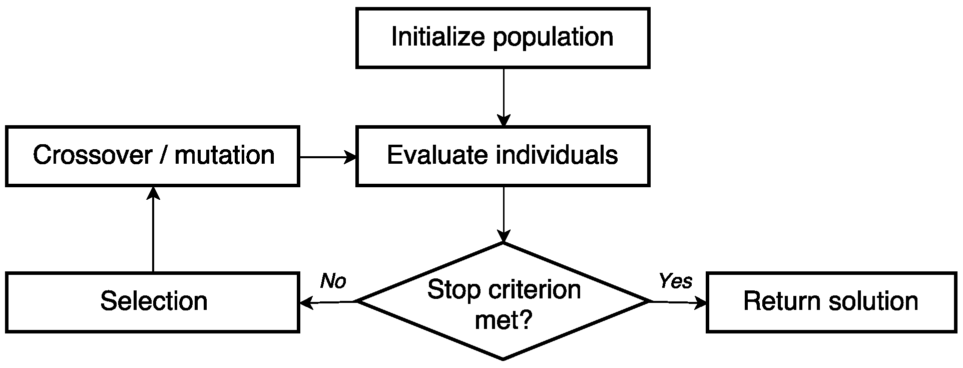
3.1. Background on Genetic Algorithms

Genetic algorithms (GAs) are a stochastic method of intelligent search, where individuals are represented by chromosomes and compete for resources and possibilities for replication. Individuals that are more successful in competitions are more likely to reproduce than those with lower performance. The genes of the individuals evaluated spread well throughout the population, so that they can be improved and can generate increasingly appropriate offspring. The GA algorithm was introduced in [37] and widely popularized through works such as [38].

The GAs are modeled from an optimization problem, in which a trial solution to the problem is constructed in the form of a suitably encoded string of model parameters, called an individual. A collection of individuals is in turn called a population. The main idea of a GA is to evolve toward the best solutions (individuals). Figure 1 shows a simplified scheme of the this evolutionary process. It starts from an initial population of random individuals and continues for many generations. At each generation, the fitness function is used to evaluate the entire population. The fitness function is used to weigh the random selection of several individuals of the current population, which will be modified by variability operations (crossover and mutation) or selection (natural selection and elitism) to form a new population, which will become the current population of the next iteration of the algorithm. When some stopping criterion is met, the best individual found is returned.

3.2. Concepts of Linear Programming Under Uncertainty

Linear programming (LP) is a technique used to optimize linear objective functions, subject to linear equality and linear inequality constraints. A LP can be expressed in canonical form as

$$\begin{array}{cc}\mathrm{Optimize}\hfill & v^{T}w=z\hfill \\ \hfill \mathrm{subject}\mathrm{to}& Uw=b(Uw\le b\mathrm{or}Uw\ge b),U:m\times n,\hfill \\ \hfill & w\ge 0.\hfill \end{array}$$

(1)

where $w\in {\mathbb{R}}^n$ represents the decision variables vector, and v, U and b are known data associated to the problem. The optimization operation can denote either a maximization or a minimization transformation. The mathematical properties of an LP imply in certain assumptions that must be satisfied in relation to the activities of the problem. Thus, these assumptions are defined by [39] as follows:

• Proportionality assumption: The contribution of each activity to the value of the objective function z is proportional to the level of the activity $w_j$, as represented by the $v_j{w}_j$ term in the objective function;
• Additivity assumption: Every function in a linear programming model is the sum of the individual contributions of the respective activities;
• Divisibility assumption: Decision variables in a linear programming model are allowed to have any values, including non-integer values, that satisfy the functional and non-negativity constraints;
• Certainty assumption: The value assigned to each parameter of a linear programming model is assumed to be a known constant.

In real applications, the certainty assumption is seldom satisfied precisely. Linear programming models usually are formulated to select some future course of action. Therefore, the parameter values used would be based on a prediction of future conditions, which inevitably introduces some degree of uncertainty [39]. Thus, a LP model under uncertainty (or a Stochastic Linear Programming) can be defined in a simplified way as

$$\begin{array}{cc}\mathrm{Optimize}\hfill & v^{T}w+E\left[Q(w,\xi )\right]=z\hfill \\ \mathrm{subject}\mathrm{to}\hfill & Uw=b(Uw\le b\mathrm{or}Uw\ge b),U:m\times n,\hfill \\ \hfill & w\ge 0.\hfill \end{array}$$

(2)

where $\xi$ represents the uncertain data and $Q(w,\xi )$ represents the optimal value for the uncertain (stochastic) parameters.

3.3. Adaptive Blind Equalization

3.3.1. Channel Model

A traditional QAM (Quadrature Amplitude Modulation) data transmission system consists of a transmitter, a channel, and a receiver. The channel represents all interconnections between the transmitter and the receiver. An ideal communication channel allows the passage of all the frequency components of the signal, making changes in phase and amplitude as needed. However, in practical situations, communication channels allow only the passage of finite frequency ranges, according to their own physical characteristics. This results in interference between the symbols transmitted by the source, called inter-symbol interference (ISI). In transmission systems whose channel is based on free propagation, the multi-path phenomena are mainly responsible for the appearance of ISI. Figure 2 illustrates in a simplified way the multi-path phenomena, in which each path may be characterized by

$$\begin{array}{c}\hfill {\rho }_i\delta (t-{\tau }_i),\end{array}$$

(3)

where $\delta (·)$ is the impulse function, ${\rho }_i$ is the complex gain (attenuation) of the channel, and ${\tau }_i$ is the delay of the i-th path.

The existence of noise in the communication system can also cause the symbols emitted by the source to be distorted, so that they are not correctly decoded by the receiver. Although it is possible to treat it, it cannot be eliminated from electronic systems [3]. The most common form of noise is thermal noise. Within physical and realization viability, ISI and symbolic distortions caused by noise must be compensated by the receiver.

Figure 3 presents a simplified structure of a discrete base-band digital communication system with ISI, $h\left(k\right)$, thermal noise, $r\left(k\right)$, and a source of information transmitting complex symbols, $a\left(k\right)$, belonging to a M-QAM alphabet, $A=\{a_0,\cdots ,a_{M-1}\}$, of M possible symbols, so that all finite sub-sequences of the M-QAM alphabet symbols occur with non-zero probability. k indicates the discrete time index. The complex symbols, $a\left(k\right)$, are expressed by

$$a\left(k\right)=a^I\left(k\right)+j{a}^Q\left(k\right),$$

(4)

where $a^I\left(k\right)$ and $a^Q\left(k\right)$ are the uni-dimensional phase components and quadrature, respectively, that constitute the bi-dimensional transmitted signal. The symbols $a\left(k\right)$ are transmitted with a sampling period of $T_s$ seconds by means of a channel which is assumed to be linear, causal, BIBO-stable (Bounded-Input Bounded-Output), and in which the impulse response, $h\left(k\right)$, is described as

$${\displaystyle h\left(k\right)={\displaystyle \sum _{i=0}^{L-1}}{\rho }_i\delta (k-{\tau }_i),}$$

(5)

where L is the number of channel paths, ${\rho }_i$ is the complex gain of the i-th path, and ${\tau }_i$ is an integer value representing the i-th path in the instant k. The signal $x\left(k\right)$ represents the signal $a\left(k\right)$ after undergoing channel attenuation. $r\left(k\right)$ represents AWGN so that

$$r\left(k\right)=r^I\left(k\right)+j{r}^Q\left(k\right),$$

(6)

where $r^I\left(k\right)$ and $j{r}^Q\left(k\right)$, respectively, correspond to the phase and quadrature components of AWGN and they are random variables with Gaussian distribution of mean zero and variance ${\sigma }_r^2$ [4]. Then, the equalizer processes the signal $u\left(k\right)$, composed by the channel output, $x\left(k\right)$, and the noise, $r\left(k\right)$, and thus,

$$u\left(k\right)=x\left(k\right)+r\left(k\right),$$

(7)

$${\displaystyle x\left(k\right)={\rho }_0\left(k\right)a(k-{\tau }_0\left(n\right))+{\displaystyle \sum _{i=1}^{L-1}}{\rho }_i\left(k\right)a(k-{\tau }_i\left(k\right)).}$$

(8)

The second term in Equation (8) represents the ISI.

The structure of a blind adaptive equalizer is illustrated in Figure 4, where the output signal is expressed by

$$\begin{array}{ccc}\hfill \tilde{a}(k-d_{eq})& =& {\displaystyle {\displaystyle \sum _{l=0}^{N-1}}{w}_l\left(k\right)u(k-l)}\hfill \\ & =& {\displaystyle {\displaystyle \sum _{l=0}^{N-1}}{w}_l\left(k\right)x(k-l)+{\displaystyle \sum _{l=0}^{N-1}}{w}_l\left(k\right)r(k-l)}\hfill \end{array}$$

(9)

where $w_l$ is the l-th complex gain of the equalizer, N is the equalizer length, and $d_{eq}$ is the equalization delay. The discrete time signals $r\left(k\right)$, $u\left(k\right)$, and $x\left(k\right)$ are expressed by Equations (6), (7), and (8), respectively.

The linear adaptive equalizer (Figure 5) is a linear digital filter (Figure 4), which relies on an algorithm to adapt its parameters, $\mathbf{w}\left(k\right)$, according to the time-varying properties of the communication channel. The adaptation is performed by optimizing a cost function, $J\left(\mathbf{w}\right(k\left)\right)$, in which

$$\begin{array}{ccc}\hfill \mathbf{w}\left(k\right)& =& \left[\begin{array}{c}{w}_0\left(k\right)\\ ⋮\\ w_{N-1}\left(k\right)\end{array}\right]=\left[\begin{array}{c}{w}_0^I\left(k\right)\\ ⋮\\ w_{N-1}^I\left(k\right)\end{array}\right]+j\left[\begin{array}{c}{w}_0^Q\left(k\right)\\ ⋮\\ w_{N-1}^Q\left(k\right)\end{array}\right]\hfill \\ & =& {\mathbf{w}}^I\left(k\right)+j{\mathbf{w}}^Q\left(k\right),\hfill \end{array}$$

(10)

where ${\mathbf{w}}^I\left(k\right)$ and ${\mathbf{w}}^Q\left(k\right)$ are, respectively, real and imaginary parameters of the equalizer.

3.3.2. The Constant Modulus Algorithm

The Constant Modulus Algorithm (CMA), proposed by the authors of [6], is one of the most well-known blind equalization schemes for QAM systems. The CMA cost funtion, $J_{CMA}$, is expressed by

$$J_{CMA}\left(\mathbf{w}\left(k\right)\right)=E\left[e{\left(k\right)}^2\right]$$

(11)

where $E[·]$ denotes statistical expectation, and

$$e\left(k\right)={\displaystyle \frac{E\left\{\right|a_k{|}^{2p}\}}{E\left\{\right|a_k{|}^p\}}}-{\left|\overline{a}\left(k\right)\right|}^p$$

(12)

where $a_k$ is a symbol of the alphabet of the modulation employed. Using the stochastic gradient of the cost function $J_{CMA}$, the filter parameters are updated at each instant k using the stochastic gradient descent rule for the filter coefficients, which is given by

$$\mathbf{w}\left(k\right)=\mathbf{w}(k-1)+\mu e\left(k\right)\mathbf{u}\left(k\right)$$

(13)

where $\mu$ is the adaptation step, and

$$\mathbf{u}\left(k\right)={\left[u\right(k)\cdots u(k-l)\cdots u(K-N+1\left)\right]}^T.$$

(14)

CMA is extremely simple to implement and is able to characterize the level of ISI at the equalizer output regardless of the carrier phase. However, it is highly dependent of the adaptation step being small enough to be stable, and it can lead to a misconvergence due to the existence of local minimum points in the Godard criterion [6,7].

3.3.3. Adaptive Blind Equalization Using Linear Programming

The works [8,9,10] proposed a globally convergent convex cost function based on linear programming. This function does not attempt to directly identify complex channel gain, and instead focuses on eliminating ISI. Once the ISI is removed, the equalizer output becomes a scaled version of the channel input, and it is possible to estimate the scalar gain by simpler methods, such as comparing the input power of the channel with the equalizer output. Thus, the convex cost function for the Blind Linear Equalizer proposed by the above literature can be expressed by

$$J_{PL}\left(\mathbf{w}\right)=J_{PL}\left({\mathbf{w}}^I,{\mathbf{w}}^Q\right)\equiv max\left|{\tilde{a}}^I\left(k\right)\right|+max\left|{\tilde{a}}^Q\left(k\right)\right|.$$

(15)

In this model, it is assumed that the transmitted signal $a\left(k\right)$ is modulated in the scheme M-QAM, with M representing the size of the QAM constellation, and its real and imaginary components are independent and identical, with

$$M\equiv max\left|a^I\left(k\right)\right|=max\left|a^Q\left(k\right)\right|\mathrm{for}\mathrm{any}k,$$

(16)

or they can be transformed to such by rotational operations.

The above model does not take into account the effects of noise, which is impractical in many real-life systems. The work [11] extends the above bibliographies [8,9,10], proving that when considering the effects of AWGN (Additive White Gaussian Noise) in the modeling, the function obtained from Equation (15) remains convex. This proof can be performed by expanding the expression of $\tilde{a}\left(k\right)$ from Equations (7)–(9) and then isolating the terms of $\tilde{a}\left(k\right)$ according to Equation (4), obtaining the expression for ${\tilde{a}}^I\left(k\right)$, given by

$$\begin{array}{ccc}\hfill {\tilde{a}}^I\left(k\right)& =& {\displaystyle \sum _{l=0}^{N-1}}{\displaystyle \sum _{i=0}^{L-1}}\left({\rho }_i^I{a}^I\left(k-{\tau }_i-l\right)\right.\hfill \\ & & \left.-{\rho }_i^Q{a}^Q\left(k-{\tau }_i-l\right)\right)w_l^I\left(k\right)+\hfill \\ & & {\displaystyle \sum _{l=0}^{N-1}}{\displaystyle \sum _{i=0}^{L-1}}\left(-{\rho }_i^I{a}^Q\left(k-{\tau }_i-l\right)\right.\hfill \\ & & \left.-{\rho }_i^Q{a}^I\left(k-{\tau }_i-l\right)\right)w_l^Q\left(k\right)+\hfill \\ & & {\displaystyle \sum _{l=0}^{N-1}}{r}^I(k-l)w_l^I\left(k\right)+{\displaystyle \sum _{l=0}^{N-1}}-r^Q(k-l)w_l^Q\left(k\right).\hfill \end{array}$$

(17)

The term ${\tilde{a}}^Q\left(k\right)$ can be obtained in the same way. The cost function proposed in [8] seeks to minimize the sum of the maximums of the terms of $\tilde{a}\left(k\right)$ (see Equation (15)), which are formed by a sum of linear expressions. Thus, by expanding the terms in evidence of Equation (17), we obtain

$$\begin{array}{ccc}\hfill & & max\left|{\tilde{a}}^I\left(k\right)\right|=\hfill \\ & & max\left|{\displaystyle \sum _{l=0}^{N-1}}{\displaystyle \sum _{i=1}^{L-1}}{\rho }_i^I{a}^I\left(k-{\tau }_i-l\right)w_l^I\left(k\right)\right|\hfill \\ & & +max\left|{\displaystyle \sum _{l=0}^{N-1}}{\displaystyle \sum _{i=0}^{L-1}}-{\rho }_i^Q{a}^Q\left(k-{\tau }_i-l\right)w_l^I\left(k\right)\right|\hfill \\ & & +max\left|{\displaystyle \sum _{l=0}^{N-1}}{\displaystyle \sum _{i=1}^{L-1}}-{\rho }_i^I{a}^Q\left(k-{\tau }_i-l\right)w_l^Q\left(k\right)\right|\hfill \\ & & +max\left|{\displaystyle \sum _{l=0}^{N-1}}{\displaystyle \sum _{i=0}^{L-1}}-{\rho }_i^Q{a}^I\left(k-{\tau }_i-l\right)w_l^Q\left(k\right)\right|\hfill \\ & & +max\left|{\displaystyle \sum _{l=0}^{N-1}}{r}^I(k-l)w_l^I\left(k\right)\right|\hfill \\ & & +max\left|{\displaystyle \sum _{l=0}^{N-1}}-r^Q(k-l)w_l^Q\left(k\right)\right|.\hfill \end{array}$$

(18)

Once again, the terms of $max\left|{\tilde{a}}^Q\left(k\right)\right|$ can be obtained in the same way. It is important to note that Equation (18) is only valid considering that the finite values of the QAM alphabet are limited between $-M$ and $+M$, as defined in Equivalence (16). The functions ${\rho }_i^I{w}_l^I\left(k\right)$, ${\rho }_i^I{w}_l^Q\left(k\right)$, ${\rho }_i^Q{w}_l^I\left(k\right)$, and ${\rho }_i^Q{w}_l^Q\left(k\right)$ are linear in ${\mathbf{w}}^I$ and ${\mathbf{w}}^Q$; their moduli $|{\rho }_i^I{w}_l^I\left(k\right)|$, $|{\rho }_i^I{w}_l^Q\left(k\right)|$, $|{\rho }_i^Q{w}_l^I\left(k\right)|$, and $|{\rho }_i^Q{w}_l^Q\left(k\right)|$ are convex functions in ${\mathbf{w}}^I$ and ${\mathbf{w}}^Q$. Comparing Equation (18) with those presented in [8,9,10], it can be stated that the cost function remains convex in nature, with a different global minimum.

3.4. Blind Linear Equalizer Based on Genetic Algorithms

3.4.1. Architecture

The Blind Linear Equalizer based on genetic algorithm (BLE-GA) is an adaptive blind block equalization scheme whose algorithm uses genetic algorithms as a linear stochastic problem solver. As shown in Figure 6, the BLE-GA operates by storing the received signal, $u\left(k\right)$, in a buffer of length K and then constructing the matrices

$${\mathbf{U}}^I\left(k\right)=[u^I\left(k\right)\cdots u^I(k-K+1)]$$

(19)

and

$${\mathbf{U}}^Q\left(k\right)=[u^Q\left(k\right)\cdots u^Q(k-K+1)].$$

(20)

The vectors ${\mathbf{U}}^I\left(k\right)$ and ${\mathbf{U}}^Q\left(k\right)$ are used by the genetic algorithm to optimize the equalizer weights, $w\left(kK\right)$, in order to perform the channel equalization.

3.4.2. Cost Function

According to the Equation (15), the gains of the K-block equalizer should be adjusted by using the following linear programming strategy:

$$\begin{array}{ccc}\hfill min& & \left\{\begin{array}{c}max\left|{\tilde{a}}^I(k-d_{eq})\right|\\ +max\left|{\tilde{a}}^Q(k-d_{eq})\right|\\ ⋮\\ max\left|{\tilde{a}}^I(k-K+1-d_{eq})\right|\\ +max\left|{\tilde{a}}^Q(k-K+1-d_{eq})\right|,\end{array}\right.\hfill \end{array}$$

(21)

subject to

$$w_{d_{eq}}^I\left(k\right)=1.$$

(22)

This constraint is based on one of the initial conditions of CMA and ensures the equalization of the channel by avoiding the null output, which is the cost function trivial global minimum when $w^I=w^Q=0$. Due to the linear nature of this constraint, neither the convexity nor the global convergence of the cost function are affected.

Substituting the values of ${\tilde{a}}^I(k-d_{eq})$ and ${\tilde{a}}^Q(k-d_{eq})$ for Equation (4), and using the strategy of introducing two auxiliary variables ${\tau }_1$ and ${\tau }_2$, presented earlier in [8,9,10,11], the linear programming strategy presented in Equations (16), (21), and (22) can be expressed by minimizing the following equation:

$$minM{\tau }_1+M{\tau }_2$$

(23)

subject to the following constraints:

$$\begin{array}{ccc}\hfill & & \left\{\begin{array}{c}{\displaystyle {\sum }_{l=0}^{N-1}}{w}_l^I\left(k\right)u^I\left(k-l\right)\\ -w_l^Q\left(k\right)u^Q\left(k-l\right)\le M{\tau }_1\\ ⋮\\ {\displaystyle {\sum }_{l=0}^{N-1}}{w}_l^I\left(k\right)u^I\left(k-l-K+1\right)\\ -w_l^Q\left(k\right)u^Q\left(k-l-K+1\right)\le M{\tau }_1\end{array}\right.\hfill \end{array}$$

(24)

$$\begin{array}{ccc}& & \left\{\begin{array}{c}{\displaystyle {\sum }_{l=0}^{N-1}}{w}_l^I\left(k\right)u^I\left(k-l\right)\\ -w_l^Q\left(k\right)u^Q\left(k-l\right)\ge -M{\tau }_1\\ ⋮\\ {\displaystyle {\sum }_{l=0}^{N-1}}{w}_l^I\left(k\right)u^I\left(k-l-K+1\right)\\ -w_l^Q\left(k\right)u^Q\left(k-l-K+1\right)\ge -M{\tau }_1\end{array}\right.\hfill \end{array}$$

(25)

$$\begin{array}{ccc}& & \left\{\begin{array}{c}{\displaystyle {\sum }_{l=0}^{N-1}}{w}_l^Q\left(k\right)u^I\left(k-l\right)\\ -w_l^I\left(k\right)u^Q\left(k-l\right)\le M{\tau }_2\\ ⋮\\ {\displaystyle {\sum }_{l=0}^{N-1}}{w}_l^Q\left(k\right)u^I\left(k-l-K+1\right)\\ -w_l^I\left(k\right)u^Q\left(k-l-K+1\right)\le M{\tau }_2\end{array}\right.\hfill \end{array}$$

(26)

$$\begin{array}{ccc}\hfill & & \left\{\begin{array}{c}{\displaystyle {\sum }_{l=0}^{N-1}}{w}_l^Q\left(k\right)u^I\left(k-l\right)\\ -w_l^I\left(k\right)u^Q\left(k-l\right)\ge -M{\tau }_2\\ ⋮\\ {\displaystyle {\sum }_{l=0}^{N-1}}{w}_l^Q\left(k\right)u^I\left(k-l-K+1\right)\\ -w_l^I\left(k\right)u^Q\left(k-l-K+1\right)\ge -M{\tau }_2\end{array}\right.\hfill \end{array}$$

(27)

and

$$w_{d_{eq}}^I\left(k\right)=1.$$

(28)

where K represents the number of times the output signal must be stored to construct the optimization curve and $d_{eq}$ is an integer value that represents the equalization delay, so that $0\le d_{eq}\le N-1$. Under the optimum condition, $M{\tau }_1=max\left|{\overline{a}}^I(k-d_{eq})\right|$ and $M{\tau }_2=max\left|{\overline{a}}^Q(k-d_{eq})\right|$. It is important to note that the signal $u\left(k\right)$ is stochastic (see Equation (7)), converting the linear programming problem to a stochastic linear programming problem.

The boundary conditions for Equations (24)–(27) are defined as follows to ensure the validity of the linear constraints under stochastic conditions. For the auxiliary variables ${\tau }_1$ and ${\tau }_2$, the boundaries are set such that $0\le M{\tau }_1,M{\tau }_2\le max\left|a\left(k\right)\right|$, where $a\left(k\right)$ represents the transmitted signal bounded by the modulation alphabet. The equalizer weights ${\mathbf{w}}_I$ and ${\mathbf{w}}_Q$ are constrained to values ensuring that the output signal adheres to the range $[-M,M]$ for each QAM level. Additionally, the condition $w_{d_{eq}}^I\left(k\right)=1$ prevents trivial solutions by ensuring that the equalizer output does not collapse to zero. These conditions are critical to preserving the convexity of the cost function and ensuring robust convergence during optimization.

3.5. Genetic Algorithm Setting

3.5.1. Objective Function

The optimization problem with stochastic linear restrictions to be treated by the genetic algorithm is to minimize $M{\tau }_1+M{\tau }_2$, as defined in Equation (23), subject to the inequality constraints defined by Equations (24)–(27) and to the equality constraint defined by Equation (28).

3.5.2. Encoding

The values to be optimized are the auxiliary variables ${\tau }_1$ and ${\tau }_2$, and the phase and quadrature components of the equalizer weights. Thus, each chromosome is composed of $n=2N+2$ variables (N is the equalizer length) and represented by a double-valued vector $c\left(j\right)$, expressed by

$$c\left(j\right)=[{\tau }_1{\tau }_2{w}_0^I\left(k\right)w_0^Q\left(k\right)\cdots w_{N-1}^I\left(k\right)w_{N-1}^Q\left(k\right)].$$

(29)

where $1\le j\le S$, and S is the population size, which must be suitably chosen to ensure a variety of genes and to avoid affecting the performance of the GA. The problem addressed in this work is a restricted linear problem; therefore, all genes should fit in the hyperspace delimited by all restrictions (Equations (24)–(28)).

3.5.3. Initial Population

The initial population is created by generating random-valued chromosomes that satisfy all bounds and linear constraints. This can be performed by creating many individuals on the boundaries of the constraint region and then creating a well-dispersed population.

3.5.4. Selection and Reproduction Operators

Some qualified individuals are selected for a reproduction operation using the stochastic uniform selection. It is performed by laying out a line in which each parent corresponds to a section of the line of length proportional to its scaled value (evaluated by the objective function described above). The algorithm moves along the line in steps of equal size. At each step, the algorithm allocates a parent from the section it lands on. The first step is a uniform random number less than the step size.

The genetic reproduction operators are the intermediate crossover and the adaptive mutation. The adaptive mutation randomly generates directions that are adaptive with respect to the last successful or unsuccessful generation. The mutation chooses a direction and step length that satisfy bounds and linear constraints. The intermediate crossover creates children by taking a weighted average of the parents. This range ensures the child to be within the boundaries of the constraint region.

These operators were chosen because they can handle optimization problems with constraints. An extended explanation of how these operators work can be found at [40].

4. Methodology

To validate the BLE-GA scheme, several simulations were performed, considering 4-QAM, 16-QAM, and 64-QAM digital communication systems, without channel encoding and operating at a rate of 10 Mbps. These systems were modeled as illustrated in Figure 6. The Matlab software [41] was used to implement and simulate the systems, with the GA-based blind equalization algorithm implemented using the Matlab Optimization Toolbox. The simulations also included an implementation of the CMA in order to have a reference to evaluate the performance of BLE-GA.

Each communication system was evaluated for two scenarios of static channels with ISI and AWGN. These channels, here called Channel A and Channel B, are expressed, respectively, by

$$h_a\left(k\right)=\delta \left(k\right)+0,5\delta (k-3)+0,3\delta (k-6)$$

(30)

and

$$h_b\left(k\right)=\delta \left(k\right)+0,6\delta (k-1)+0,4\delta (k-2).$$

(31)

The simulations performed generated the bit error rate (BER) curves as a function of $E_b/N_0$,

$$E_b={\displaystyle \frac{E\left[a_k^2\right]}{lo{g}_2\left(M\right)}},$$

(32)

where $E_b$ represents the bit energy, and ${\sigma }_r^2$ is the power spectral density of the system noise.

The parameters of the equalizer were adjusted in a period of $T_{ad}$ symbols. After this period ($T_{ad}$ symbols), the error count, i.e., the computation of BER values, started and the equalizer parameters were not updated. The settings employed in the simulations are shown in

Table 2. Parameter setting of the equalizer and CMA.

Parameter	4-QAM	16-QAM	64-QAM
Equalizer length (N)	33	33	33
Equalization delay ($d_{eq}$)	6	6	6
BLE-GA Block length (K)	400	400	1000
CMA Adaptation step ($\mu$)	${10}^{-3}$	${10}^{-3}$	${10}^{-4}$
Adjustment period ($T_{ad}$) in symbols	$1\times {10}^7$	$1\times {10}^7$	$1\times {10}^7$

and

Table 3. Parameter setting of the genetic algorithm. N represents the size of the equalizer.

GA Parameter	Value
Chromosome length	$2N+2$
Crossover fraction	0.9
Elite count	10
Number of Generations	100
Population size	200

. Table 2 presents the parameters for the BLE-GA and CMA equalizers for three modulation schemes: 4-QAM, 16-QAM, and 64-QAM. The selection of the equalizer length N, equalization delay $d_{eq}$, and block length K for BLE-GA, as well as the adaptation step $\mu$ for CMA, was based on extensive empirical testing. These values were optimized to balance each modulation scheme’s convergence speed, computational cost, and equalization accuracy. For instance, the block length K in BLE-GA was adjusted to ensure efficient processing for higher modulation levels, such as 64-QAM, where $K=1000$ symbols were necessary to accommodate increased complexity. Similarly, the adaptation step $\mu$ in CMA was reduced for 64-QAM to maintain stability, reflecting its sensitivity to modulation order. The adjustment period $T_{ad}$ of ${10}^7$ symbols was uniformly set to ensure a fair comparison of the algorithms’ steady-state performance under comparable conditions.

Table 3 details the parameters used for configuring the GA in this study. The parameter N represents the size of the equalizer, directly influencing the chromosome length, which is calculated as $2N+2$. The crossover fraction of 0.9 indicates that 90% of the new population is generated through crossover operations, while the elite count ensures that the top 10 individuals from each generation are preserved. The number of generations (100) and the population size (200) were chosen based on extensive empirical testing to balance convergence speed and computational efficiency. These settings were specifically tailored to optimize the stochastic linear programming cost function described in Section 3.4.2, ensuring effective equalization across varying channel conditions and modulation schemes.

5. Results and Discussion

The results of the simulations concerning channel A, $h_a\left(k\right)$, for the 4-QAM, 16-QAM, and 64-QAM systems are presented, respectively, in Figure 7, Figure 8 and Figure 9. Figure 7 shows a better bit error rate for the 4-QAM system when comparing BLE-GA to the CMA method. In the cases of 16-QAM and 64-QAM systems (Figure 8 and Figure 9), BLE-GA equalized channel A within the period of $T_{ad}=K$ symbols (16-QAM used $K=400$ symbols and 64-QAM used $k=1000$ symbols) in contrast to CMA, which was unable to achieve convergence to a global minimum for the same period. Nevertheless, BLE-GA had a similar performance to CMA when the parameters were adjusted to a much greater period of symbols (4-QAM used $T_{ad}=1\times {10}^3$ symbols, 16-QAM used $T_{ad}=1\times {10}^4$ symbols and 64-QAM used $T_{ad}=7\times {10}^4$ symbols).

The simulations employing the second scenario with channel B, $h_b\left(k\right)$, had nearly similar results to the simulations employing channel A. The $E_b/N_0$ curves for channel B are presented in Figure 10 for the 4-QAM, Figure 11 for 16-QAM and Figure 12 for 64-QAM modulations. The 4-QAM system (see Figure 10) showed slightly higher performance for BLE-GA, gaining up to approximately 2 dB. In the cases of 16-QAM and 64-QAM systems (Figure 11 and Figure 12), BLE-GA provided global convergence, while the CMA method converged to a local minima. CMA performed generally better than BLE-GA when the parameters were adjusted to a greater value of K (4-QAM used $T_{ad}=1\times 700$ symbols, 16-QAM used $T_{ad}=1\times {10}^4$ symbols and 64-QAM used $T_{ad}=1\times {10}^5$ symbols).

The constellation analysis of the equalizer output indicates a substantial performance difference between the BLE-GA equalizer and the CMA equalizer when a signal-to-noise ratio of 30 dB and $T_{ad}=K$ were used. While the BLE-GA equalizer was able to provide visually recognizable constellations (Figure 13a, Figure 14a, Figure 15a, and Figure 16a), the constellations of the CMA equalizer were completely scattered and unrecognizable (Figure 13b, Figure 14b, Figure 15b, and Figure 16b).

In all scenarios, both BLE-GA and CMA converged to global minima, i.e., there was no failure in convergence. However, for $M>4$, CMA required a greater number of iterations to achieve global convergence. For example, in Figure 12 (64-QAM channel B), CMA converged after 100,000 symbols, while BLE-GA required only $1\times {10}^3$ symbols to achieve similar performance.

Another aspect to be taken into account is that BLE-GA is a block channel equalization algorithm. Although BLE-GA is more complex than CMA, it updates the equalizer parameters only after K symbols, while CMA updates them for each symbol. Even if BLE-GA cannot equalize the channel in a K symbol block, it still has a much longer time frame than the CMA to converge to the global minimum.

It is important to note that both methods do not require a training sequence, and they therefore have essentially the same limitation. BLE-GA tries to adjust the constellation of signals within a square with dimensions limited by $\pm M{\tau }_1$ and $\pm M{\tau }_2$, while CMA attempts to adjust the constellation to a radius $\gamma$ [11]. In other words, the challenges are of the same magnitude for both BLE-GA and CMA; therefore, the comparison between these methods is justified. However, BLE-GA does not present the limitations of the CMA of having a cost function with many local minima and relying on the descending gradient method, where convergence is highly dependent on the adaptation step.

6. Conclusions

This paper contributes to the literature with an adaptive blind equalization proposal using a convex optimization technique based on genetic algorithms. The proposed technique is a refinement of earlier work concerning global convergent cost function based on linear programming. It uses genetic algorithms as an optimization technique, which is robust to the stochastic characteristics of the signal to be equalized. An analysis of the BLE-GA performance has been presented, and it shows that the proposed method is more likely to perform better than CMA in greater modulations. However, due to the GA’s complexity, the results of the simulations performed were only possible because of the block architecture of the equalizer, running the GA much fewer times than CMA. The experimental analysis discloses the robustness of the proposed technique as it equalizes channels with proper performance. Thus, the obtained results indicate a significant advancement in the development of efficient algorithms for blind equalization.

References

1. Johnson, R.J.; Schniter, P.; Endres, T.; Behm, J.; Brown, D.; Casas, R. Blind equalization using the constant modulus criterion: A review. Proc. IEEE 1998, 86, 1927–1950. [Google Scholar] [CrossRef]
2. Haykin, S. Communication Systems, 4th ed.; Wiley Publishing: Hoboken, NJ, USA, 2001. [Google Scholar]
3. Haykin, S. Adaptive Filter Theory, 4th ed.; Prentice Hall: Upper Saddle River, NJ, USA, 2001. [Google Scholar]
4. Proakis, J.G. Digital Communications; Mcgraw-Hill College: Upper Saddle River, NJ, USA, 2000. [Google Scholar]
5. Haykin, S. (Ed.) Blind Deconvolution; Prentice Hall: Upper Saddle River, NJ, USA, 1994. [Google Scholar]
6. Godard, D. Self-Recovering Equalization and Carrier Tracking in Two-Dimensional Data Communication Systems. Commun. IEEE Trans. 1980, 28, 1867–1875. [Google Scholar] [CrossRef]
7. Benveniste, A.; Goursat, M. Blind Equalizers. Commun. IEEE Trans. 1984, 32, 871–883. [Google Scholar] [CrossRef]
8. Kennedy, R.A.; Ding, Z. Blind adaptive equalizers for quadrature amplitude modulated communication systems based on convex cost functions. Opt. Eng. 1992, 31, 1189–1199. [Google Scholar] [CrossRef]
9. Ding, Z.; Luo, Z.Q. A fast linear programming algorithm for blind equalization. Commun. IEEE Trans. 2000, 48, 1432–1436. [Google Scholar] [CrossRef]
10. Luo, Z.Q.; Meng, M.; Wong, K.M.; Zhang, J.K. A fractionally spaced blind equalizer based on linear programming. Signal Process. IEEE Trans. 2002, 50, 1650–1660. [Google Scholar] [CrossRef]
11. Fernandes, M.A. Linear programming applied to blind signal equalization. AEU-Int. J. Electron. Commun. 2015, 69, 408–417. [Google Scholar] [CrossRef]
12. Muhammad, M.; Ding, Z. A Linear Programming Receiver for Blind Detection of Full Rate Space-Time Block Codes. IEEE Trans. Signal Process. 2010, 58, 5819–5834. [Google Scholar] [CrossRef]
13. Jacklin, N.; Ding, Z.; Li, Y. On efficient use of pilot symbols for multi-path channel equalization of QAM signals. In Proceedings of the 2013 IEEE International Conference on Communications (ICC), Budapest, Hungary, 9–13 June 2013; pp. 5553–5558. [Google Scholar]
14. Sen, S.; Higle, J.L. An Introductory Tutorial on Stochastic Linear Programming Models. Interfaces 1999, 29, 33–61. [Google Scholar] [CrossRef]
15. Mohammed, J.R. A Study on the Suitability of Genetic Algorithm for Adaptive Channel Equalization. Int. J. Electr. Comput. Eng. (IJECE) 2012, 2, 285–292. [Google Scholar] [CrossRef]
16. Surajudeen-Bakinde, N.; Zhu, X.; Gao, J.; Nandi, A.; Lin, H. Genetic Algorithm Based Frequency Domain Equalization for DS-UWB Systems without Guard Interval. In Proceedings of the 2011 IEEE International Conference on Communications (ICC), Kyoto, Japan, 5–9 June 2011; pp. 1–5. [Google Scholar]
17. Merabti, H.; Massicotte, D. Nonlinear adaptive channel equalization using genetic algorithms. In Proceedings of the 2014 IEEE 12th International New Circuits and Systems Conference (NEWCAS), Trois-Rivieres, QC, Canada, 22–25 June 2014; pp. 209–212. [Google Scholar]
18. Gang, X.; Yourong, L. Blind Equalization Based on a Class of Genetic Algorithms for Wireless Communication. In Proceedings of the 2009 International Forum on Information Technology and Applications, Chengdu, China, 15–17 May 2009; Volume 1, pp. 239–244. [Google Scholar]
19. Han, S.; Pedrycz, W.; Han, C. Nonlinear channel blind equalization using hybrid genetic algorithm with simulated annealing. Math. Comput. Model. 2005, 41, 697–709. [Google Scholar] [CrossRef]
20. Zaouche, A.; Dayoub, I.; Rouvaen, J. Baud-spaced constant modulus blind equalization via hybrid genetic algorithm and generalized pattern search optimization. AEU-Int. J. Electron. Commun. 2008, 62, 122–131. [Google Scholar] [CrossRef]
21. Liu, F.; Ge, L.D.; Wu, Y.J.; Li, J.M. Blind equalization based on immune optimized genetic algorithm. In Proceedings of the 2008 9th International Conference on Signal Processing, Beijing, China, 26–29 October 2008; pp. 1719–1721. [Google Scholar]
22. Lin, H.; Yamashita, K. Hybrid simplex genetic algorithm for blind equalization using {RBF} networks. Math. Comput. Simul. 2002, 59, 293–304. [Google Scholar] [CrossRef]
23. Khafaji, M.J.; Krasicki, M. Uni-Cycle Genetic Algorithm to Improve the Adaptive Equalizer Performance. IEEE Commun. Lett. 2021, 25, 3609–3613. [Google Scholar] [CrossRef]
24. Resende, D.F.; Silva, L.R.M.; Nepomuceno, E.G.; Duque, C.A. Optimizing Instrument Transformer Performance through Adaptive Blind Equalization and Genetic Algorithms. Energies 2023, 16, 7354. [Google Scholar] [CrossRef]
25. Zhou, Q.; Zhang, F.; Yang, C. AdaNN: Adaptive Neural Network-Based Equalizer via Online Semi-Supervised Learning. J. Light. Technol. 2020, 38, 4315–4324. [Google Scholar] [CrossRef]
26. Lauinger, V.; Buchali, F.; Schmalen, L. Blind Equalization and Channel Estimation in Coherent Optical Communications Using Variational Autoencoders. IEEE J. Sel. Areas Commun. 2022, 40, 2529–2539. [Google Scholar] [CrossRef]
27. Murphy, S.L.; Townsend, P.D.; Antony, C. SkipNet: An adaptive neural network equalization algorithm for future passive optical networking. J. Opt. Commun. Netw. 2024, 16, 1082–1092. [Google Scholar] [CrossRef]
28. Wang, Y.; Chang, W.; Li, J.; Yang, C. Signal processing for enhancing railway communication by integrating deep learning and adaptive equalization techniques. PLoS ONE 2024, 19, e0311897. [Google Scholar] [CrossRef] [PubMed]
29. Devrari, A.; Kumar, A.; Kuchhal, P. Global aspects and overview of 5G multimedia communication. Multimed. Tools Appl. 2024, 83, 26439–26484. [Google Scholar] [CrossRef]
30. Hassan, A.Y. A new approach for designing and implementing ADF equalization for 5G frequency selective channel based on two operating phases of LS and RLS algorithms. Telecommun. Syst. 2021, 77, 543–562. [Google Scholar] [CrossRef]
31. Pinchas, M.; Noy, E. A New Blind Adaptive Equalization Method. In Proceedings of the 2022 International Conference on Frontiers of Communications, Information System and Data Science (CISDS), Guangzhou, China, 25–27 November 2022; pp. 128–132. [Google Scholar] [CrossRef]
32. Zhang, L.; Wang, Z.; Zheng, G. OF-FSE: An Efficient Adaptive Equalization for QAM-Based UAV Modulation Systems. Drones 2023, 7, 525. [Google Scholar] [CrossRef]
33. Hu, W.; Wang, Z.; Mei, R.; Lin, M. A Simple and Robust Equalization Algorithm for Variable Modulation Systems. Electronics 2021, 10, 2496. [Google Scholar] [CrossRef]
34. Kumar Mohapatra, P.; Kumar Rout, S.; Kishoro Bisoy, S.; Kautish, S.; Hamzah, M.; Jasser, M.B.; Mohamed, A.W. Application of Bat Algorithm and Its Modified Form Trained with ANN in Channel Equalization. Symmetry 2022, 14, 2078. [Google Scholar] [CrossRef]
35. Chen, Y.; Weng, G.; Luan, S.; Shang, Y.; Liu, C.; Bao, J. Parallel Blind Adaptive Equalization of Improved Block Constant Modulus Algorithm with Decision-Directed Mode. IEEE Access 2023, 11, 85268–85283. [Google Scholar] [CrossRef]
36. Li, J.; Zheng, W.X.; Liu, M.; Chen, Y.; Zhao, N. Robust Blind Equalization for NB-IoT Driven by QAM Signals. IEEE Internet Things J. 2024, 11, 21499–21512. [Google Scholar] [CrossRef]
37. Holland, J.H. Outline for a Logical Theory of Adaptive Systems. J. ACM 1962, 9, 297–314. [Google Scholar] [CrossRef]
38. Goldberg, D.E. Genetic Algorithms in Search, Optimization and Machine Learning, 1st ed.; Addison-Wesley Longman Publishing Co., Inc.: Boston, MA, USA, 1989. [Google Scholar]
39. Hillier, F. Introduction to Operations Research; McGraw-Hill: New York, NY, USA, 2014. [Google Scholar]
40. Matlab. Create Genetic Algorithm Options Structure. 2016. Available online: http://www.mathworks.com/help/gads/gaoptimset.html (accessed on 22 January 2016).
41. Branch, M.; Grace, A. MATLAB Optimization Toolbox: User’s Guide; Computation, Visualization, Programming, MathWorks, Inc.: Natick, MA, USA, 2013. [Google Scholar]
Figure 1. A simplified scheme of the evolutionary process of a GA.
Telecom 06 00006 g001
Figure 2. Multi-path phenomena between transmitter and receiver. ρ i represents the attenuation of the channel, δ ( · ) is the impulse function, and τ i represents the delay of the i-th path.
Telecom 06 00006 g002
Figure 3. Illustration of a discrete base-band communication system with ISI and AWGN. The arrows indicate the transmitted signal ( a ( k ) ), channel response ( h ( k ) ), the output of the channel ( x ( k ) ), the AWGN ( r ( k ) ), the equalizer input ( u ( k ) ), and the equalizer output ( a ( k ) ).
Telecom 06 00006 g003
Figure 4. Structure of a linear equalizer. Variable N represents the length of the equalizer, z 1 indicates a register, u ( k ) indicates the equalizer input, and w ( k ) indicates the parameters of the equalizer.
Telecom 06 00006 g004
Figure 5. Basic scheme of a blind linear adaptive equalizer. The arrows indicate the transmitted signal ( a ( k ) ), the output of the channel ( x ( k ) ), the noise ( r ( k ) ), the equalizer input u ( k ) , the parameters of the equalizer ( w ( k ) ), and the delayed equalizer output ( a ( k d e q ) ).
Telecom 06 00006 g005
Figure 6. Structure of the Blind Linear Adaptive Equalizer based on GA. The arrows indicate the transmitted signal ( a ( k ) ), the output of the channel ( x ( k ) ), the noise ( r ( k ) ), the equalizer input u ( k ) , the parameters of the equalizer ( w ( k ) ), and the delayed equalizer output ( a ( k d e q ) ).
Telecom 06 00006 g006
Figure 7. BER curve of 4-QAM system for channel A. E b / N 0 is expressed in dB.
Telecom 06 00006 g007
Figure 8. BER curve of 16-QAM system for channel A. E b / N 0 is expressed in dB.
Telecom 06 00006 g008
Figure 9. BER curve of 64-QAM system for channel A. E b / N 0 is expressed in dB.
Telecom 06 00006 g009
Figure 10. BER curve of 4-QAM system for channel B. E b / N 0 is expressed in dB.
Telecom 06 00006 g010
Figure 11. BER curve of 16-QAM system for channel B. E b / N 0 is expressed in dB.
Telecom 06 00006 g011
Figure 12. BER curve of 64-QAM system for channel B. E b / N 0 is expressed in dB.
Telecom 06 00006 g012
Figure 13. Constellation diagram of the received signal for the 4-QAM system, using channel A, h a ( k ) (see Equation (30)), with E b / N 0 = 30 dB.
Telecom 06 00006 g013
Figure 14. Constellation diagram of the received signal for the 16-QAM system, using channel A, h a ( k ) (see Equation (30)), with E b / N 0 = 30 dB.
Telecom 06 00006 g014
Figure 15. Constellation diagram of the received signal for the 4-QAM system, using channel B, h b ( k ) (see Equation (31)), with E b / N 0 = 30 dB.
Telecom 06 00006 g015
Figure 16. Constellation diagram of the received signal for the 16-QAM system, using channel B, h b ( k ) (see Equation (31)), with E b / N 0 = 30 dB.
Telecom 06 00006 g016