1. Satellite Constellations with Zenith Propagation Paths at Any Site
Among satellite constellations, the GeoSurf constellations are a good choice for future worldwide internet infrastructure because they share most of the advantages of current GEO (geostationary), MEO (medium Earth orbit) and LEO (low Earth orbit) satellite constellations without suffering most of their drawbacks because they emulate the geostationary orbit with zenith paths in sites located at any latitude [
1].
In [
2], we have compared the tropospheric attenuation of GeoSurf zenith paths with the paths of GEO, MEO and LEO satellites.
In [
3], we have assessed how the annual average probability distribution
of exceeding a given rain attenuation
(dB) depends on the carrier frequency
(GHz) in the GeoSurf paths at sites in different climatic regions. All these studies refer to narrow-band channels, i.e., channels with negligible linear (amplitude and phase) distortions.
In [
4], we have estimated the slowly time-varying transfer function and linear distortions that are likely found in ultra-wideband radio links in GeoSurf constellations working at millimeter wavelengths. As a practical example, the bandwidth considered was 10 GHz wide, centered at 80 GHz (W–Band), because we think it might be used in future worldwide internet radio links using spread spectrum modulation and code division multiple access (CDMA) [
5,
6,
7,
8,
9,
10] with BPSK and QPSK modulation, once high-frequency large wideband technology—now developed at lower frequencies [
11]—will also be available at W-band. CDMA can provide a large processing gain and can be designed without considering issues related to frequency and access coordination which, together with the advantages of the GeoSurf constellations mentioned in Reference [
1], can be an effective choice to provide high bit rates to users.
The literature on what today is defined as “wideband” communication does not refer to rain attenuation or to the ultra-wideband radio links studied here but instead refers only to radio links in clear-sky conditions (mainly multipath), both for terrestrial and satellite systems [
5,
12,
13,
14,
15,
16]; therefore, we discuss these topics further, following work carried out by [
4,
17].
Following our previous study [
4], the purpose of this paper is to assess—with simulations using onsite rain rate time series and the synthetic storm technique (SST) [
18]—the interference due to amplitude and phase distortions produced by rain attenuation in the ultra-wideband communication systems mentioned above and designed for using double sideband-suppressed carrier (DSB-SC) modulation in both quadrature channels (QPSK). We assume that the total signal-to-noise ratio (SNR) of the Gaussian channel is greater than the minimum required to guarantee a bit error probability smaller than the maximum value tolerated by users. Under this hypothesis, we estimate how the in-band attenuation and phase delay affect the baseband digital signal. We evaluate the sampler output of a direct channel (e.g., the cosine channel, inter-symbol interference, ISI) and the quadrature interference (QI) coming from the orthogonal channel (the sine channel, referred to also as the quadrature channel).
For illustrating the characteristics of the interference, we report the results concerning radio links simulated at Spino d’Adda (Italy), Madrid (Spain) and Tampa (Florida), which are sites in different climatic regions (
Table 1). We have considered these specific sites because the rain rate time series
(mm/h)—averaged in 1 min intervals—have been continuously recorded onsite for several years, which is a sufficiently long period to provide reliable experimental results when SST is applied.
The rain fade in GeoSurf radio links is independent of the particular GeoSurf design (e.g., altitude and number of satellites) because all paths to/from a satellite of the constellation are always locally vertical (zenith). To determine the slowly time-varying passband and baseband equivalent transfer functions distorted by rain, we must know the rain attenuation
(dB) and the phase delay
(degrees) time series. Both are calculated with the SST as shown in [
4,
18].
After this introduction,
Section 2 shows examples of the results obtained with the SST;
Section 3 recalls how to calculate passband and baseband transfer functions;
Section 4 reports histograms of interference;
Section 5 models probability distributions of interference;
Section 6 calculates the theoretical channel capacity loss;
Section 7 reports a general conclusion and indicates future work.
2. Rain Attenuation and Phase Delay Due to Rain in Zenith Propagation Paths
To calculate the complex passband (radio frequency) and complex baseband equivalent transfer functions of direct and orthogonal channels in DSB-SC modulation, defined and discussed in [
4] and based on classical linear modulation theory (e.g., [
19,
20]), we must know the time series
(dB) and
(degrees). Both are calculated with the SST [
18], as shown in [
4], with the modelling of [
21,
22,
23].
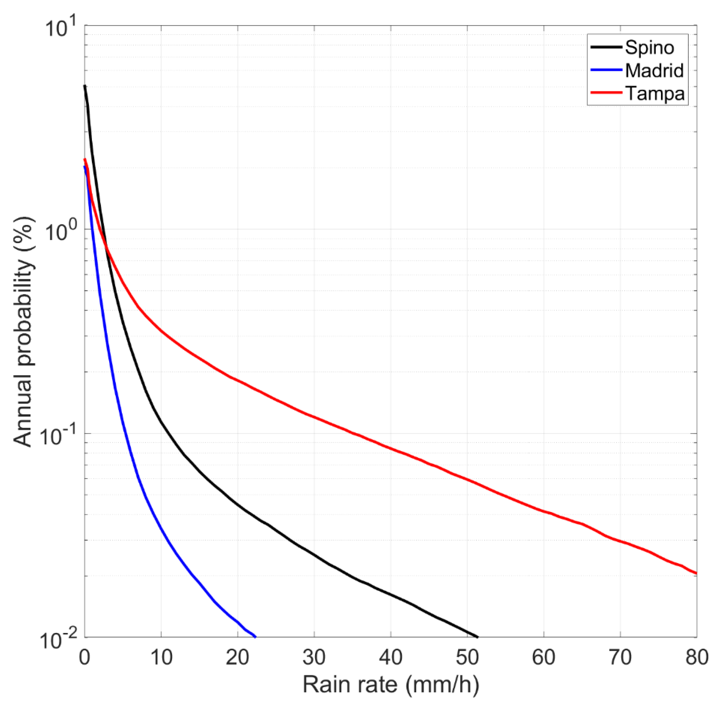
Figure 1 shows the average annual probability distribution
of exceeding
(mm/h, averaged in 1 min) measured at Spino d’Adda, Madrid and Tampa. The different climatic rain conditions at these sites are clearly evident if the rain rates exceeded at equal probability are compared.
Figure 2a shows the annual probability distribution
of exceeding
(dB) calculated with Equation (8) of Reference [
4], and
Figure 2b shows the corresponding annual probability distribution
of exceeding
(degrees) calculated with Equation (9) of Reference [
4].
In the following, we consider the relative phase delay (degrees) at radio frequency
:
We defined the time delay (picoseconds):
where
is measured in GHz and the relative time delay is given by
We defined the normalized magnitude
of the passband transfer function
, at time
as
The real and imaginary parts of
are given by
From Equation (5), according to Reference [
4] (see Equations (5)–(7) of [
4]), we obtain the equivalent baseband complex transfer function of the direct channel as
and the equivalent baseband complex transfer function that couples it to the orthogonal channel:
Now, from
and
, the transfer function can be calculated at any time
, as we will recall in
Section 3. Notice that, since
is averaged in 1 min,
and
are also “averaged” in 1 min, so that the time-varying transfer function changes every minute and, therefore, very slowly compared to any digital signal so that, in every minute, the Gaussian channel is affected by the same in-band rain attenuation and phase delay (see [
4]).
Moreover, we assume that at any time , the channel SNR is larger than the minimum required by the bit error probability constraint; therefore, the rain fade, in order to be compensated with power control or with other techniques, is that which is measured at the highest frequency of the upper side-band, i.e., at 85 GHz in our exercise. Because our purpose is to study transfer functions, we assume the channel is still working as required; in other words, outages are not considered as they are not directly related to transfer functions.
An example illustrates how the SST transforms
into
and
.
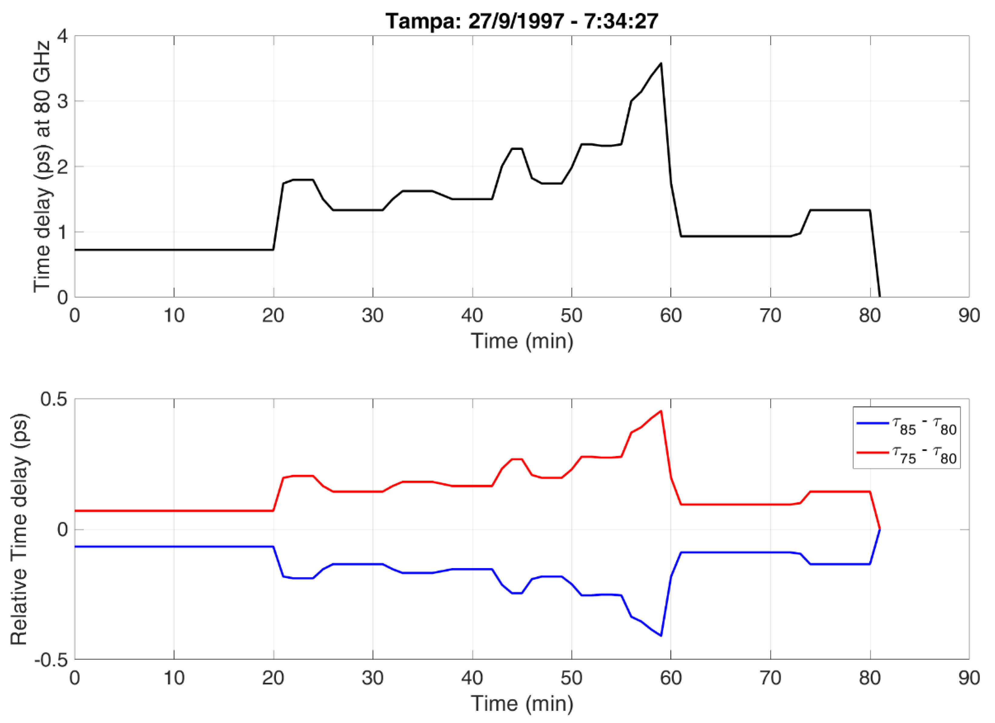
Figure 3 shows
recorded in Tampa and
Figure 4 and
Figure 5 show the corresponding
and the time delay
at 80 GHz and the relative values at the extremes of the 10 GHz bandwidth centered at 80 GHz. Notice that since
and
increase with frequency non–linearly in decibels and in picoseconds, the relative differences are not odd functions.
From these time series, we can calculate the passband and equivalent baseband transfer functions, according to the theory discussed in [
4].
4. Experimental Interference
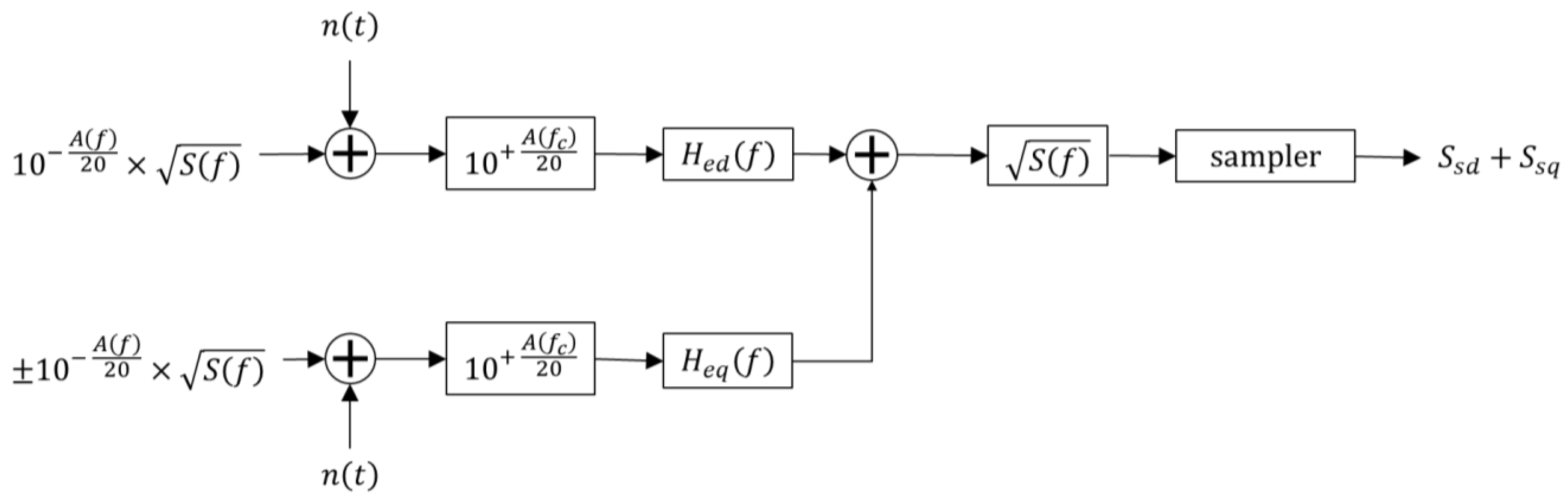
Numerical results have been obtained by means of time-domain simulations of the system described in
Figure 7 in MATLAB/Simulink
®. We have simulated the transmission of a sequence of
symbols drawn from a quadrature phase-shift keying (QPSK) modulation of long sequences of independent bits at the bit rate
(bits per second, bps) according to the value of the roll-off factor
. Since the baseband width is fixed to
GHz, the bit rate is a function of
, given by
We have simulated bit rates corresponding to , i.e., Gbps (gigabits per second); , Gbps; , Gbps. A numerical approximation of the continuous-time square-root Nyquist filter has been implemented by considering a windowing of 16 symbol intervals and an oversampling factor of 4 compared to the symbol rate.
Because we refer to normalized values, the algebraic sum of total interference
gives the factor by which the SNR
obtainable in the ideal channel (
Figure 6) must be multiplied to obtain the SNR in the presence of ISI and QI. Therefore, we defined the channel factor
:
The SNR obtainable with interference is given by
In applying these equations, we assume that the channel Gaussian noise power is constant, although it should slightly increase with rain attenuation.
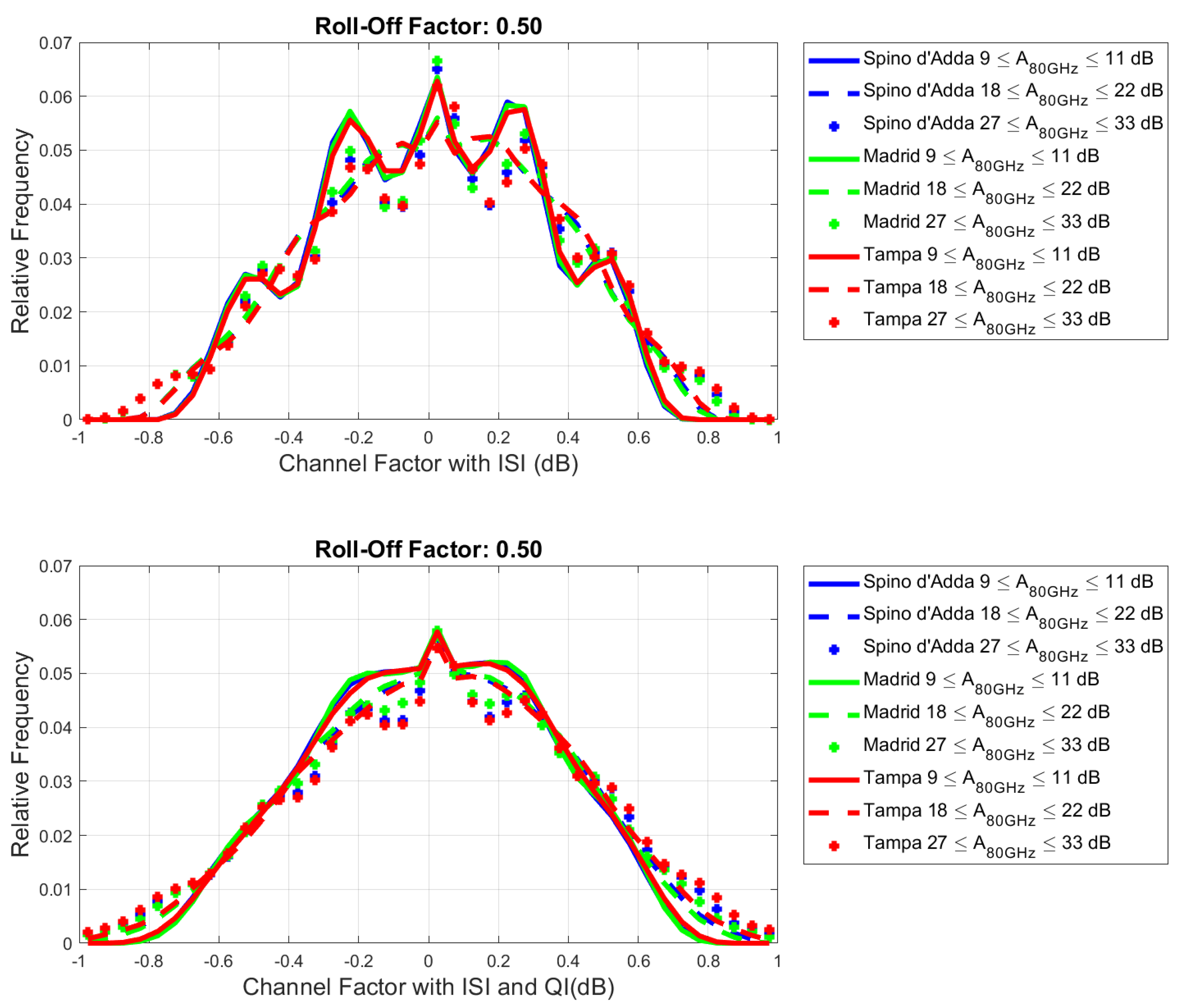
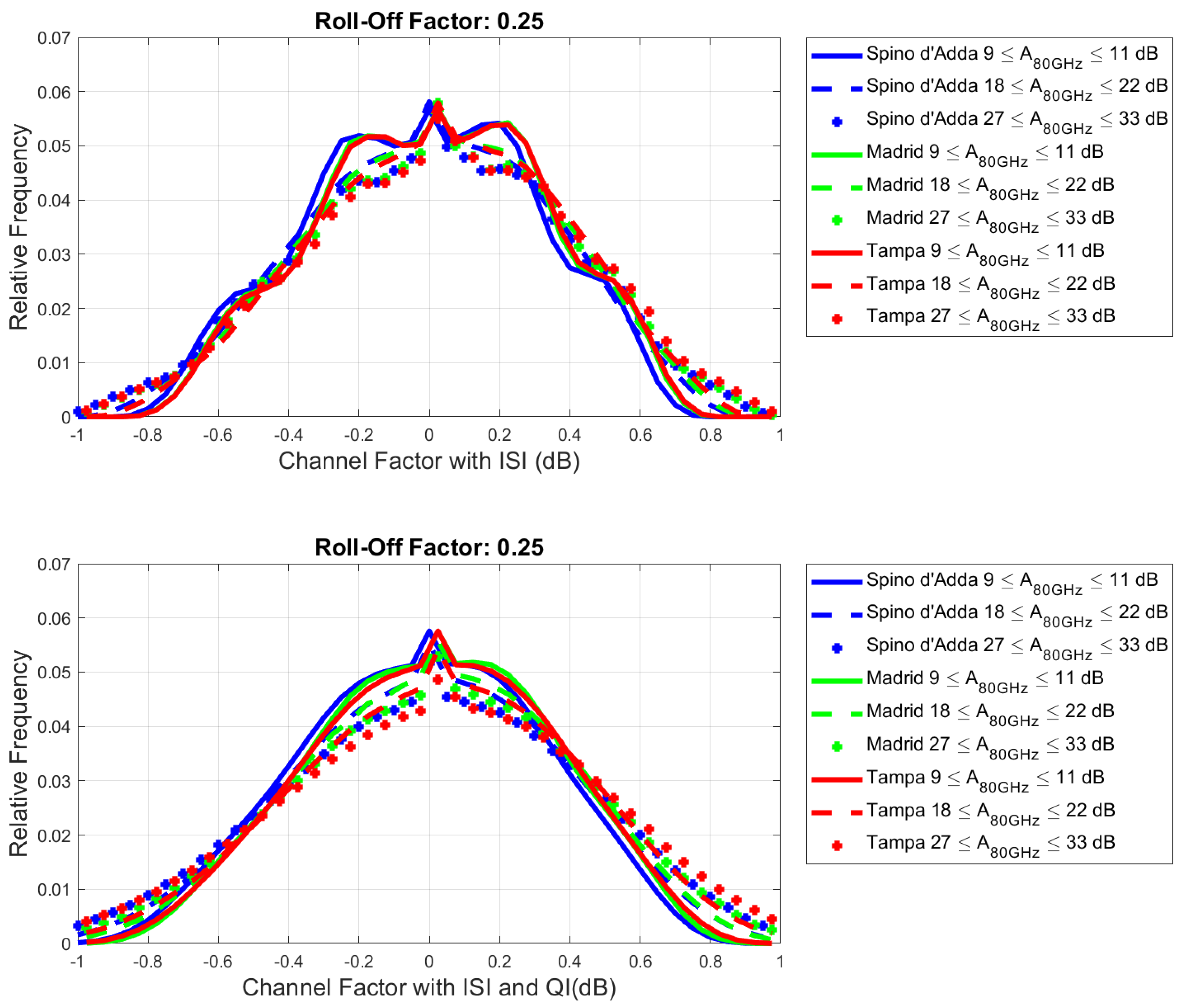
Our main results are the histograms (relative frequency) of the sampler output amplitude (dB) first but only with ISI and then only with ISI and QI, i.e., with the total interference. To show the dependence on the rain attenuation calculated at the center frequency (i.e., 80 GHz), we have considered the cases in which rain attenuation (and corresponding time delay) was in the following ranges: dB (referred to, for short, as “10” dB), dB (“20” dB) and dB (“30” dB).
Figure 8 shows the relative frequency histogram of the channel factor
(dB) for
,
Figure 9 for
and
Figure 10 with
.
From these results, we can draw the following general conclusions:
- (1)
The three sites, although in different climatic zones, are practically indistinguishable in all cases.
- (2)
All histograms show even symmetry; therefore, indicating that for about 50% of the time, we can consider the channel factor to be either (dB), therefore, ; or (dB), therefore, .
- (3)
Histograms with only ISI and with ISI + QI are distinguishable.
- (4)
With ISI only, the lowest range of attenuation (10 dB) shows more marked peaks at dB and dB. These peaks are largely smoothed when QI is also added.
- (5)
The roll-off factor plays a small role because the values of the peaks change a little, especially for .
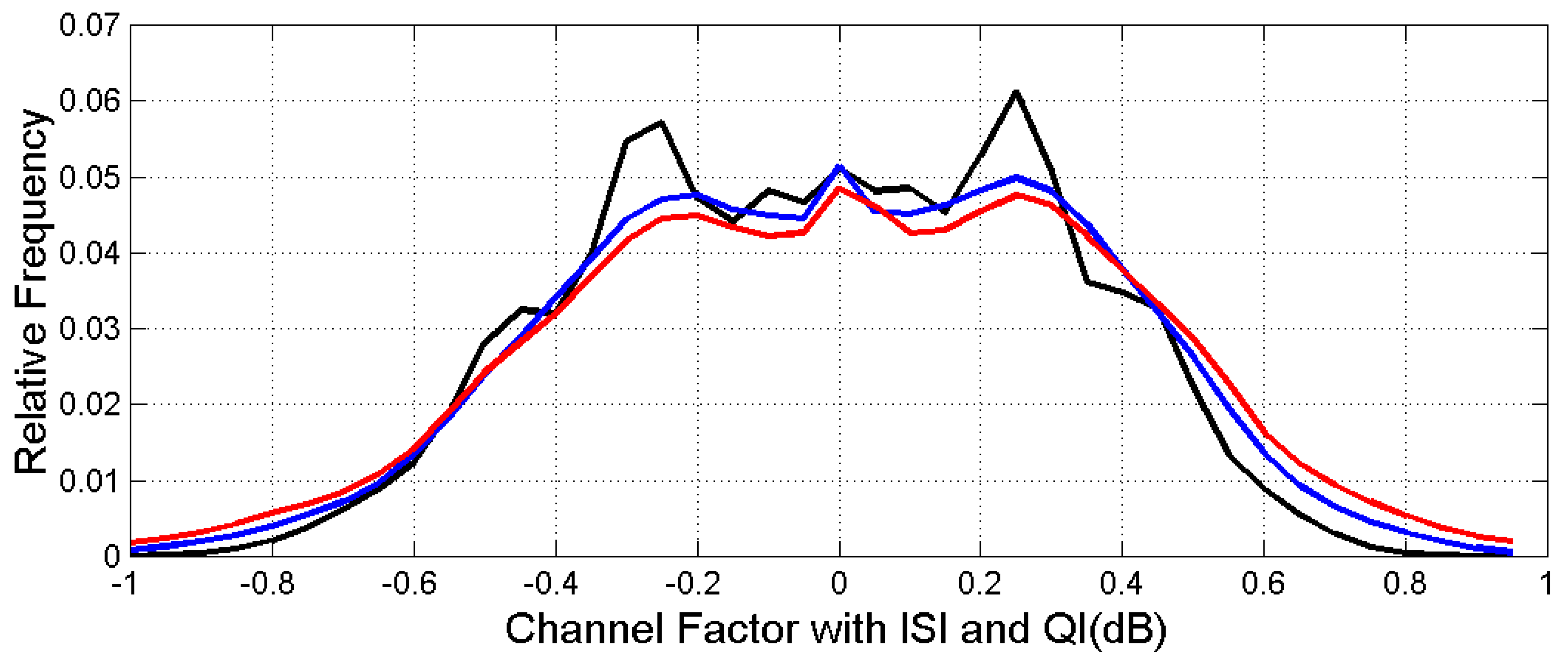
Because of these general findings, in
Figure 11, we have drawn the average relative frequency histograms by distinguishing only the three attenuation ranges. In other words, this figure should provide a “global” frequency distribution of the channel factor in a 10 GHz bandwidth centered at 80 GHz. In the next section, we will propose a theoretical approach which can justify these findings.
Author Contributions
Conceptualization, E.M., M.M. and C.R.; methodology, E.M., M.M. and C.R.; software, E.M., M.M. and C.R.; investigation, E.M., M.M. and C.R.; data curation, E.M., M.M. and C.R.; writing—original draft preparation, E.M., M.M. and C.R.; writing—review and editing, E.M., M.M. and C.R.; visualization, E.M., M.M. and C.R. All authors have read and agreed to the published version of the manuscript.
Funding
This research received no external funding.
Data Availability Statement
Not applicable.
Acknowledgments
We wish to thank Roberto Acosta, at NASA years ago, for providing the rain rate data of Tampa and we also wish to thank José Manuel Riera, at the Universidad Politécnica de Madrid, for providing the rain rate data of Madrid.
Conflicts of Interest
The authors declare no conflict of interest.
References
- Matricciani, E. Geocentric Spherical Surfaces Emulating the Geostationary Orbit at Any Latitude with Zenith Links. Future Internet 2020, 12, 16. [Google Scholar] [CrossRef]
- Matricciani, E.; Riva, C.; Luini, L. Tropospheric Attenuation in GeoSurf Satellite Constellations. Remote Sens. 2021, 13, 5180. [Google Scholar] [CrossRef]
- Matricciani, E.; Riva, C. Outage Probability versus Carrier Frequency in GeoSurf Satellite Constellations with Radio–Links Faded by Rain. Telecom 2022, 3, 504–513. [Google Scholar] [CrossRef]
- Matricciani, E.; Riva, C. Transfer–functions and Linear Distortions in Ultra–Wideband Channels Faded by Rain in GeoSurf Satellite Constellations. Future Internet 2023, 15, 27. [Google Scholar] [CrossRef]
- Kennedy, R.S. Fading Dispersive Communication Channels; Wiley: New York, NY, USA, 1969. [Google Scholar]
- Turin, G.L. Introduction to spread spectrum antimultipath techniques and their application to urban digital radio. Proc. IEEE 1980, 68, 328–353. [Google Scholar]
- Pickholtz, R.; Schilling, D.; Milstein, L. Theory of spread–spectrum communications—A tutorial. IEEE Trans. Commun. 1982, 30, 855–884. [Google Scholar]
- Viterbi, A.J. CDMA Principles of Spread Spectrum Communications; Addinson–Wesly: Reading, MA, USA, 1995. [Google Scholar]
- Dinan, E.H.; Jabbari, B. Spreading codes fir direct sequence CDMA and wideband CDMA celluar networks. IEEE Commun. Mag. 1998, 36, 48–54. [Google Scholar] [CrossRef]
- Veeravalli, V.V.; Mantravadi, A. The coding–spreading trade–off in CDMA systems. IEEE Trans. Sel. Areas Commun. 2002, 20, 396–408. [Google Scholar] [CrossRef]
- Matsusaki, Y.; Masafumi, N.; Suzuki, Y.; Susumu, N.; Kamei, M.; Hashimoto, A.; Kimura, T.; Tanaka, S.; Ikeda, T. Development of a Wide–Band Modem for a 21–GHz Band Satellite Broadcasting System. In Proceedings of the 2014 IEEE Radio and Wireless Symposium (RWS), Newport Beach, CA, USA, 19–23 January 2014. [Google Scholar]
- Parsons, D. The Mobile Radio Propagation Channel; Wiley: New York, NY, USA, 1994. [Google Scholar]
- Simon, M.K.; Alouini, M.S. Digital Communication over Fading Channels: A Unified Approach to Performance Analysis; Wiley: New York, NY, USA, 2000. [Google Scholar]
- Greenstein, L.G.; Andersen, J.B.; Bertoni, H.L.; Kozono, S.; Michelson, D.G. (Eds.) Special Issue on Channel and Propagation Modeling for Wireless Systems Design. J. Sel. Areas Commun. 2002, 20. [Google Scholar] [CrossRef]
- Goldsmith, A. Wireless Communications; Cambridge University Press: Cambridge, NY, USA, 2005. [Google Scholar]
- Pérez–Fontan, F.; Pastoriza–Santos, V.; Machado, F.; Poza, F.; Witternig, N.; Lesjak, R. A Wideband Satellite Maritime Channel Model Simulator. IEEE Trans. Antennas Propag. 2022, 70, 214–2127. [Google Scholar] [CrossRef]
- Matricciani, E. A Relationship between Phase Delay and Attenuation Due to Rain and Its Applications to Satellite and Deep–Space Tracking. IEEE Trans. Antennas Propag. 2009, 57, 3602–3611. [Google Scholar] [CrossRef]
- Matricciani, E. Physical–mathematical model of the dynamics of rain attenuation based on rain rate time series and a two–layer vertical structure of precipitation. Radio Sci. 1996, 31, 281–295. [Google Scholar] [CrossRef]
- Schwartz, M. Information, Transimission, Modulation and Noise, 4th ed.; McGraw–Hill Int. Ed.: New York, NY, USA, 1990. [Google Scholar]
- Carassa, F. Comunicazioni Elettriche; Bollati Boringhieri: Turin, Italy, 1978. [Google Scholar]
- Matricciani, E. Rain attenuation predicted with a two–layer rain model. Eur. Tranactions Telecommun. 1991, 2, 715–727. [Google Scholar] [CrossRef]
- Recommendation ITU–R P.839–4. Rain Height Model for Prediction Methods; ITU: Geneva, Switzerland, 2013. [Google Scholar]
- Maggiori, D. Computed transmission through rain in the 1–400 GHz frequency range for spherical and elliptical drops and any polarization. Alta Frequenza. 1981, 50, 262–273. [Google Scholar]
- Papoulis, A. Probability & Statistics; Prentice Hall: Hoboken, NJ, USA, 1990. [Google Scholar]
- Lindgren, B.W. Statistical Theory, 2nd ed.; MacMillan Company: New York, NY, USA, 1968. [Google Scholar]
Figure 1.
Annual probability distribution (%) of exceeding the value indicated in abscissa at Spino d’Adda, Madrid and Tampa.
Figure 2.
(a) Annual probability distribution (%) of exceeding the value indicated in abscissa at Spino d’Adda, Madrid and Tampa; (b) annual probability distribution (%) of exceeding the value indicated in abscissa at Spino d’Adda, Madrid and Tampa, at 80 GHz and with circular polarization.
Figure 3.
Rain rate time series recorded at Tampa on 27 September 1997. According to the rain gauge collecting rainfall, the rain event started at 7:34:27 AM, local time. Samples are averaged in 1 min.
Figure 4.
SST simulated event at Tampa, 27 September 1997, started at 7:34:27 AM local time. (Upper panel): rain attenuation (dB) at 80 GHz (circular polarization). (Lower panel): relative attenuation at the extremes of a 10 GHz bandwidth. Sampling time is 1 min.
Figure 5.
SST simulated event at Tampa, 27 September 1997, started at 7:34:27 AM, local time. (Upper panel): phase delay (picoseconds) at 80 GHz (circular polarization). (Lower panel): relative phase delay at the extremes of a 10 GHz bandwidth. Sampling time is 1 min.
Figure 6.
Flowchart of the baseband receiver in ideal conditions. is the two-sided spectrum of the Nyquist pulse, is its matched filter, is the receiver total additive Gaussian white noise.
Figure 7.
Flowchart of the quadrature baseband receiver in rain attenuation. is the two-sided spectrum of the Nyquist reference pulse assumed to be positive, is the matched filter and is the receiver total additive Gaussian white noise for each channel of equal power.
Figure 8.
Relative frequency histogram of the channel factor (dB) with ISI (upper panel) and with ISI and QI (lower panel). Color key: blue = Spino d’Adda; green = Madrid; red = Tampa. Curve key: continuous dB; dashed dB; “+” dB. Roll-off factor .
Figure 9.
Relative frequency histogram of the channel factor (dB) with ISI (upper panel) and with ISI and QI (lower panel). Color key: blue = Spino d’Adda; green = Madrid; red = Tampa. Curve key: continuous dB; dashed dB; “+” dB. Roll-off factor .
Figure 10.
Relative frequency histogram of the channel factor (dB) with ISI (upper panel) and with ISI and QI (lower panel). Color key: blue = Spino d’Adda; green = Madrid; red = Tampa. Curve key: continuous dB; dashed dB; “+” dB. Roll-off factor .
Figure 11.
Average relative frequency histogram of the channel factor (dB) in the presence of ISI and QI. Curve key: black ; blue ; red . Curves are averaged over the sites and roll-off factors.
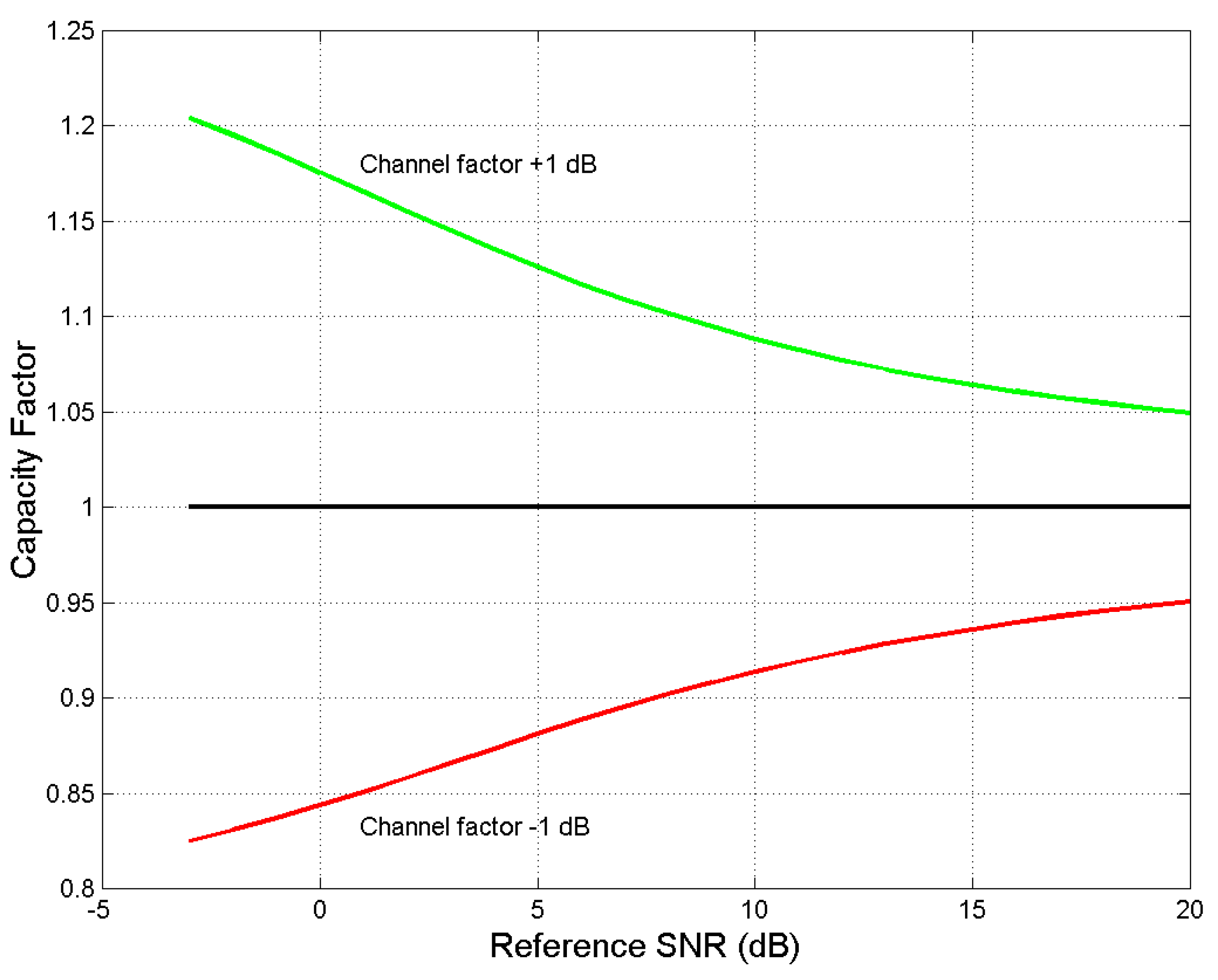
Figure 12.
Capacity factor versus
(dB) at the extreme values of
; namely,
dB. The experimental values of
Figure 10,
Figure 11 and
Figure 12 are within these bounds.
Table 1.
Geographical coordinates, altitude (km), rain height (km), number of years of continuous rain rate time series measurements at the indicated sites.
| Site | Latitude N (°) | Longitude E (°) | Altitude (km) | Precipitation Height (km) | Rain Rate Data Bank (Years) |
|---|
| Spino d’Adda (Italy) | 45.4 | 9.5 | 0.084 | 3.341 | 8 |
| Madrid (Spain) | 40.4 | 356.3 | 0.630 | 3.001 | 8 |
| Tampa (Florida) | 28.1 | 277.6 | 0.050 | 4.528 | 4 |
| Disclaimer/Publisher’s Note: The statements, opinions and data contained in all publications are solely those of the individual author(s) and contributor(s) and not of MDPI and/or the editor(s). MDPI and/or the editor(s) disclaim responsibility for any injury to people or property resulting from any ideas, methods, instructions or products referred to in the content. |
© 2023 by the authors. Licensee MDPI, Basel, Switzerland. This article is an open access article distributed under the terms and conditions of the Creative Commons Attribution (CC BY) license (https://creativecommons.org/licenses/by/4.0/).


