Call Blocking Probabilities under a Probabilistic Bandwidth Reservation Policy in Mobile Hotspots

Abstract

In this paper we study a mobility-aware call admission control algorithm in a mobile hotspot. To this end, a vehicle is considered which has an access point with a fixed capacity. The vehicle alternates between stop and moving phases. When the vehicle is in the stop phase, it services new and handover calls by prioritizing them via a probabilistic bandwidth reservation (BR) policy. Based on this policy, new handover calls may enter the reservation space with a predefined probability. When the vehicle is in the moving phase, it services new calls only. In that phase, two different policies are considered: (a) the classical complete sharing (CS) policy, where new calls are accepted in the system whenever there exists available bandwidth, and (b) the probabilistic BR policy. Depending on the selected policy in the moving phase, we propose the probabilistic BR loss model (if the CS policy is selected) and the generalized probabilistic BR loss model (if the probabilistic BR policy is selected). In both stop and moving phases, where the call arrival process is Poisson, calls require a single bandwidth unit in order to be accepted in the system, while the service time is exponentially distributed. To analytically determine call blocking probabilities and the system’s utilization, we propose efficient iterative algorithms based on two-dimensional Markov chains. The accuracy of the proposed algorithms is verified via simulation.

1. Introduction

Call admission control (CAC) is a significant quality of service (QoS) mechanism in contemporary networks, not only because it controls the access to the bandwidth units (b.u.) required by new mobile users but also because it provides fairness among different mobile applications and at the same time affects the QoS of in-service calls [1,2,3,4].

Considering call-level traffic in wireless networks, such a QoS mechanism is a resource sharing policy that affects call blocking probabilities (CBP) of both new and handover calls. The term CBP refers to the blocking of new or handover calls due to the unavailability of b.u. To reduce CBP (especially of handover calls), various bandwidth sharing policies exist in the literature, with the most common being the guard channel or bandwidth reservation (BR) policy [5,6,7,8,9,10,11,12]. The main characteristic of the BR policy is that it introduces a priority to handover calls by reserving b.u. in favor of them. On the other hand, such a reservation usually results in a significant CBP increase of new calls [13,14,15,16].

We focus on a CAC mechanism proposed in [7] that is based on the BR policy and is applied on a mobile hotspot. The work of [7] considers a vehicle that has an access point (AP) installed on it with a wireless local area network (WLAN) capacity of $C$ b.u. The vehicle can be in two different phases: (a) in the stop phase and (b) in the moving phase. During the stop phase, a vehicle remains in a location (e.g., a station area) and can accommodate two different types of users: new and handover users. New users may initiate a call when they enter the vehicle. On the other hand, handover users have an ongoing call and perform a handover from a NodeB (NB) to the vehicle’s AP. To favor handover users, in terms of reduced CBP, a part of the C b.u. is reserved for them. During the moving phase, only new calls can be generated. To this end, two policies have been studied in that phase. They are: (i) the classical complete sharing (CS) policy, where b.u. are provided to a new call if they exist at the time of the call’s arrival, and (ii) the BR policy, where a part of the C b.u. cannot be accessed by new calls (although handover calls are not generated during the moving phase), a fact that substantially increases the CBP of new calls. In both phases, calls require a single b.u., follow a Poisson process and have an exponentially distributed service time. The main target of [7] is the CBP determination in the stop and moving phases, as well as the computation of the system’s utilization with the aid of a 2-D Markov chain analysis. The reason behind the usage of a two-dimensional Markov chain lies in the fact that two phases (the stop and the moving) exist in the model and interact with each other. A model similar to [7] has been proposed in [6] and recently improved in [17]. In [6,17], the stop and moving phases are treated independently. Such a fact simplifies the corresponding Markov chains as well as the necessary analytical CBP calculations (which are based on the classical Erlang B formula [18,19]), but may lead to analytical CBP results that are not always close to the corresponding simulation results. The idea of the stop-moving phases may also be considered for the CBP determination in the more demanding framework of high-speed railway communications, but this is still an open research issue [20,21,22].

In this paper, we extend the work of [7] by proposing a probabilistic BR policy that can be applied to new calls (either in the stop or in the moving phase) with a predefined probability that can be different for each phase. The reason behind studying such a probabilistic BR policy is the following: when the “strict” BR policy is applied to prioritize a certain type of call, it can lead to a substantial CBP increase in other types of calls that share the same b.u. [17,18,19,23,24]. To this end, the advantage of adopting such a policy, compared to the classical CS and “strict” BR policies, is that it provides a flexible way to alter CBP of both new and handover calls by changing the BR policy probabilities. Besides, it is significant, from an engineering point of view, to have a simple and yet efficient algorithm for the computation of CBP under the probabilistic BR policy. Note that such an algorithm has not been presented in [7] for the determination of CBP.

Based on the above, the contribution of our paper is summarized as follows: (i) we propose the probabilistic BR loss model where the probabilistic BR policy is applied only to new calls during the stop phase; (ii) we propose an iterative algorithm for the determination of the steady-state probabilities that are essential for the computation of the various performance measures (CBP and system’s utilization); (iii) we extend the previous model by proposing the generalized probabilistic BR loss model, where the probabilistic BR policy is applied to new calls in both stop and moving phases; and (iv) we propose an iterative algorithm for the computation of the steady-state probabilities and the various performance measures.

This paper is organized as follows: In Section 2, we propose the probabilistic BR loss model, describe the analytical model (Section 2.1), propose an iterative algorithm for the determination of the steady-state probabilities (Section 2.2) and propose formulas for the determination of the various performance measures (Section 2.3). In Section 3, we propose the generalized probabilistic BR loss model. In Section 4, we present simulation and analytical results so as to validate the accuracy of the proposed formulas. We conclude in Section 5. In Appendix A, a tutorial example is presented with the intermediate calculations of the iterative algorithm in the probabilistic BR loss model. Finally, the abbreviations and notation used in this paper are listed at the end, respectively.

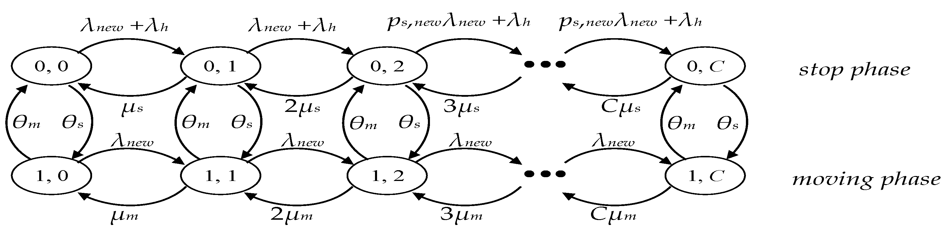
2. The Probabilistic BR Loss Model

2.1. The Analytical Model

Consider a vehicle with an AP installed on it and let the capacity of the AP’s WLAN be equal to C b.u. The CAC proposed in [7] considers two different phases regarding the vehicle: a stop phase and a moving phase.

During the stop phase, the vehicle remains for an exponentially distributed time in a location (e.g., a bus stop or a bus station), with mean ${\theta }_s^{-1}$, and can accommodate Poisson arriving calls. The latter requests a single b.u. in order to be accepted in the system. If this b.u. is not available then an arriving call is blocked and lost without further affecting the system. Two types of users are considered during the stop phase: (1) new users who initiate a call after riding on the vehicle and (2) handover users who already have an ongoing call and should perform a handover from a NB to the vehicle’s AP. To facilitate handover users, the probabilistic BR policy is considered whereby t_new b.u. are reserved for them. This means that a prioritization is applied to handover calls since they are blocked only if all C b.u. are occupied while a new call is blocked: (i) with a predefined probability (1 − p_s,new) when the occupied b.u. j = C − t_new, …, C − 1 and (ii) with probability 1 when the occupied b.u. j = C. Note that in the case of the “strict” BR policy, the value of p_s,new = 0 when j = C − t_new, …, C − 1. The reason behind such a probabilistic BR policy is the following: when the “strict” BR policy is applied to prioritize a certain type of call, it can lead to a substantial CBP increase of the other types of calls that share the same link. In our case, the introduction of a probabilistic BR policy and the proper selection of p_s,new can protect new calls from such a substantial CBP increase. As a last comment, note that if t_new = 0 then p_s,new = 1, i.e., new calls are allowed to have access in all C b.u.

During the moving phase, the vehicle moves from one location to another. We assume that the duration of the moving phase is also exponentially distributed with mean ${\theta }_m^{-1}$. In the moving phase, handover calls (from the NB to the vehicle’s AP) cannot be generated and therefore only new calls should be considered. Consequently, there is no reason to adopt the BR policy in that phase. More specifically, during a moving phase, the CS policy is adopted.

Let λ_new and λ_h be the arrival rate for Poisson arriving new and handover calls, respectively. Accepted calls remain in the system for an exponentially distributed service time, with mean ${\mu }_s^{-1}$ in the stop phase and ${\mu }_m^{-1}$ in the moving phase.

The proposed analytical model can be described as a 2-D Markov chain, whose state space diagram is depicted in Figure 1, assuming for illustration purposes that the reservation space starts in state (0,2). Based on this chain, let P(i,n) be the steady-state probability that the vehicle is in phase i (i = 0 refers to the stop phase and i = 1 refers to the moving phase) and there exist n users in-service, where $0\le n\le C$.

We initially consider the global balance equations for the boundary states (0,0) and (1,0):

$$\begin{array}{l}\mathrm{state} (0,0): ({\lambda }_{new}+{\lambda }_h+{\theta }_s)P(0,0)-{\mu }_{s}P(0,1)-{\theta }_{m}P(1,0)=0\hspace{1em}\hspace{1em}\hspace{1em}(for i=0,n=0)\\ \mathrm{state} (1,0): ({\lambda }_{new}+{\theta }_m)P(1,0)-{\mu }_{m}P(1,1)-{\theta }_{s}P(0,0)=0\hspace{1em}\hspace{1em}\hspace{1em}\hspace{1em}(fori=1,n=0)\end{array}$$

or in a more compact way:

$$({\lambda }_i(0)+{\theta }_i)P(i,0)-{\mu }_{i}P(i,1)-{\theta }_{j}P(j,0)=0$$

(1)

where ${\lambda }_i(0)=\{\begin{array}{l}{\lambda }_{new}+{\lambda }_h, i=0\\ {\lambda }_{new} , i=1\end{array}, {\theta }_i(0)=\{\begin{array}{l}{\theta }_s , i=0\\ {\theta }_m, i=1\end{array} , {\mu }_i=\{\begin{array}{l}{\mu }_s , i=0\\ {\mu }_m, i=1\end{array} , j=1-i.$

We consider now the states below the system’s capacity, i.e., the states where 0 < n < C. For these states, the following global balance equation can be written:

$$({\lambda }_i(n)+n{\mu }_i+{\theta }_i)P(i,n)-{\lambda }_i(n-1)P(i,n-1)-{\theta }_{j}P(j,n)-(n+1){\mu }_{i}P(i,n+1)=0$$

(2)

where ${\lambda }_i(n)=\{\begin{array}{l}{\lambda }_{new}+{\lambda }_h, i=0, 0<n\le C-t_{new}-1\\ p_{s,new}{\lambda }_{new}+{\lambda }_h, i=0, C-t_{new}\le n<C\\ {\lambda }_{new}, i=1, 0<n<C\end{array}, j=1-i.$

Finally, we consider the boundary states (0,C) and (1,C). For these states, we have the following global balance equation:

$$(C{\mu }_i+{\theta }_i)P(i,C)-{\lambda }_i(C-1)P(i,C-1)-{\theta }_{j}P(j,C)=0$$

(3)

To determine the values of P(i,n) based on (1)–(3), an iterative algorithm is proposed in the following subsection.

2.2. An Iterative Algorithm for the Determination of P(i,n)

Initially, we express P(i,n) via the boundary states P(0,0) and P(1,0) as follows:

$$P(i,n)=S_{i,n}^{0}P(0,0)+S_{i,n}^{1}P(1,0)$$

(4)

At this point, all terms in (4) (including the coefficients $S_{i,n}^0$ and $S_{i,n}^1$) are unknown. A formula for the derivation of $S_{i,n}^0$ and $S_{i,n}^1$ can be obtained if we substitute (4) in (2), to have:

$$\begin{array}{ll}{S}_{i,n+1}^{0}P(0,0)+S_{i,n+1}^{1}P(1,0)& =\frac{{\lambda }_i(n)+n{\mu }_i+{\theta }_i}{(n+1){\mu }_i}\left(S_{i,n}^{0}P(0,0)+S_{i,n}^{1}P(1,0)\right)-\frac{{\lambda }_i(n-1)}{(n+1){\mu }_i}\left(S_{i,n-1}^{0}P(0,0)+S_{i,n-1}^{1}P(1,0)\right)\\ & -\frac{{\theta }_j}{(n+1){\mu }_i}\left(S_{j,n}^{0}P(0,0)+S_{j,n}^{1}P(1,0)\right),\end{array}$$

(5)

where j = 1−i.

To determine the values of $S_{i,n}^0$ in (5), we assume that P(0,0) = 1 and P(1,0) = 0. Based on (5), we have the following recursive formula:

$$S_{i,n+1}^0=\frac{{\lambda }_i(n)+n{\mu }_i+{\theta }_i}{(n+1){\mu }_i}{S}_{i,n}^0-\frac{{\lambda }_i(n-1)}{(n+1){\mu }_i}{S}_{i,n-1}^0 -\frac{{\theta }_j}{(n+1){\mu }_i}{S}_{j,n}^0 ,$$

(6)

where $S_{0,0}^0=1$, $S_{1,0}^0=0$ and $S_{0,y}^0=0$ for y < 0.

To determine the values of $S_{i,n}^1$ in (5), we assume that P(0,0) = 0 and P(1,0) = 1. Based on (5), we have the following recursive formula:

$$S_{i,n+1}^1=\frac{{\lambda }_i(n)+n{\mu }_i+{\theta }_i}{(n+1){\mu }_i}{S}_{i,n}^1-\frac{{\lambda }_i(n-1)}{(n+1){\mu }_i}{S}_{i,n-1}^1 -\frac{{\theta }_j}{(n+1){\mu }_i}{S}_{j,n}^1 ,$$

(7)

where $S_{0,0}^1=0$, $S_{1,0}^1=1$ and $S_{0,y}^1=0$ for y < 0.

For a system of capacity C b.u., the determination of $S_{i,n}^0$ and $S_{i,n}^1$ requires 2C Equations of (6) and (7), respectively.

Up to this point, the coefficients $S_{i,n}^0$ and $S_{i,n}^1$ have been determined (via (6) and (7), respectively). The next step is to calculate the values of P(0,0) and P(1,0). To this end, a system of two equations is necessary. The first equation is based on (3), where the case of i = 0 is considered:

$$(C{\mu }_s+{\theta }_s)P(0,C)-{\lambda }_0(C-1)P(0,C-1)-{\theta }_{m}P(1,C)=0$$

(8)

Equation (8), via (4), can be written as:

$$(C{\mu }_s+{\theta }_s)(S_{0,C}^{0}P(0,0)+S_{0,C}^{1}P(1,0))-{\lambda }_0(C-1)(S_{0,C-1}^{0}P(0,0)+S_{0,C-1}^{1}P(1,0))-{\theta }_m(S_{1,C}^{0}P(0,0)+S_{1,C}^{1}P(1,0))=0$$

or

$$P(0,0)\left(S_{0,C}^0 (C{\mu }_s+{\theta }_s)-S_{0,C-1}^0{\lambda }_0(C-1)-S_{1,C}^0{\theta }_m\right)+P(1,0)\left(S_{0,C}^1 (C{\mu }_s+{\theta }_s)-S_{0,C-1}^1{\lambda }_0(C-1)-S_{1,C}^1{\theta }_m\right)=0$$

(9)

Equation (9) is the first equation to be used for the determination of P(0,0) and P(1,0). The second formula is based on the fact that:

$${\displaystyle \sum _{i=0}^1{\displaystyle \sum _{n=0}^{C}P(i,n)}}=1$$

(10)

Equation (10), via (4), can be written as:

$$P(0,0){\displaystyle \sum _{i=0}^1{\displaystyle \sum _{n=0}^C{S}_{i,n}^0}}+P(1,0){\displaystyle \sum _{i=0}^1{\displaystyle \sum _{n=0}^C{S}_{i,n}^1}}=1$$

(11)

Equation (11) is the second equation to be used for the calculation of P(0,0) and P(1,0). Having determined the values of P(0,0) and P(1,0) (via (9) and (11), respectively) and the values of $S_{i,n}^0$ and $S_{i,n}^1$(via (6) and (7), respectively), we can calculate the values of P(i,n) via (4) and, consequently the CBP of new and handovers calls together with the link utilization, according to the next subsection.

2.3. CBP Determination of New and Handover Calls

The CBP of new calls in the stop phase, $B_{s,new}^{}$, can be determined via:

$$B_{s,new}^{}=(1-p_{s,new}){\displaystyle \sum _{n=C-t_{new}}^{C-1}P(0,n)}+P(0,C)$$

(12)

In the case of the “strict” BR policy, the same CBP formula can be adopted, assuming that p_s,new = 0 for j = C − t_new, …, C − 1.

In the moving phase, call blocking of new calls occurs only when there are no available b.u. Consequently, the CBP determination of new calls in the moving phase, $B_{m,new}^{}$, can be based on the following formula:

$$B_{m,new}^{}=P(1,C)$$

(13)

Based on (12) and (13), the total CBP of new calls, $B_{new}^{}$, can be determined via:

$$B_{new}^{}=B_{s,new}^{}+B_{m,new}^{}$$

(14)

The CBP of handover calls in the stop phase, $B_{s,h}^{}$, can be determined via:

$$B_{s,h}^{}=P(0,C)$$

(15)

The CBP of handover calls given stop phase, $B_{s,h}^{*}$, can be determined via:

$$B_{s,h}^{*}=\frac{B_{s,h}^{}}{{\displaystyle \sum _{n=0}^{C}P(0,n)}}$$

(16)

Finally, the link utilization, U, can be computed via the following formula:

$$U={\displaystyle \sum _{i=0}^1{\displaystyle \sum _{n=0}^{C}nP(i,n)}}$$

(17)

A tutorial example at the end of this paper (see Appendix A) presents in detail all necessary calculations for the determination of $B_{s,new}^{}$,$B_{m,new}^{}$,$B_{s,h}^{}$ and U.

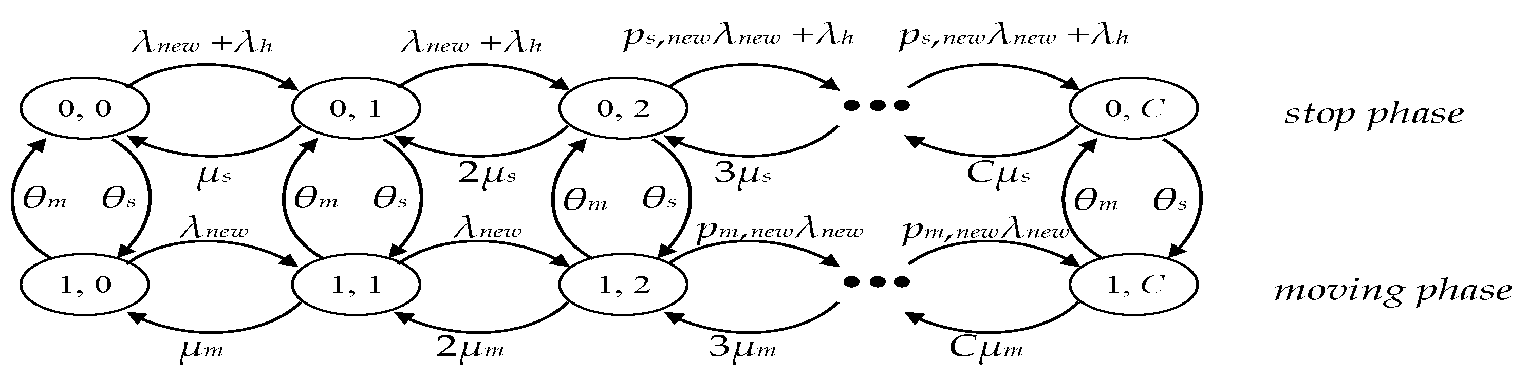
3. The Generalized Probabilistic BR Loss Model

3.1. The Analytical Model

In the generalized probabilistic BR loss model, the probabilistic BR policy is considered in both stop and new phases. More specifically, the CAC mechanism, during the stop phase, is as follows: a handover call is blocked only if all C b.u. are occupied while a new call is blocked: (i) with a predefined probability (1−p_s,new) when the occupied b.u. j = C − t_new, …, C − 1 and (ii) with probability 1 when the occupied b.u. j = C. On the same hand, during the moving phase, a new call is blocked: (i) with a predefined probability (1−p_m,new) when the occupied b.u. j = C − t_new, …, C − 1 and (ii) with probability 1 when the occupied b.u. j = C. Note that if t_new = 0, then p_s,new = p_m,new = 1, i.e., new calls are allowed to have access in all C b.u. in both phases.

Let λ_new and λ_h be the arrival rate for Poisson arriving new and handover calls, respectively. Accepted calls remain in the system for an exponentially distributed service time, with mean ${\mu }_s^{-1}$ in the stop phase and ${\mu }_m^{-1}$ in the moving phase.

The proposed analytical model can be described via the state space diagram of Figure 2, assuming that the reservation space starts in state (0,2). Based on this 2-D Markov chain, let P_g(i,n) be the steady-state probability of the generalized loss model which expresses the fact that the vehicle is in phase i and there exist n users in-service, where $0\le n\le C$.

We initially consider the global balance equations for the boundary states (0,0) and (1,0):

$$\begin{array}{l}\mathrm{state} (0,0): ({\lambda }_{new}+{\lambda }_h+{\theta }_s)P_g(0,0)-{\mu }_s{P}_g(0,1)-{\theta }_m{P}_g(1,0)=0\hspace{1em}\hspace{1em}\hspace{1em}(for i=0,n=0)\\ \mathrm{state} (1,0): ({\lambda }_{new}+{\theta }_m)P_g(1,0)-{\mu }_m{P}_g(1,1)-{\theta }_s{P}_g(0,0)=0\hspace{1em}\hspace{1em}\hspace{1em}\hspace{1em}(fori=1,n=0)\end{array}$$

or in a more compact way:

$$({\lambda }_i(0)+{\theta }_i)P_g(i,0)-{\mu }_i{P}_g(i,1)-{\theta }_j{P}_g(j,0)=0$$

(18)

where ${\lambda }_i(0)=\{\begin{array}{l}{\lambda }_{new}+{\lambda }_h, i=0\\ {\lambda }_{new} , i=1\end{array}, {\theta }_i(0)=\{\begin{array}{l}{\theta }_s , i=0\\ {\theta }_m, i=1\end{array} , {\mu }_i=\{\begin{array}{l}{\mu }_s , i=0\\ {\mu }_m, i=1\end{array} , j=1-i.$

We consider now the states below the system’s capacity, i.e., the states where 0 < n < C. For these states, the following global balance equation can be written:

$$({\lambda }_i(n)+n{\mu }_i+{\theta }_i)P_g(i,n)-{\lambda }_i(n-1)P_g(i,n-1)-{\theta }_j{P}_g(j,n)-(n+1){\mu }_i{P}_g(i,n+1)=0$$

(19)

where ${\lambda }_i(n)=\{\begin{array}{l}{\lambda }_{new}+{\lambda }_h, i=0, 0<n\le C-t_{new}-1\\ p_{s,new}{\lambda }_{new}+{\lambda }_h, i=0, C-t_{new}\le n<C\\ {\lambda }_{new}, i=1, 0<n<C-t_{new}-1\\ p_{m,new}{\lambda }_{new}, i=1, C-t_{new}\le n<C\end{array}, j=1-i.$

Finally, we consider the boundary states (0,C) and (1,C). For these states, we have the following global balance equation:

$$(C{\mu }_i+{\theta }_i)P_g(i,C)-{\lambda }_i(C-1)P_g(i,C-1)-{\theta }_j{P}_g(j,C)=0$$

(20)

To determine the values of P_g(i,n) based on (18)–(20), the iterative algorithm of Section 2.2 can be adopted.

3.2. CBP Determination of New and Handover Calls

The CBP of new calls in the stop phase, $B_{g,s,new}^{}$, can be determined via:

$$B_{g,s,new}^{}=(1-p_{s,new}){\displaystyle \sum _{n=C-t_{new}}^{C-1}{P}_g(0,n)}+P_g(0,C)$$

(21)

In the moving phase of the generalized model, call blocking of new calls occurs not only when there are no available b.u., but also probabilistically in states P_g(1,n) where $C-t_{new}\le n<C$. Consequently, the CBP computation of new calls in the moving phase,$B_{g,m,new}^{}$, is based on the following formula:

$$B_{g,m,new}^{}=(1-p_{m,new}){\displaystyle \sum _{n=C-t_{new}}^{C-1}{P}_g(1,n)}+P_g(1,C)$$

(22)

Based on (21) and (22), the total CBP of new calls, $B_{g,new}^{}$, can be determined via:

$$B_{g,new}^{}=B_{g,s,new}^{}+B_{g,m,new}^{}$$

(23)

The CBP of handover calls in the stop phase, $B_{g,s,h}^{}$, can be determined via:

$$B_{g,s,h}^{}=P_g(0,C)$$

(24)

The CBP of handover calls given stop phase, $B_{g,s,h}^{*}$, can be determined via:

$$B_{g,s,h}^{*}=\frac{B_{g,s,h}^{}}{{\displaystyle \sum _{n=0}^C{P}_g(0,n)}}$$

(25)

Finally, the link utilization, U_g, can be computed via the formula:

$$U_g={\displaystyle \sum _{i=0}^1{\displaystyle \sum _{n=0}^{C}n{P}_g(i,n)}}$$

(26)

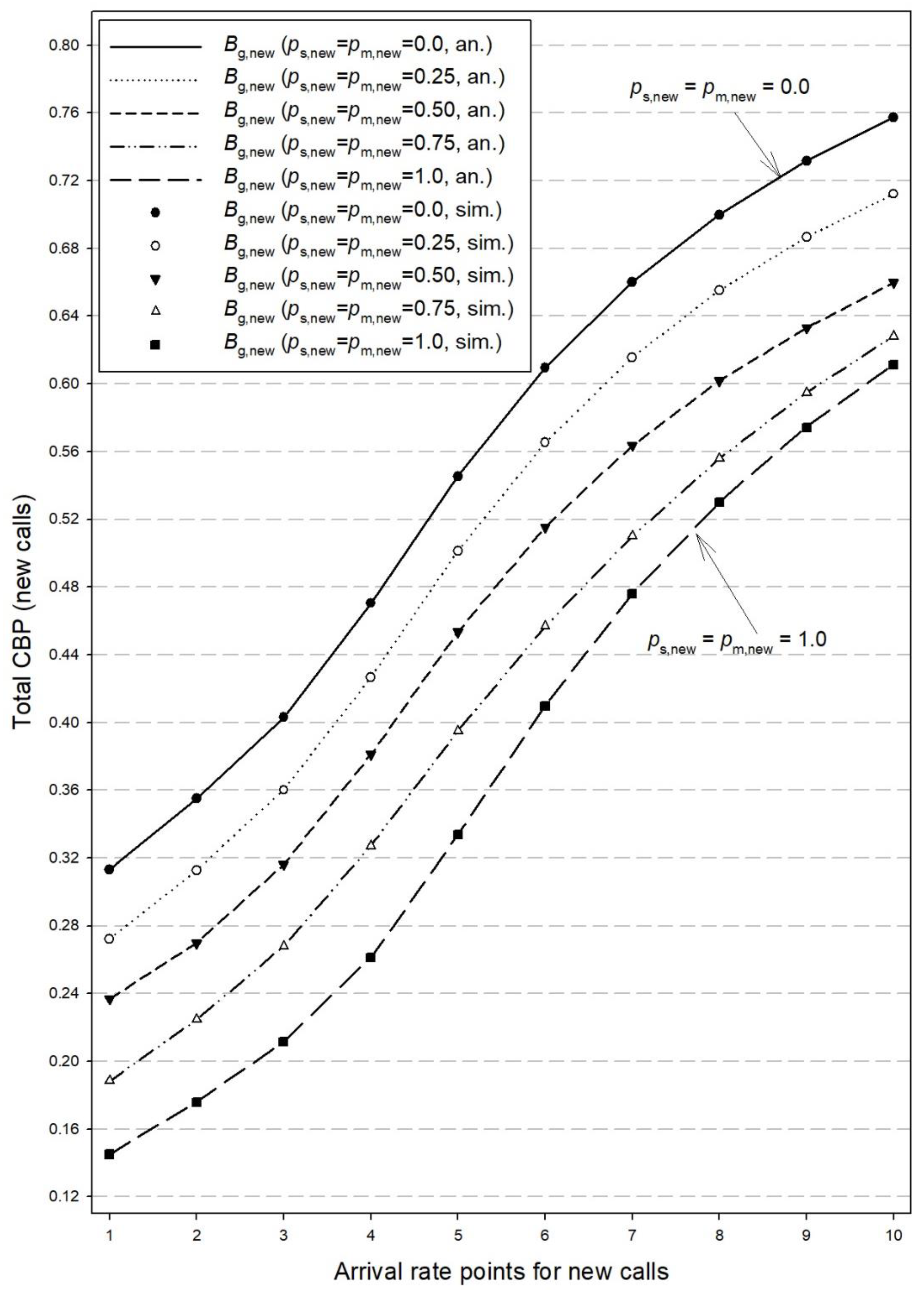
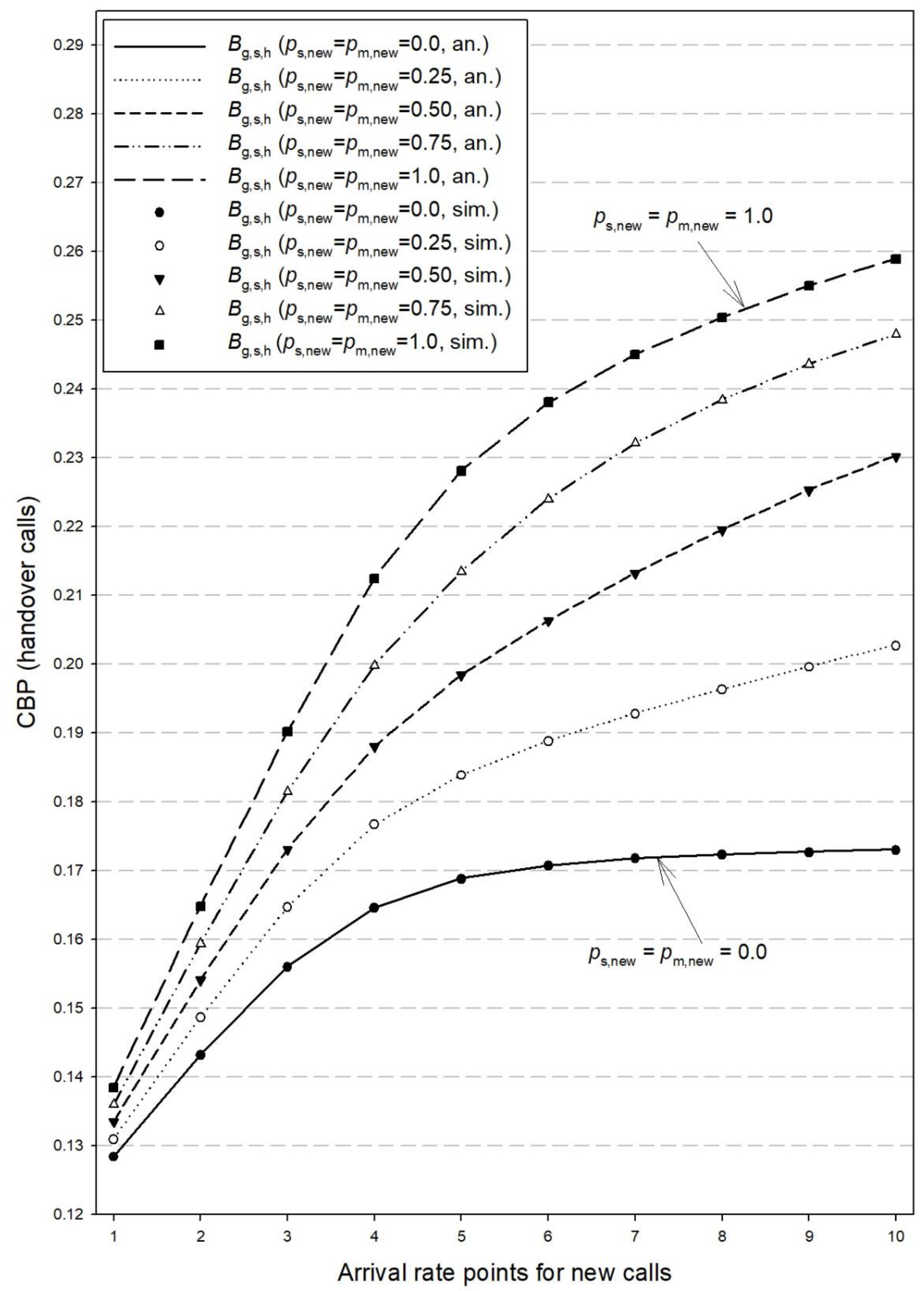
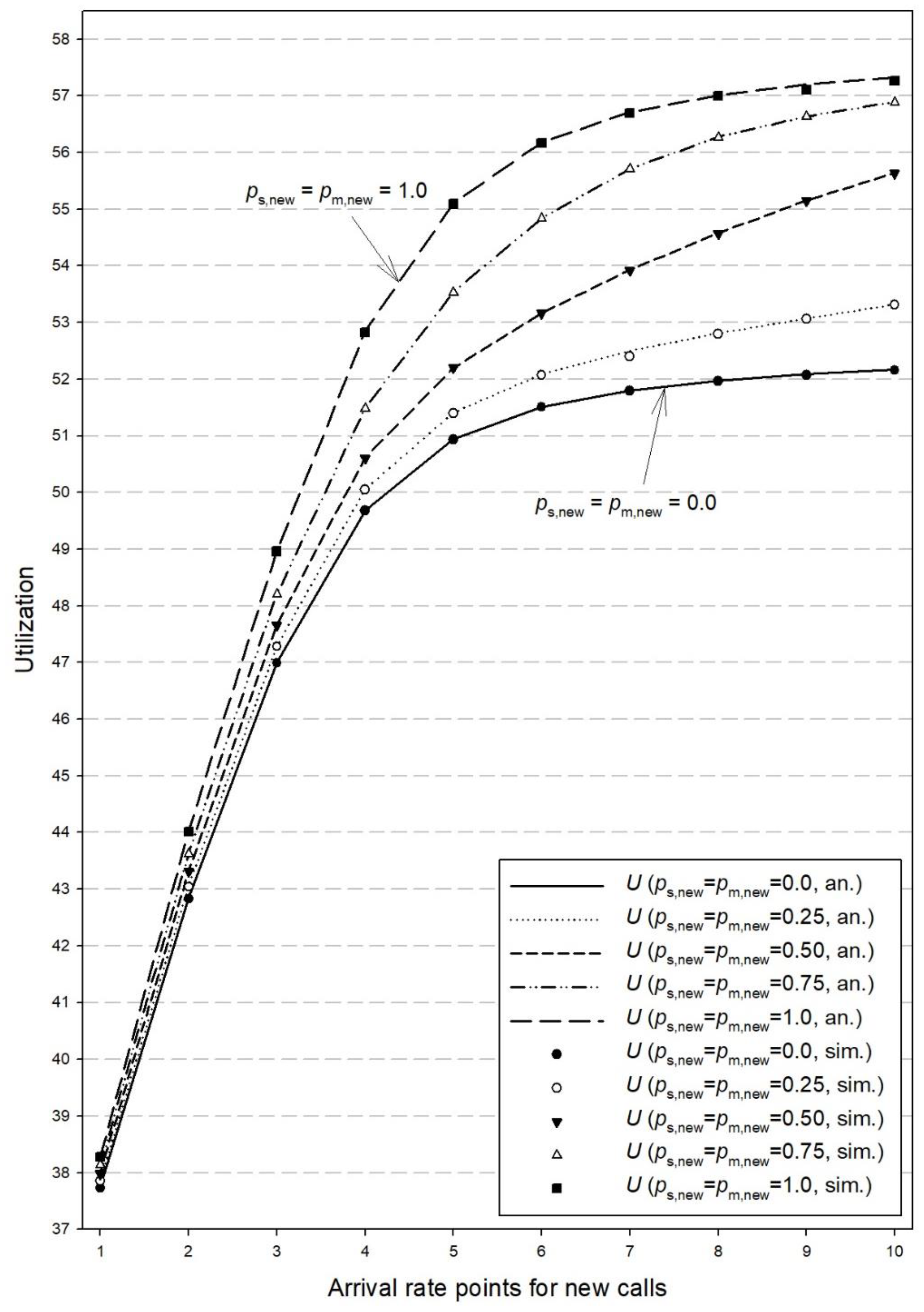
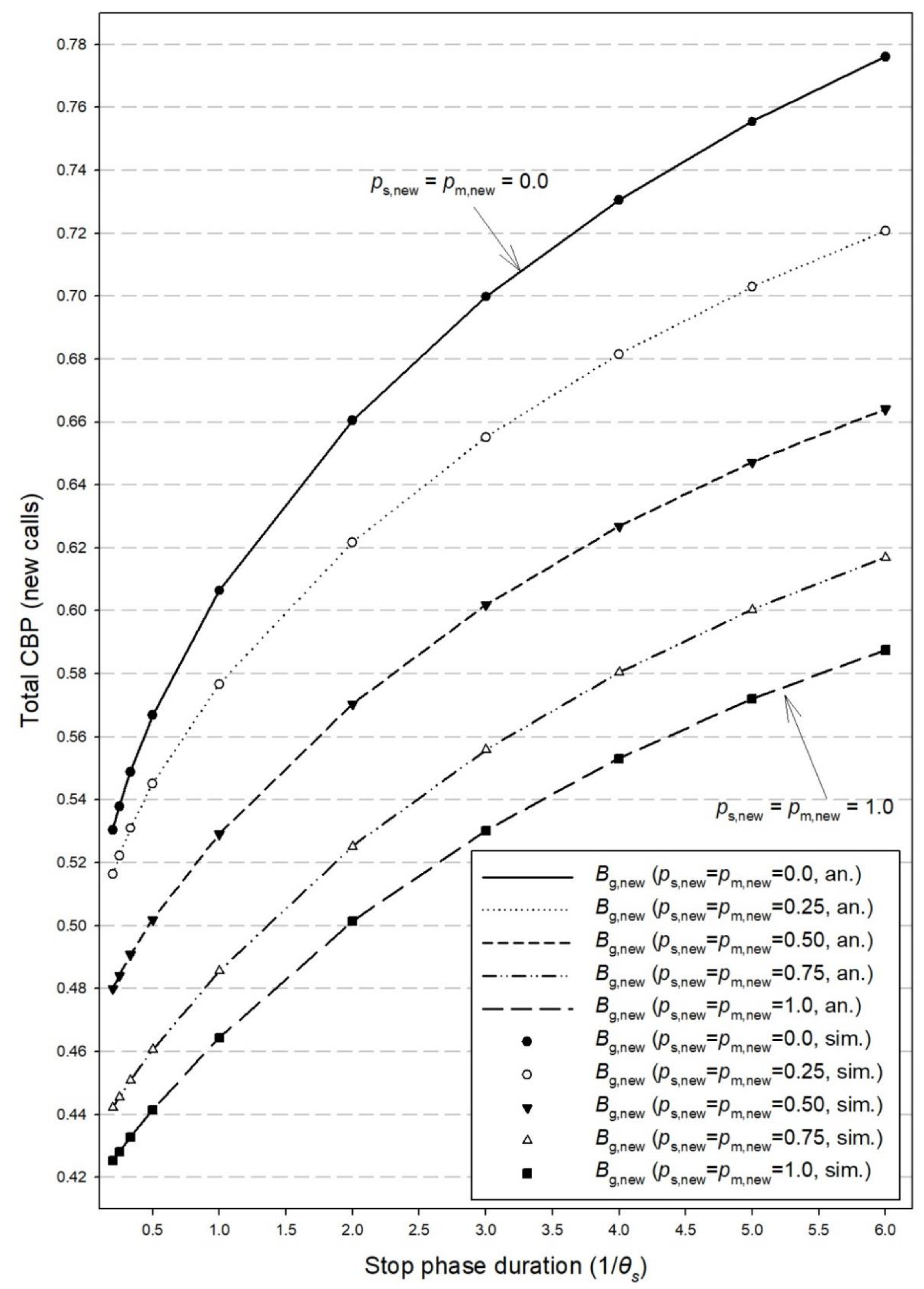
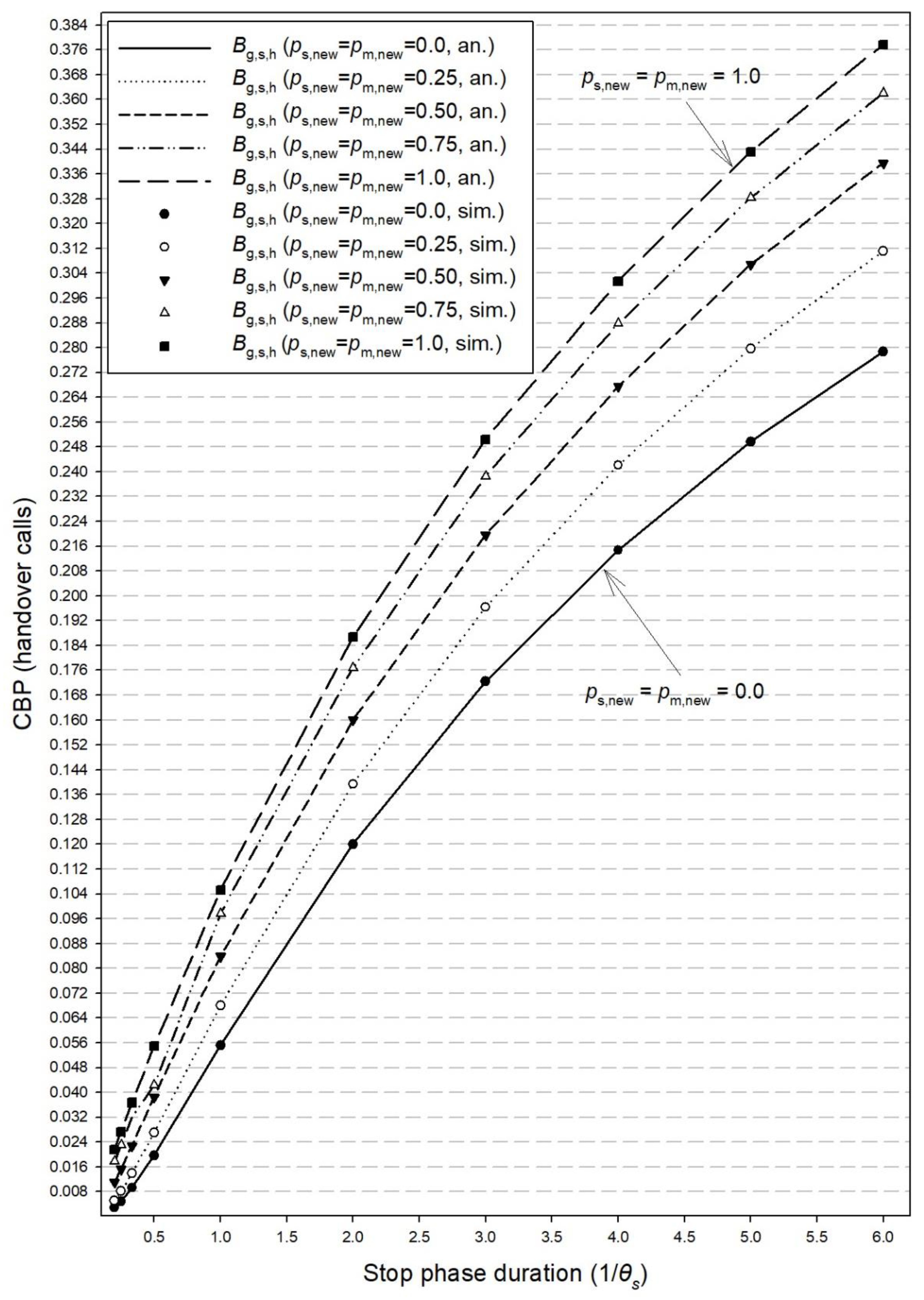
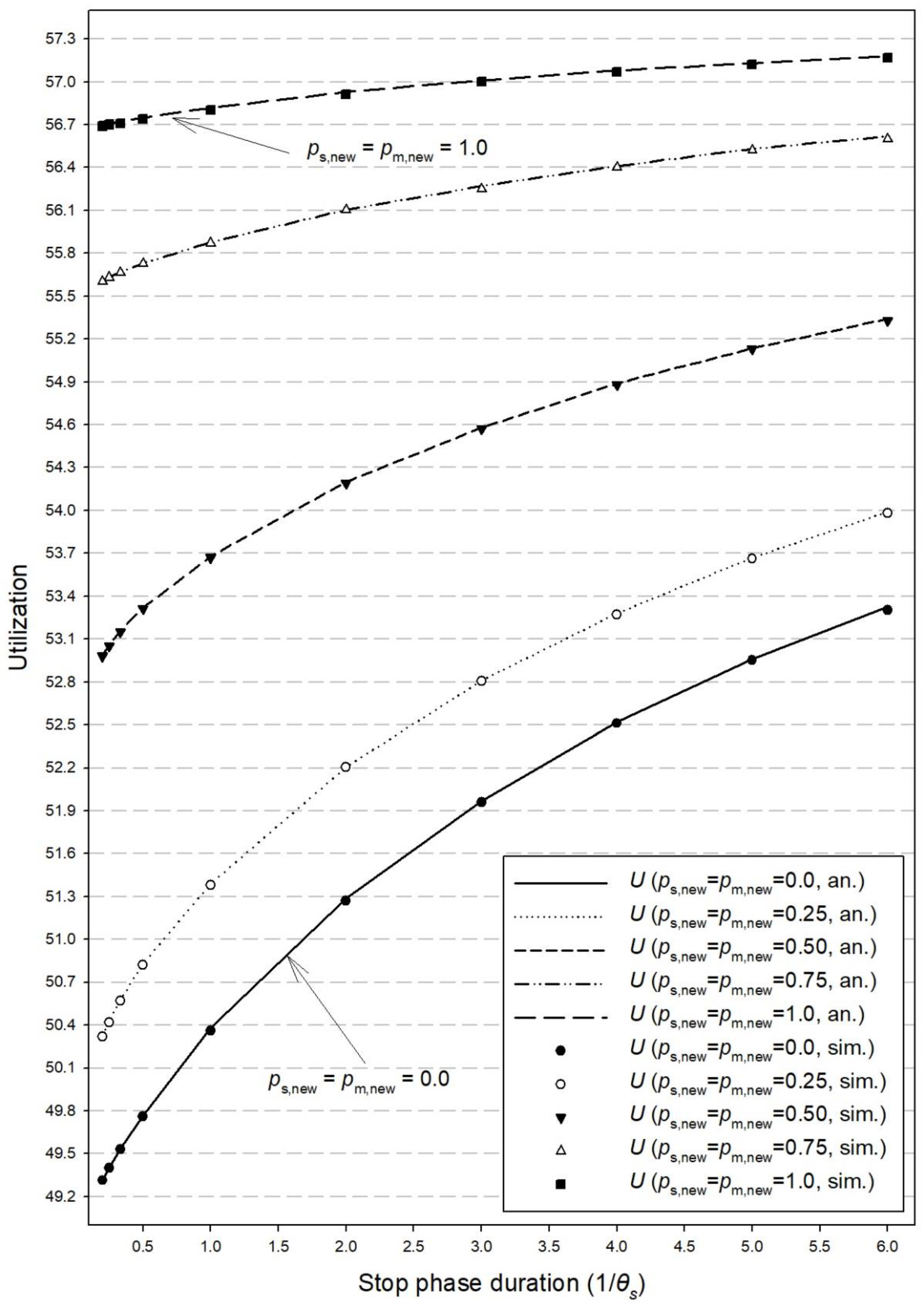
4. Performance Evaluation

In this section, we consider an application example of a vehicle with an AP installed on it and let the capacity of the AP’s WLAN be equal to C = 58 b.u. During the stop phase, the vehicle remains for an exponentially distributed time in a location with mean ${\theta }_s^{-1}$ =3. We also assume that the duration of the moving phase is exponentially distributed with mean ${\theta }_m^{-1}$ = 6. The vehicle accommodates Poisson arriving calls with λ_h = 24 (fixed value) and λ_new = 2 (variable value). Accepted calls remain in the system for an exponentially distributed service time with mean ${\mu }_s^{-1}$ = ${\mu }_m^{-1}$ = 6. To facilitate handover users, the probabilistic BR policy is considered whereby t_new = 8 b.u. are reserved for them. In what follows, the generalized probabilistic BR loss model is considered. To this end, five different sets of p_s,new and p_m,new are considered: (1) p_s,new = p_m,new = 0.0 (this is the cutoff priority scheme studied in [7]); (2) p_s,new = p_m,new = 0.25; (3) p_s,new = p_m,new = 0.50; (4) p_s,new = p_m,new = 0.75; (5) p_s,new = p_m,new = 1.0 (this is the nonpriority scheme studied in [7]). Note that the probabilistic BR loss model refers to the case of p_m,new = 1.0 (the CS policy is applied to new calls and therefore no reservation occurs) and p_s,new < 1.0. Since this model leads to similar conclusions with the generalized loss model, we present analytical and simulation results of the generalized probabilistic BR loss model only. The simulation results presented herein are based on Simscript III and are the mean values of eight runs [25]. In each run, the initial 5% of the generated calls (one million generated calls per run) is not taken into account in the CBP results, in order to obtain a warm-up period [26,27]. Finally, reliability ranges which are less than two orders of magnitude are not presented in the CBP graphs.

Table 1. List of simulation parameters.

AP’s WLAN capacity	C = 58 b.u.
Duration of the stop phase (exponentially distributed)	${\theta }_s^{-1}$ = 3 (mean value)
Duration of the moving phase (exponentially distributed)	${\theta }_m^{-1}$ = 6 (mean value)
Arrival rate of handover calls (Poisson arrivals)	λh = 24 (fixed value)
Arrival rate of new calls (Poisson arrivals)	λnew = 2, 4, 6, 8, 10, 12, 14, 16, 18, 20 (variable value)
Service time in the stop phase (exponentially distributed)	${\mu }_s^{-1}$ = 6 (mean value)
Service time in the moving phase (exponentially distributed)	${\mu }_m^{-1}$ = 6 (mean value)
BR parameter (for new calls)	tnew = 8 b.u.
Probabilistic BR parameters (stop phase)	ps,new = 0.0, 0.25, 0.50, 0.75, 1.0
Probabilistic BR parameters (moving phase)	pm,new = 0.0, 0.25, 0.50, 0.75, 1.0
Number of simulation runs and generated calls/run	Mean values of eight runs with 106 generated calls/run and 5% of them not taken into account (warm-up period)

includes the list of simulation parameters used in this application example.

In the x-axis of Figure 3, Figure 4 and Figure 5, the values of λ_new increase in steps of 2. Thus, point 1 (in the x-axis) refers to λ_new = 2 and point 10 refers to λ_new = 20. In the x-axis of Figure 6, Figure 7 and Figure 8, we consider 10 different values of ${\theta }_s^{-1}$, assuming that λ_h = 24 (fixed value), λ_new = 16 (fixed value) and ${\theta }_m^{-1}$ = 6 (fixed value). More precisely, we consider the values 0.2, 0.25, 0.3333, 0.5, 1.0, 2.0, 3.0, 4.0, 5.0 and 6.0. To increase the readability of all graphs, simulation results are represented with different types of dots, while analytical results are represented with different types of lines. Besides, two different arrows have been included in each graph in order to identify the results obtained via [7]. An arrow identifies the case of p_s,new = p_m,new = 0.0 (the cutoff priority scheme of [7]) and another arrow identifies the case of p_s,new = p_m,new = 1.0 (the nonpriority scheme of [7]).

Figure 3 presents the analytical together with the simulation results of the total CBP of new calls for the five different sets of p_s,new and p_m,new. Figure 4 presents the corresponding results of the CBP of handover calls (based on (15) and (24)). Finally, Figure 5 presents the analytical and simulation results of the system’s utilization. All graphs show that the analytical results are similar to the corresponding simulation results. Regarding Figure 3, we observe that: (i) the increase of λ_new increases the total CBP of new calls; (ii) the choice of p_s,new and p_m,new affects the CBP, leading to high CBP values (when p_s,new = p_m,new = 0.0) and low CBP values (when p_s,new = p_m,new = 1.0); (iii) the CBP results obtained via [7] cannot capture the behavior of the proposed models, a fact that is expected since the models of [7] do not consider the case of the probabilistic BR policy. Regarding Figure 4, we observe that: (i) the increase of λ_new increases the CBP of handover calls (in the stop phase); (ii) the choice of p_s,new and p_m,new affects the CBP of handover calls leading to high CBP values (when p_s,new = p_m,new = 1.0) and low CBP values (when p_s,new = p_m,new = 0.0) (i.e., the increase of p_s,new and p_m,new has the opposite impact on the CBP of new and handover calls); (iii) the CBP results obtained via [7] cannot capture the behavior of the proposed models. Finally, regarding Figure 5, we observe that: (i) the increase of λ_new increases the system’s utilization and (ii) a slightly higher utilization appears when p_s,new = p_m,new = 1.0 (i.e., when the BR policy is not applied in favor of handover calls).

In Figure 6, Figure 7 and Figure 8, we present the total CBP of new calls (Figure 6), the CBP of handover calls in the stop phase (Figure 7) and the system’s utilization (Figure 8) for the different values of ${\theta }_s^{-1}$. Our conclusions are similar to those obtained in Figure 3, Figure 4 and Figure 5. In addition, we observe that an increase of ${\theta }_s^{-1}$ results in the CBP increase of both types of calls. This is expected, since the increase of the stop phase duration results in increased new and handover calls competing for acceptance in the system.

5. Conclusions

We propose two loss models for a mobile hotspot that accommodates new and handover users. To favor handover users but at the same time not substantially increase the CBP of new users, we propose the probabilistic BR policy where new calls may enter the reservation space with a certain, predefined, probability. In the first loss model, the probabilistic BR policy is applied only to new calls during the stop phase of a vehicle. In the second loss model, a generalization is considered, where the probabilistic BR policy can be applied not only during the stop phase but also during the moving phase. Both models are analytically described with the aid of two-dimensional Markov chains, while iterative algorithms are proposed for the determination of the steady-state probabilities and the various performance measures such as CBP and system’s utilization.

As a future study, we will extend these models to include the case of quasi-random traffic, where a finite number of users may generate calls in the system not only during the stop but also during the moving phase. Additionally, we intend to study the case of multiservice traffic where users generate traffic (either random or quasi-random) and have different bandwidth-per-call requirements, i.e., a user may request more than a single b.u. in order to be accepted in the system. Such extensions have been considered in the literature in wired/wireless networks but not in the case of mobile hotspots [28,29,30,31,32,33,34,35,36].

References

1. Halabian, H.; Rengaraju, P.; Lung, C.-H.; Lambadaris, I. A reservation-based call admission control scheme and system modeling in 4G vehicular networks. EURASIP J. Wirel. Commun. Netw. 2015, 2015, 125. [Google Scholar] [CrossRef] [Green Version]
2. Głąbowski, M.; Kaliszan, A.; Stasiak, M. Modelling overflow systems with distributed secondary resources. Comput. Netw. 2016, 108, 171–183. [Google Scholar] [CrossRef]
3. Chousainov, I.-A.; Moscholios, I.; Kaloxylos, A.; Logothetis, M. Performance Evaluation in Single or Multi-Cluster C-RAN Supporting Quasi-Random Traffic. J. Commun. Softw. Syst. 2020, 16, 170–179. [Google Scholar] [CrossRef]
4. Chousainov, I.-A.; Moscholios, I.; Sarigiannidis, P.; Kaloxylos, A.; Logothetis, M. An analytical framework of a C-RAN sup-porting random, quasi-random and bursty traffic. Comput. Netw. 2020, 180, 107410. [Google Scholar] [CrossRef]
5. Vazquez-Avila, J.; Cruz-Perez, F.; Ortigoza-Guerrero, L. Performance analysis of fractional guard channel policies in mobile cellular networks. IEEE Trans. Wirel. Commun. 2006, 5, 301–305. [Google Scholar] [CrossRef]
6. Kim, Y.; Pack, S.; Lee, W. Mobility-Aware Call Admission Control Algorithm in Vehicular WiFi Networks. In Proceedings of the 2010 IEEE Global Telecommunications Conference, Miami, FL, USA, 6–10 December 2010. [Google Scholar]
7. Kim, Y.; Ko, H.; Pack, S.; Lee, W.; Shen, X. Mobility-Aware Call Admission Control Algorithm with Handoff Queue in Mobile Hotspots. IEEE Trans. Veh. Technol. 2013, 62, 3903–3912. [Google Scholar] [CrossRef] [Green Version]
8. Kim, C.; Klimenok, V.; Dudin, A. Analysis and optimization of Guard Channel Policy in cellular mobile networks with account of retrials. Comput. Oper. Res. 2014, 43, 181–190. [Google Scholar] [CrossRef]
9. Moscholios, I.D.; Vassilakis, V.G.; Logothetis, M.D.; Boucouvalas, A.C. State-Dependent Bandwidth Sharing Policies for Wireless Multirate Loss Networks. IEEE Trans. Wirel. Commun. 2017, 16, 5481–5497. [Google Scholar] [CrossRef] [Green Version]
10. Omheni, N.; Gharsallah, A.; Zarai, F. An enhanced radio resource management based MIH policies in heterogeneous wireless networks. Telecommun. Syst. 2017, 67, 577–592. [Google Scholar] [CrossRef]
11. Panagoulias, P.I.; Moscholios, I.D. Congestion probabilities in the X2 link of LTE networks. Telecommun. Syst. 2019, 71, 585–599. [Google Scholar] [CrossRef]
12. Efstratiou, P.; Moscholios, I. User Mobility in a 5G Cell with Quasi-Random Traffic under the Complete Sharing and Bandwidth Reservation Policies. Autom. Control. Comput. Sci. 2019, 53, 376–386. [Google Scholar] [CrossRef]
13. Lee, D.-S.; Hsueh, Y.-H. Bandwidth-Reservation Scheme Based on Road Information for Next-Generation Cellular Networks. IEEE Trans. Veh. Technol. 2004, 53, 243–252. [Google Scholar] [CrossRef]
14. Pati, H.K. A control-period-based distributed adaptive guard channel reservation scheme for cellular networks. Wirel. Netw. 2013, 19, 1739–1753. [Google Scholar] [CrossRef]
15. Nadembega, A.; Hafid, A.; Taleb, T. Mobility Prediction-aware Bandwidth Reservation Scheme for Mobile Networks. IEEE Trans. Veh. Technol. 2014, 64, 2561–2576. [Google Scholar] [CrossRef]
16. Moscholios, I.D.; Logothetis, M.D.; Vardakas, J.S.; Boucouvalas, A.C. Performance metrics of a multirate resource sharing teletraffic model with finite sources under the threshold and bandwidth reservation policies. IET Netw. 2015, 4, 195–208. [Google Scholar] [CrossRef]
17. Keramidi, I.; Moscholios, I.; Sarigiannidis, P.; Logothetis, M. Blocking Probabilities in a Mobility-Aware CAC Algorithm of a Vehicular WiFi Network. In Proceedings of the 2021 IEEE Microwave Theory and Techniques in Wireless Communications (MTTW), Riga, Latvia, 7–8 October 2021. [Google Scholar]
18. Stasiak, M.; Głąbowski, M.; Wisniewski, A.; Zwierzykowski, P. Modeling and Dimensioning of Mobile Networks: From GSM to LTE; John Wiley: Hoboken, NJ, USA, 2011. [Google Scholar]
19. Logothetis, M.; Moscholios, I.D. Efficient Multirate Teletraffic Loss Models Beyond Erlang; John Wiley & IEEE Press: Hoboken, NJ, USA, 2019. [Google Scholar]
20. Xu, Q.; Ji, H.; Li, X.; Zhang, H. Admission Control Scheme for Service Dropping Performance Improvement in High-Speed Railway Communication Systems. IEEE Trans. Veh. Technol. 2015, 65, 5251–5263. [Google Scholar] [CrossRef]
21. Sun, N.; Zhao, Y.; Sun, L.; Wu, Q. Distributed and Dynamic Resource Management for Wireless Service Delivery to High-Speed Trains. IEEE Access 2017, 5, 620–632. [Google Scholar] [CrossRef]
22. Kim, S. Bargaining-Based Spectrum Allocation Algorithm for High-Speed Railway Communications. IEEE Access 2021, 9, 71651–71659. [Google Scholar] [CrossRef]
23. Huang, Q.; Ko, K.-T.; Iversen, V. Approximation of loss calculation for hierarchical networks with multiservice overflows. IEEE Trans. Commun. 2008, 56, 466–473. [Google Scholar] [CrossRef]
24. Hanczewski, S.; Stasiak, M.; Zwierzykowski, P. Modelling of the access part of a multi-service mobile network with service priorities. EURASIP J. Wirel. Commun. Netw. 2015, 2015, 194. [Google Scholar] [CrossRef] [Green Version]
25. Rice, S.; Marjanski, A.; Markowitz, H.; Bailey, S. The SIMSCRIPT III programming language for modular object-oriented sim-ulation. In Proceedings of the Winter Simulation Conference, Orlando, FL, USA, 4 December 2005. [Google Scholar]
26. Jain, R. The Art of Computer Systems Performance Analysis; John Wiley & Sons: Hoboken, NJ, USA, 1991. [Google Scholar]
27. Robinson, S. A statistical process control approach to selecting a warm-up period for a discrete-event simulation. Eur. J. Oper. Res. 2007, 176, 332–346. [Google Scholar] [CrossRef]
28. Kaufman, J. Blocking in a Shared Resource Environment. IEEE Trans. Commun. 1981, 29, 1474–1481. [Google Scholar] [CrossRef]
29. Roberts, J. A service system with heterogeneous user requirements. In Performance of Data Communications Systems and Their Applications; Elsevier: Amsterdam, The Netherlands, 1981; pp. 423–431. [Google Scholar]
30. Głąbowski, M.; Stasiak, M. Point-to-point blocking probability in switching networks with reservation. Ann. Telecommun. 2002, 57, 798–831. [Google Scholar]
31. Moscholios, I.D.; Logothetis, M.D.; Nikolaropoulos, P.I. Engset multi-rate state-dependent loss models. Perform. Eval. 2005, 59, 247–277. [Google Scholar] [CrossRef]
32. Vassilakis, V.G.; Moscholios, I.D.; Logothetis, M.D. The extended connection-dependent threshold model for call-level performance analysis of multi-rate loss systems under the bandwidth reservation policy. Int. J. Commun. Syst. 2012, 25, 849–873. [Google Scholar] [CrossRef]
33. Parniewicz, D.; Stasiak, M.; Zwierzykowski, P. Traffic Engineering for Multicast Connections in Multiservice Cellular Networks. IEEE Trans. Ind. Inform. 2012, 9, 262–270. [Google Scholar] [CrossRef]
34. Moscholios, I.; Logothetis, M.; Shioda, S. Performance Evaluation of Multirate Loss Systems Supporting Cooperative Users with a Probabilistic Behavior. IEICE Trans. Commun. 2017, E100.B, 1778–1788. [Google Scholar] [CrossRef]
35. Nowak, B.; Piechowiak, M.; Stasiak, M.; Zwierzykowski, P. An analytical model of a system with priorities servicing a mixture of different elastic traffic streams. Bull. Pol. Acad. Sci. Tech. Sci. 2020, 68, 263–270. [Google Scholar]
36. Hanczewski, S.; Stasiak, M.; Weissenberg, J. A Model of a System with Stream and Elastic Traffic. IEEE Access 2021, 9, 7789–7796. [Google Scholar] [CrossRef]
Figure 1. The 2-D state transition diagram in the proposed probabilistic BR loss model.
Telecom 02 00031 g001
Figure 2. The 2-D state transition diagram in the proposed generalized probabilistic BR loss model.
Telecom 02 00031 g002
Figure 3. Total CBP of new calls for different values of λnew.
Telecom 02 00031 g003
Figure 4. CBP of handover calls (in the stop phase) for different values of λnew.
Telecom 02 00031 g004
Figure 5. Utilization for different values of λnew.
Telecom 02 00031 g005
Figure 6. Total CBP of new calls for different values of θ s 1
Telecom 02 00031 g006
Figure 7. CBP of handover calls (in the stop phase) for different values of θ s 1 .
Telecom 02 00031 g007
Figure 8. Utilization for different values of θ s 1 .
Telecom 02 00031 g008