1. Introduction
Vehicles powered by an internal combustion engine are now the main means of transport for both passenger and freight. Due to more than 100 years of development and improvement, they have achieved a considerable degree of excellence. Many types of internal combustion engines have been developed. However, they are not without drawbacks. One of these drawbacks is relatively low efficiency of converting the energy contained in the fuel into useful mechanical energy for propulsion. Much of the energy in the fuel is lost as the engine heat. The other one is the emission of carbon dioxide and other components of the exhaust gas.
Carbon dioxide, although harmless to living organisms, is considered one of the main causes of climate warming. On the other hand, the exhaust contains some number of small particles of solid, liquid, and gaseous substances [
1] forming an aerosol with the air, so-called “smog”. This makes breathing difficult, and some of the individual substances contained in it can cause various diseases or lead to poisoning. The content of emitted substances in exhaust gases depends on several factors determined by the engine design in one side, and style of driving on the other. This issue was discussed in several publications, e.g., [
2], and is reviewed in the paper [
3].
Intensive research aimed at reducing the negative impact on the atmosphere is conducted in many centers around the world [
4]. The conclusions indicate such directions of development as developing technologies of alternative energy sources, including alternative fuels, introducing electric or hybrid vehicles and modernizing of the vehicle structure. [
5,
6,
7]. The use of biodiesel in public transport was recently studied in [
8]. The energetic efficiency of biofuel production, defined as the ratio of the energy delivered by the system to the sum of energy inputs needed to perform all processes necessary to obtain and deliver the above-mentioned amount of energy, was discussed in several papers of the present author and collaborators, and summarized in the book [
9]. These works indicate that the contribution of energy needed to produce biofuels is relatively high as compared to the energy obtained in the form of biofuel. Therefore, biofuel production involves substantial amount of land to be used for energetic plantations competing with food crops. As a remedy for this competition the use of various organic wastes as well as marine algae is proposed. Another approach to alternative means of powering vehicles is to use hydrogen through direct combustion in the engine [
10], or to use an electric motor powered by electricity from a hydrogen fuel cell [
11,
12]. Hydrogen is also proposed as fuel in other than road types of transportation [
13]. Several works are also devoted to the requirements to be met to use hydrogen fuel in practice. This mainly concerns the need for necessary infrastructure [
14]. The paper [
15], in turn, proposes the modern design of automobile that would assure very high performance of the construction combined with hydrogen fuel cell.
The other solution for transport is the use of electricity for vehicle’s powering. Comparison of the electromobility development in several countries and its effect on CO
2 emission mitigation was also recently given in Swic at al. [
16]. Actually, many papers are published dealing with various aspects of electromobility. The technology of the electric vehicles has already achieved several variants of technical design [
17]. The main types of electric vehicles are the two variants of hybrid cars that use an internal combustion engine together with an electric motor. In one of the solutions, the electric motor works with a battery being charged while the internal combustion engine is running (HEV), in the other, the battery is additionally charged with a charger connected to the electric grid (PHEV). A certain amount of electricity is recovered while the vehicle is slowing down. There are also vehicles (type BEV) that are only equipped with an electric motor and a battery charged from the grid [
18]. In several publications, the issues of limitations related to both the design of the vehicle drive system and its charging from the electrical network are considered [
19,
20,
21]. Several papers also discuss the shift of carbon dioxide emissions from the road to electric power stations due to electricity consumed by electric vehicles charged from the grid [
22,
23]. Experimental studies on exhaust composition and energy consumption for various types of vehicles were performed, and compared to those of internal combustion engine [
24]. The results clearly show the lower energy consumption and lower emissions of vehicles equipped with an electric driveline component.
Several works are dedicated to the problems related to the popularization of an increase of the share of electric vehicles among the vehicles used [
25,
26,
27,
28].
An attempt to modeling the diffusion of new transportation means is presented in paper [
29] predicting the dominance of fuel cell electric vehicles after a long time and will be preceded by hybrid vehicles. In fact, this trend is already observed in everyday life. The game theory is applied in the work [
30] to analyze market dynamics and criteria affecting behavior of consumers purchasing electric cars, and investors building charging stations.
The interactions between electric vehicles and the smart grid are analyzed in the work [
31] showing that the optimization and stabilization of the grid can be achieved through intelligent way of charging the vehicles.
The papers [
32,
33] present results of forecasting the development of electromobility in Poland, and its effects on power system. Both papers (similar to cited earlier [
23]) use the logistic function of the form:
where
a is s.c. carrying capacity describing the saturation value of the function
y(
t),
t is time, while
b and
c are the parameters determining position and detailed shape of the function. Such function of sigmoidal shape is frequently used [
34,
35,
36] for description or analysis of many processes that reach asymptotic value at
a. The logistic function is used in many modified variants. It must be noted, however, that this simple version presented in Equation (1) describes the transition in which something is created and lasts for the rest of time being of interest. Consequently, in the cases when the product formed at some instant of time may disappear at another instant of time the function should be modified.
In the works cited above, two logistic functions were introduced, one of which described changes in the number of classic cars, and the other the share of electric cars. The parameters of both functions were determined based on the existing actual data.
The aim of the present work is to formulate more elastic logistic model that would describe progress of production of new category of vehicles (e.g., electric ones) that replace old category of vehicles (e.g., with internal combustion engines), and therefore would enable predicting of the consequences of such replacement. The model should allow for such a selection of parameters to create different variants of the course of changes in the number of vehicles in both categories and the related impact on the demand for energy (fuel) and the impact on the natural environment.
2. Materials and Methods
The model proposed in the present work is based on the following assumptions:
- (1)
The production process of vehicle generation can be described by means of a logistic function.
- (2)
The process of decommissioning vehicles of the same generation can also be described by a logistic function shifted in time from the production function.
- (3)
Parameters characterizing the shape of the curve (M and B) may be different for both functions.
- (4)
The actual number of vehicles in use is the difference between the cumulative numbers of vehicles produced till a given instant of time and that of recalled during the same time.
- (5)
The production process of the new generation (e.g., electric) may be coordinated in time with the recall of old generation waste vehicles or it may be delayed or ahead of it.
- (6)
The process of decommissioning of new generation vehicles is correspondingly delayed as compared to the production of this generation.
The corresponding mathematical expression is given as Equation (2).
where
N(
t) is the cumulative number of vehicles existing in time
t,
K is carrying capacity, what means the maximum (asymptotic) number of vehicles,
N0 is an initial number of vehicles (assumed to avoid negative values in the initial run of the function).
Bb [1/year] is a parameter defining the average rate of the production process, and
Mb [year] is the position of the curve of time scale, while
Bd [1/year] and
Md [year] denote corresponding parameters for the scrapping process,
t [year] is time.
In the numerical part of the work the dependencies of
N(
t) are used to compute fuel consumption, expressed in form of energy consumption and carbon dioxide emission. The heating value for fossil fuel is assumed 32 MJ/dm
3, and for computation of CO
2 emission the following values for gasoline were adapted: 69.3 kgCO
2/GJ or 0.25 kgCO
2/kWh [
37].
For the case of emission from electric power stations two values were taken into account: the minimal in EU equal 0.013 kgCO
2/kWh, and maximal 0.819 kgCO
2/kWh [
38,
39].
The energy,
Eg(
t), consumed by
Ng(
t) of gasoline powered vehicles is computed as:
where:
D [km] is the assumed average distance driven by particular class of vehicles,
Q [MJ/dm3] is the lower heating value of the fuel
F [dm3/km] is the assumed value of the specific fuel consumption for a given class of vehicles
k = 2.78·10−7 conversion factor [MJ/GWh]
The energy,
Ee(
t), consumed by
Ne(
t) electric vehicles, in turn, is computed according to Equation (4):
where:
φ [GWh/km] is the assumed value of a specific energy consumption for a given class of electric vehicles.
The initial data for numerical computation for gasoline powered vehicles, as well as for three sets of initial data concerning electric vehicles, from which the first precedes, the second is delayed, and the third is coordinated with the process for gasoline powered cars, are presented in
Table 1.
The values of B [1/year] are assumed arbitrary, but assure that the average rate of manufacturing is higher than average rate of scrapping. Values of M [year] decide about positions of curves on time scale. The variants for electric cars are chosen such that for the first manufacturing curve precedes the scrapping curve of gasoline powered cars, in second they practically overlap, while in the third variant occurs after the curve for scrapping gasoline powered vehicles. The parameter values are deliberately selected in such a way as to obtain the assumed course of both functions
Preliminary computations were performed with the use of MS Excel, and finally the work was done using Microcal OriginPro 2020b. (OriginLab Corporation, One Roundhouse Plaza, Suite 303, Northampton, MA 01060, USA).
3. Results
The values given in
Table 1 are purely theoretical, although the effort was made to keep them as close as possible to realistic values.
Results of numerical computations are presented in subsections of this paper. In spite that computations were performed for various values of annual car mileage or specific fuel consumption, but presented results are confined to 10,000 km/an., and only some values of either specific fuel consumption or electric energy consumption. Those values might have big effect on absolute values of results in a global scale, but do not affect the character of relations published in the paper since the changes of the individual characteristics lead to proportional changes in the final results. The real fuel consumption of the vehicle depends on many factors such as engine capacity, velocity of movement, type of road, etc. [
40] Assumption of numerical values of such characteristics as specific fuel consumption can be considered to be corresponding to some, individual category of the vehicles, and to the average over long time of use of the vehicle. Additionally, computations are made taking into account only the energy consumed by populations of vehicles. On this stage of work the loses of energy in electric grid, as well as energy needed to provide a fuel to internal ignition fossil fuel cars or hydrogen fueled vehicles is not taken into account. These problems will be estimated in further research.
3.1. Number of Vehicles in Use
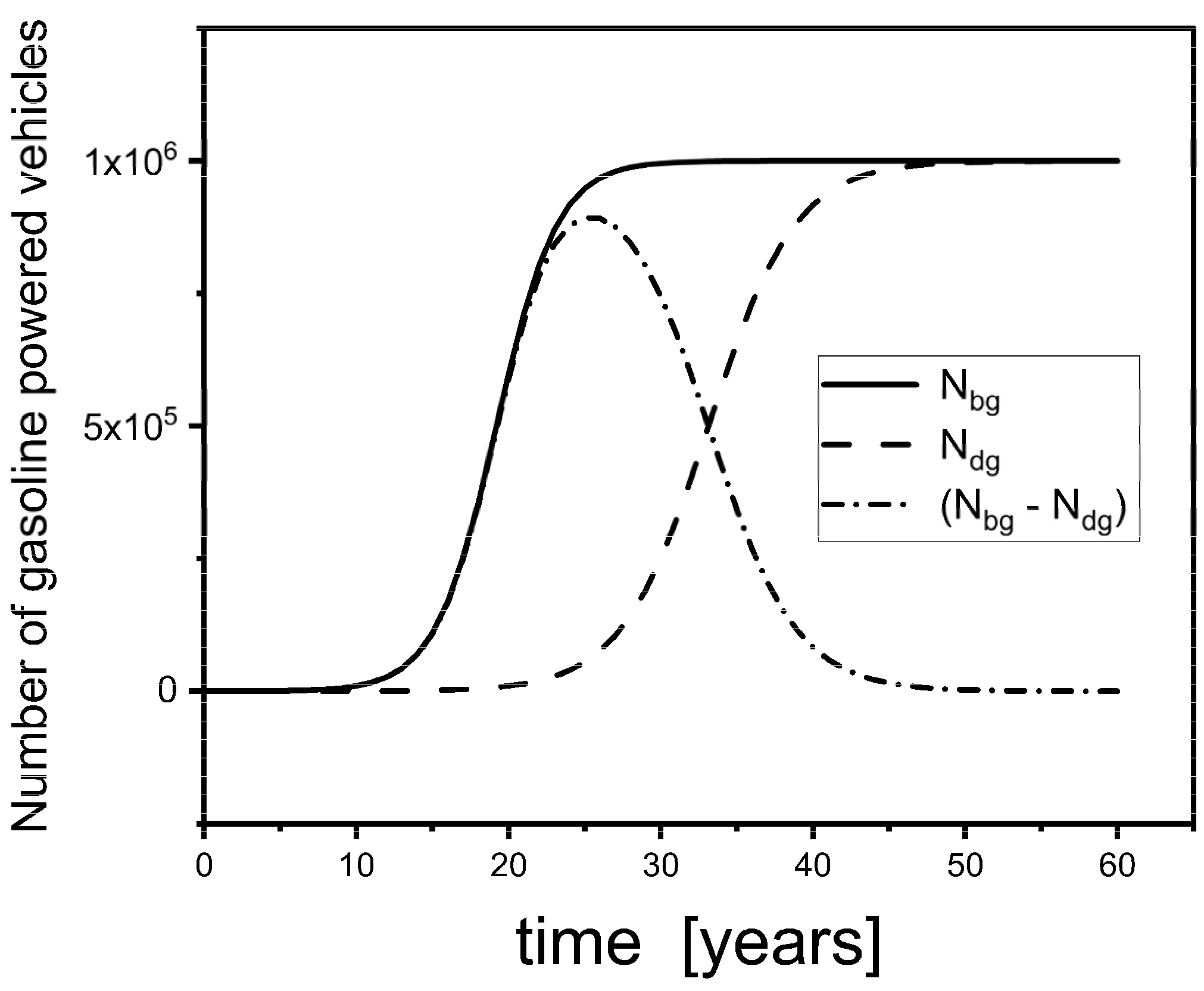
The shapes of functions describing production and scrapping processes for gasoline powered vehicles (computed based on the data in first two columns in
Table 1) as well as their difference are shown in
Figure 1. It is clearly visible that both: production and scrapping curves exhibit typical sigmoidal shape, they are shifted one with respect to the other due to differences in parameter
M, and have different slopes of the middle, rising part of each curve (due to the differences in parameter
B). The difference between them is a bell-shaped curve which overlap with the production curve at the beginning, and after reaching maximum decreases to null at longer times. As mentioned earlier, this curve shows the cumulative number of vehicles still in use.
The electric vehicles are discussed using three variants the first one, computed with M = 5 shows an increase of the plot earlier than the function for gasoline powered vehicle. In the second, the production curve exactly corresponds to production curve for gasoline powered car, and the third—the most interesting—the production curve is computed with the value M = 20, the same as decommissioning curve for internal ignition vehicle. It means that this variant is designed to replace the scrapped gasoline fueled vehicles.
The curves mentioned above, are shown in
Figure 2a.
Figure 2b shows the cumulative distribution functions for all three variants of electric vehicle production. The curves are practically identical, only being shifted on the time scale. It can be seen that the function describing distribution for the first variant of electric vehicle appears earlier than the function for gasoline fueled internal combustion engine. The third function is, in turn, shifted to later period of time.
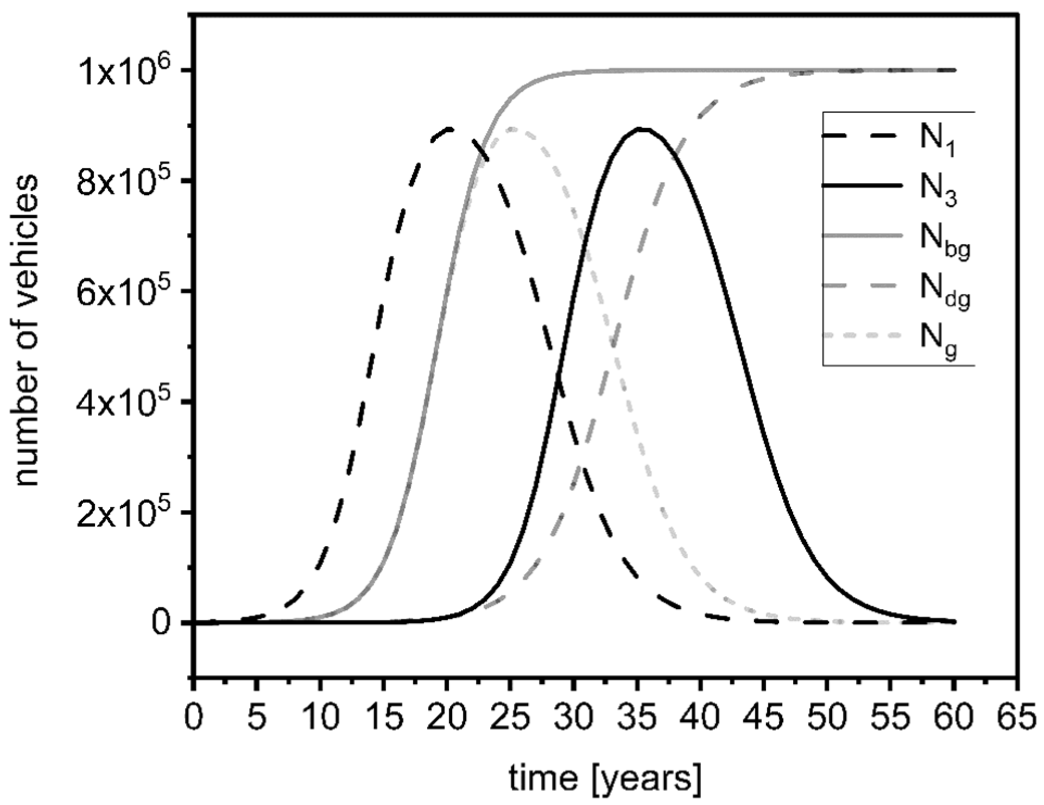
In
Figure 3, time-dependent distribution functions for variants 1, and 3 of electric vehicles are superimposed on the production and decommissioning functions for vehicles equipped with gasoline engine.
It is seen that important part of the distribution function for the first variant precedes the development of the production. In reality such situation seems to be impossible when the new product is created to replace the old technology. It is, however, quite possible when two categories of the product are developed simultaneously. The distribution for the third variant slightly precedes the decommissioning function of traditional vehicles. It is the consequence of the assumption that the production process is assumed to occur faster than the decommissioning i.e., Bb3 > Bdg. It means that even in this case temporarily total number of vehicles (classical and electric) in some period of time increases due to coexistence of both types. It also makes the chance that even slight delay of the production function for electric vehicles may in short time compensate for disappearing classical ones.
3.2. Energy Consumption
The fuel consumption by classical internal combustion engine cars can be expressed in terms of energy consumed. Such presentation enables easier comparison with energy consumption of electric vehicles. Taking into account that time distributions of the number of different types of vehicles discussed above are very similar or just identical one might expect that fuel energy consumption for variants discussed may differ only if values of specific fuel consumption of individual cars differ.
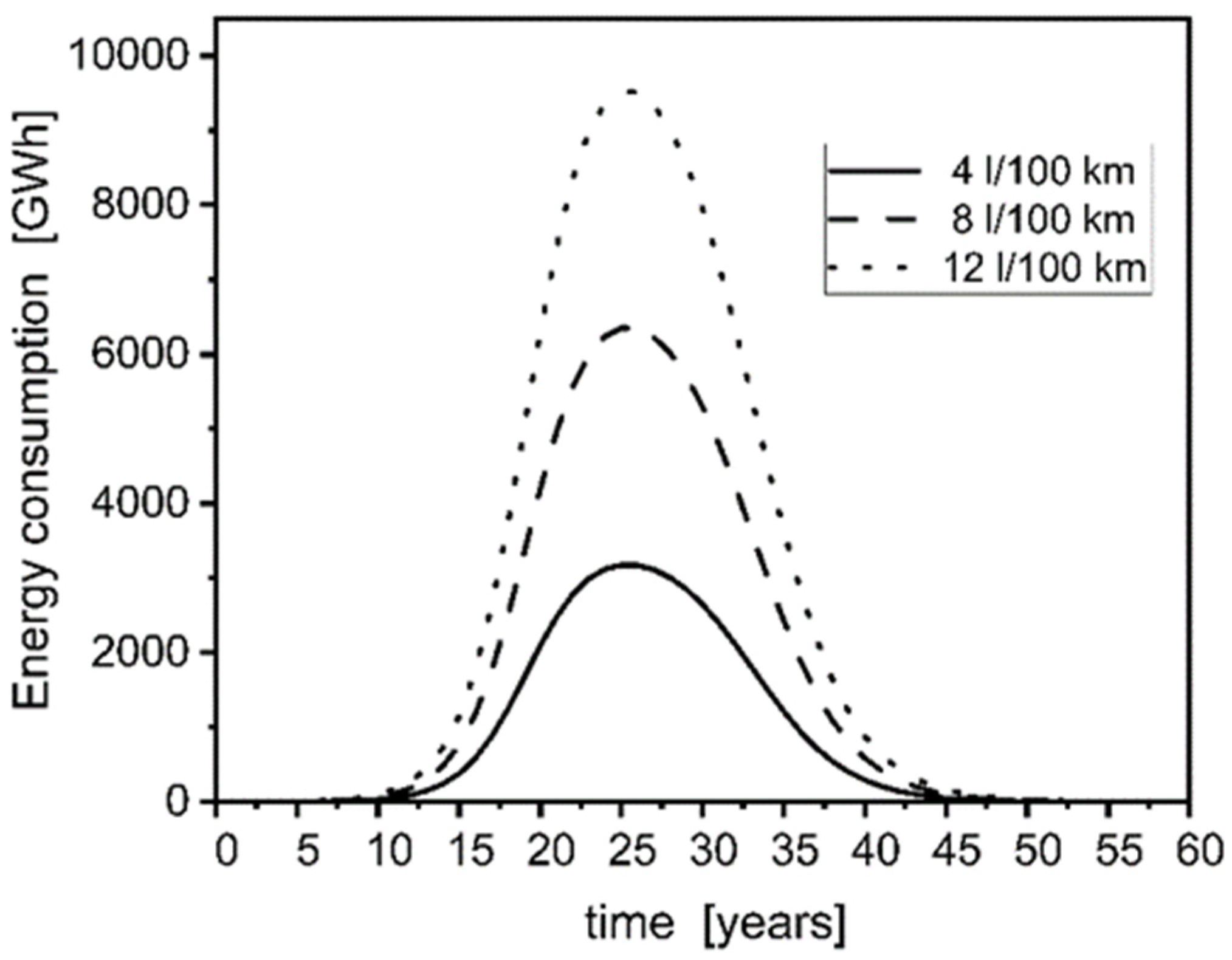
Figure 4 shows energy consumption per year in the case of gasoline fueled vehicles as function of time for classes of cars differing in specific fuel consumption.
The energy demand is obviously proportional to the number of vehicles, distance driven, and specific fuel consumption expressed in liters of fuel needed for 100 km. For the case of cars consuming 12 L per 100 km the energy consumption at maximum reaches almost 10,000 GWh per year when annual mileage is 10,000 km. Obviously, smaller specific consumption gives smaller value of annual energy demand. For the specific fuel consumption equal to 4 L/100 km the maximum energy consumption is slightly above 3000 GWh, what may be assigned to rather small cars or hybrid electric vehicles type HEV, which consume only gasoline and are not charged from external electricity source.
The
Figure 5, and further following figures show total energy consumption i.e., sum of electric and fossil energy demand for existing automobiles according to the three scenarios defined in
Table 1.
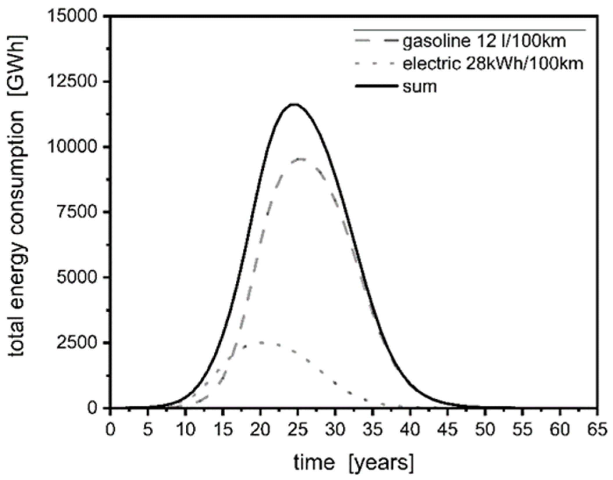
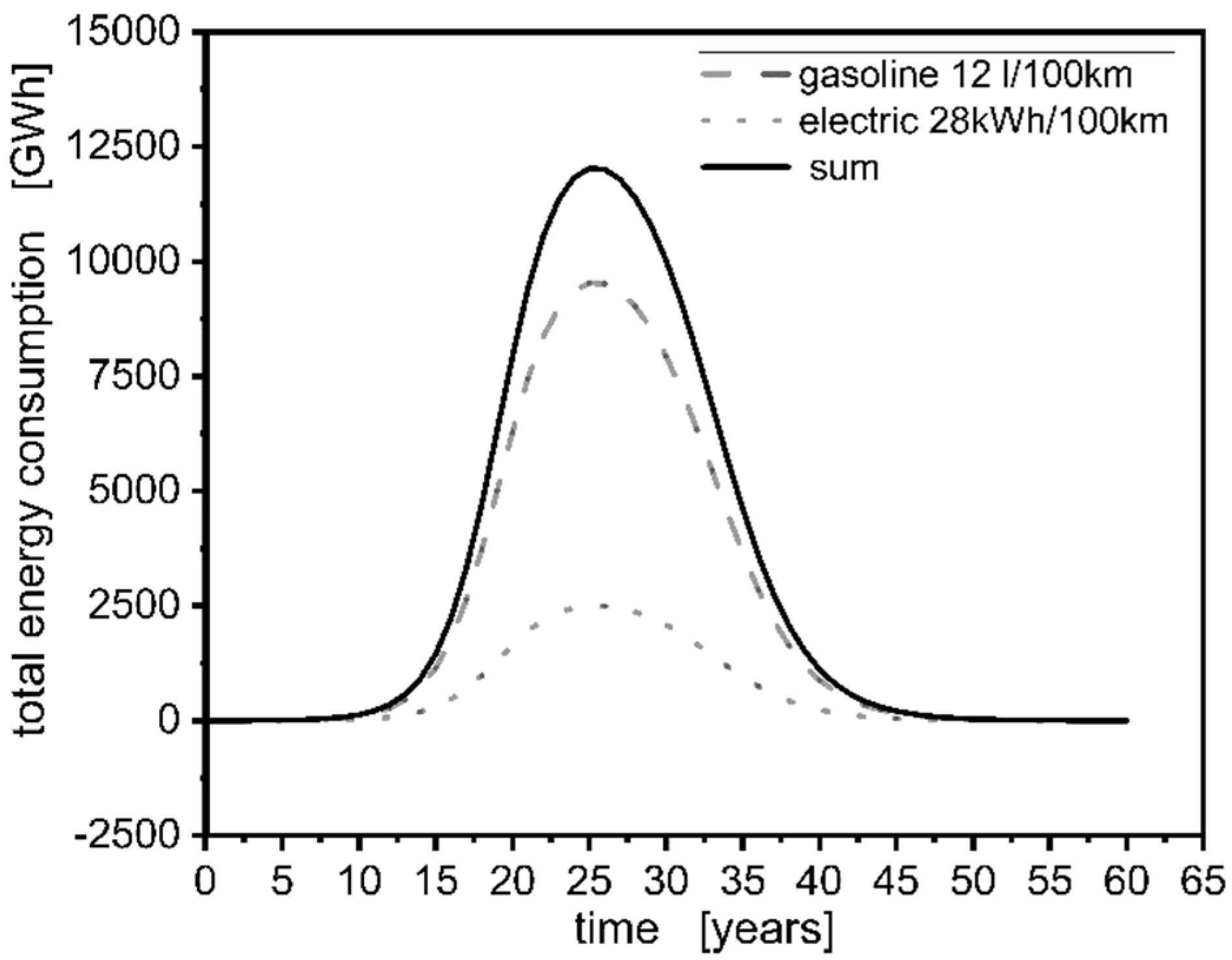
The total energy demand for the first variant of electric vehicles production combined with gasoline fueled ones is shown in
Figure 5. In this case, at the initial period of time the electric cars consume more energy the fossil fuel-powered cars. Maximum of the function for electric cars precedes that for fossil fuel-powered cars. In actual situation it is rather unrealistic because all types of gasoline or diesel-powered cars are already produced for long time, but production of electric cars have started not long time ago. One would rather expect that for the realistic situation the increase of electricity consumption should be accompanied by the decrease of fossil fuel energy consumption, so the curve for electric cars should be shifted to much longer times.
It is also visible that the plot for electric cars for long times disappears earlier than that for gasoline powered cars. One of the reasons is that at the beginning it appears earlier than the curve for gasoline cars. Since the width of both is the same, and the maximum of this curve is shifted to the left, the right end is also shifted to the left. It is evident that energy consumption of electric vehicles in longer times is much smaller than that of gasoline powered ones.
The plot of energy consumption for the second variant is shown in
Figure 6. In this case maxima of both dependencies occur at the same time. The sum of both contributions in this case is generally higher at all times than any of components. The other situation would be expected if both contributing curves would not overlap. Again, it should be mentioned that the sources of both types of energy might be very different or similar (if the electric power stations are using fossil fuels).
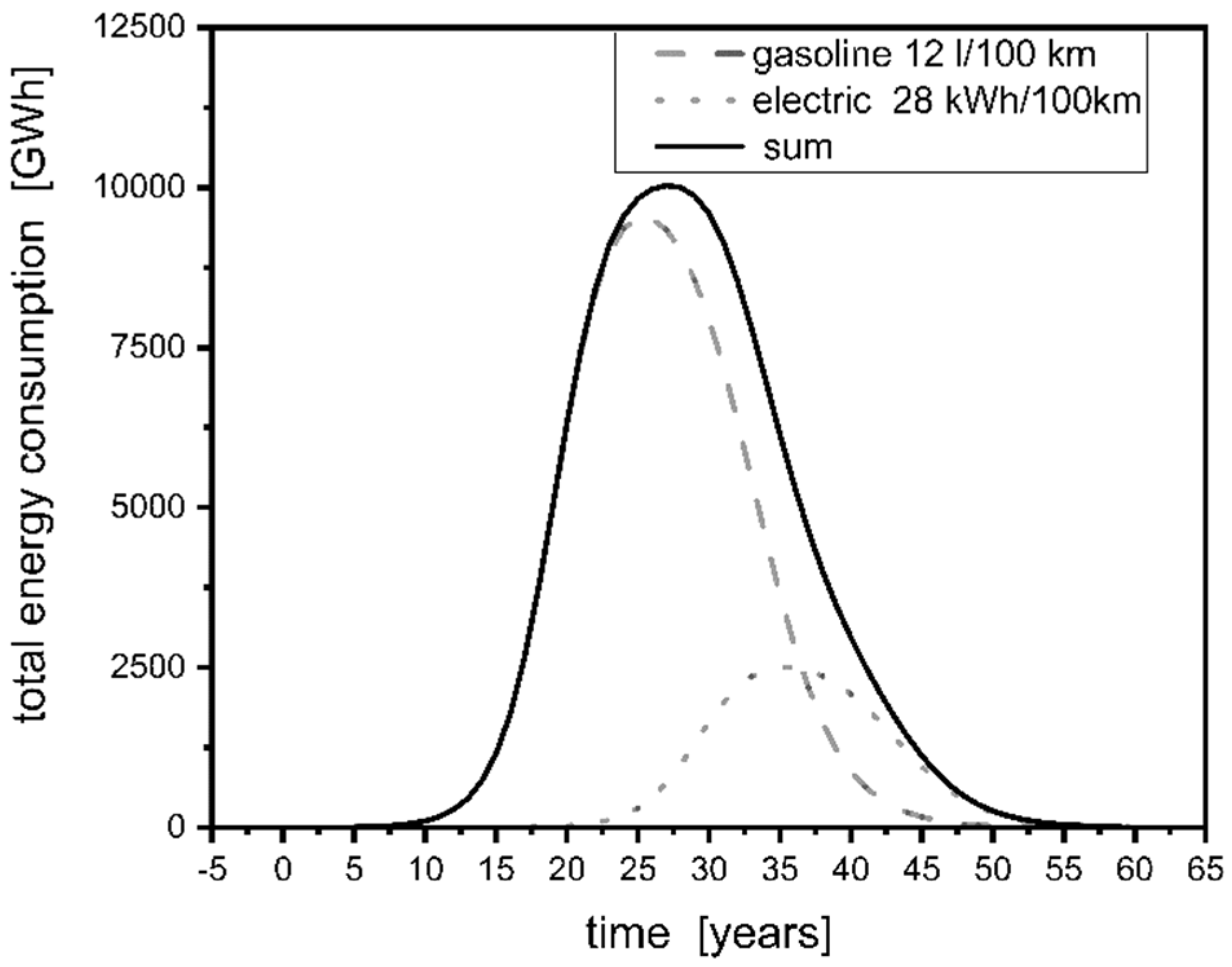
Figure 7, in turn, shows similar functions for the third variant i.e., when the production of electric cars possibly closely corresponds to the decommissioning curve for fossil fuel-powered vehicles. In this case, almost the whole time distribution of existing electric vehicles overlaps with the decreasing part of fossil fuel vehicles. Due to this the left sides of curves for gasoline powered vehicles and the total consumption exactly overlap, while the right (after maximum) side of the total consumption is higher than the consumption computed for gasoline powered vehicles. In this case, also it is worth mentioning that even when the demand for fossil fuel decreases, there exists some additional demand for electricity. This must be covered by additional electricity production.
3.3. Carbon Dioxide Emission
It is well known that energy generation is in most cases linked to carbon dioxide emissions. Although in the case of biomass it is assumed that the emitted carbon dioxide will be re-absorbed by the renewable biomass, but it also temporarily escapes into the atmosphere and, for some time, affects its chemical composition. This is true not only in the cases when a fuel is combusted in the engine of a vehicle, but also occurs when the electric engine of the vehicle is powered by electricity generated in the power station using carbon containing fuel. Usually, electric power stations use various fuels, and there is increasing contribution of alternative sources of energy, such as wind or photovoltaic farms, hydroelectric power plants etc. Consequently, the amount of CO2 emitted to atmosphere substantially varies in European countries.
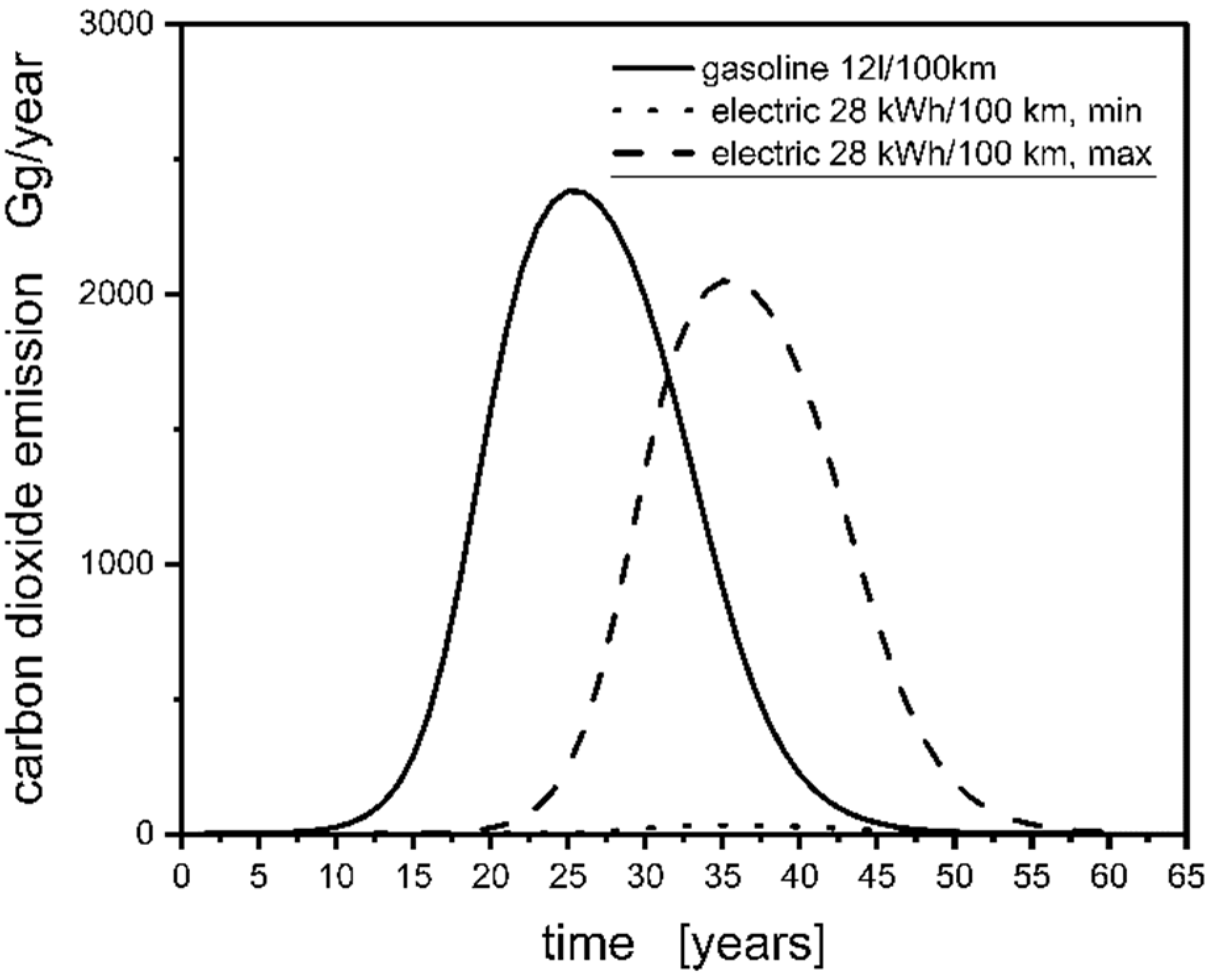
Figure 8 shows contributions of carbon dioxide emissions for gasoline powered cars and electric cars accordingly to the time distributions of vehicle numbers presented at the beginning of the paper. The plots are shown for the cars consuming 12 liters of gasoline per 100 km, for which the maximum value of CO
2 emission reaches about 2400 Gg/year, and vehicles powered by electric engines. For the latter case two values of CO
2 emission were accepted the minimum 0.013 kgCO
2/kWh, and maximal 0.819 kgCO
2/kWh.
The maximum value obtained for the assembly of existing vehicles is about 32 GgCO2/year for the smallest emissions form power stations while about 2050 GgCO2/year for the vehicles using electricity from strongly carbon emitting power plant. The first value is practically negligible as compared to emissions from gasoline powered vehicles, while the value for cars powered from carbon emitting power stations is close to the emissions from gasoline powered cars. This clearly shows that the choice of electric vehicles assures decarbonization of transport only when electricity generation is decarbonized.
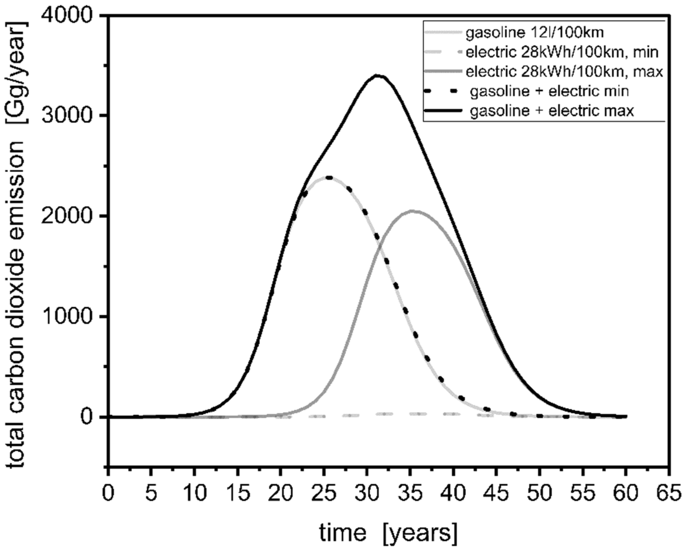
Figure 9 presents total carbon dioxide emissions for above-mentioned variants of coexistence of vehicles and two types of electricity generation.
The figure shows contributions together with the total emissions of carbon dioxide for cars using fossil fuels and those powered by electricity from various power stations. It is clearly seen that the electric cars powered by alternative sources are very slightly contributing to the total emission, but the cars using electricity from fossil fuel-powered electricity generation evidently increase the total emission.
4. Discussion
The logistic function describes the number of products produced from the beginning of production to a given point in time. For products with a finite functioning time, the number of products that have been used up is proportional to the number of products produced. It is, therefore, reasonable to assume that the number of products consumed at a given moment in time is proportional to the number produced at a correspondingly earlier moment in time. This justifies the assumption that the number of products used will also be represented by the logistic function, but shifted to a correspondingly later moment. Consequently, the difference between the number of products produced to date and the number of products used up to that moment determines the number of products that still exists (cf.
Figure 1). The proposed model makes possible to forecast the distribution of existing vehicles for a given instant of time, as well as enabling computation of time dependencies for fuel consumption and carbon dioxide emission.
The results of presented computations show several regularities being observed. First, it is clearly visible that electric vehicles consume less energy than corresponding internal ignition engines. Most probably it is a result of much higher generation of heat from internal ignition engine then electric ones. The heat generated is dissipated in the surroundings, and do not contribute to the work performed by the engine. decrease of population of the old one. However, even in such a case some overlapping occurs. The results presented in this paper can be considered to be ones corresponding to one, specific category of vehicles, or to some average over many categories. For each type of vehicles an increase of their number is observed in the first period followed by the decrease in longer times.
The time distribution function of existing vehicles for those with internal ignition engines, in all performed computations, to some extend overlaps with similar distribution of vehicle with electric engines.
Only in variant 3, shown in
Figure 7, in which the maximum distribution of existing cars is shifted to the right with respect to gasoline cars, the increase in electricity consumption coincides with a decrease in fossil fuels. Even in this case, the energy contribution of fossil fuels is higher than the contribution of electricity consumption. The opposite trend appears late at a time when not only the consumption of fossil fuels, but also electricity decreases as a result of reducing the number of existing vehicles of both types. From practical point of view, it seems reasonable that appearance of the new generation, e.g., electrical vehicles should be correlated with a decrease of population of the old one. However, even in such a case some overlapping occurs. In each case this overlap leads to an increase of total energy consumption. It must be, however, pointed out that each of these generations uses the other type of energy. (The decrease of the electricity consumption is due to the inevitable decrease of population also of electric vehicles after the time when this generation will grow older, and will be replaced with some new generation of vehicles.)
It should be noted that the electricity needed to power one million cars, around 2000 GWh per year, is an additional demand for energy as compared to the normal consumption before the introduction of electric vehicles.
A decrease of energy consumption by automobiles should lead to a decrease of CO2 emissions resulting of transportation. The emission caused by introduction of electric cars although corresponding to a decrease of fossil fuels consumption is very much dependent upon the energy sources used by electric power stations, Values of specific CO2 emission for European countries vary in quite wide range. Since the electricity to power electric cars is additional with respect to normal consumption, it releases also additional emission from electric power stations. Depending on the technology used to generate electricity the power stations contribution may be very small when the alternative sources are used or it may be very high, almost the same as from on the road emissions from cars powered with the fossil fuels. Consequently, the investments in alternative energy sources should accompany implementation of electric vehicles in the large amounts.
The present paper takes into account only the energy consumed by automobiles. This obviously is not the whole problem. The success of one or the other technology is dependent upon the energetic efficiency of the whole system including harvesting of an appropriate resources, converting them into usable form of energy carrier, transportation, and distribution network for that carrier. Each of the parts of that chain may require the input of some amount of energy, or involves some losses of energy. According to [
9] the energetic effectiveness of such system can be estimated based on the formula analogous to EROEI.
where:
ε denotes the total energetic effectiveness of the system,
Eout is the useful energy given off by the system, and
Eini i is values of energy being introduced to the system to assure its operation.
It should be noted that the above indicator is not identical with the thermodynamic efficiency of the converter, because it does not bind the amount of energy supplied for transformation with the amount of energy delivered by the converter.
For the case of a chain of subsystems the partial energetic effectiveness of each subsystem can be written as:
The symbols in the above formula denote: εn—energetic effectiveness of a subsystem; Eout—the energy output from the whole system (the same as in (3)); Einn,j—j-th energy input to the n-th subsystem; Eembn—energy embedded in the infrastructure of the n-th subsystem.
A relation between both quantities can be specified as:
From Equation (7) it can be deducted that the lowest component affects most effectively the value of the total energetic effectiveness.
The classical fuels, including biofuels, as well as electricity production from fossil fuels usually show values of ε > 1, what indicates that the amount of energy obtained from the system is higher than all energy inputs during conversion processes. In the case of hydrogen, most probably it will be a smaller value just because the energy of chemical bonds must be exceeded for the release of free hydrogen from the compounds (water or hydrocarbons). this value will most likely be smaller, ε < 1, because the energy supplied in the form of hydrogen, equal to chemical bonding energy, must be previously delivered to the release of hydrogen from the compounds (water or hydrocarbons). The process will be accompanied by a loss. In addition, for the practical use of hydrogen as a power carrier, additional consumption of significant amounts of energy will be necessary to provide transport to the vehicle filling stations. As a result, the use of hydrogen will be associated with the need to obtain a much larger amount of energy than the one that will be used by vehicles.
Actually, they are three technologies that are supposed to decrease carbon dioxide emissions from transportation:
- (1)
Wider use of biofuels
- (2)
Introduction of electric cars
- (3)
Introduction of hydrogen powered cars equipped with fuel cell.
According to numerous documents published in biofuel literature, they are considered to be neutral vs. carbon dioxide. e.g., [
41,
42]. The argument justifying such opinion is that growing biomass absorbs carbon dioxide from atmosphere, and the same amount releases during combustion. However, it should be taken into account that the process of combustion may be much faster than the process of biomass growth, what causes lack of equilibrium between emission and absorption [
9,
43].
It seems, therefore, that idea of long time use of biofuels has only temporary, transitional meaning. Consequently, the competition between electric and hydrogen powered cars seem to be the trend for the future. The perspectives of both technologies might strongly depend upon the amount of energy needed to provide community with free hydrogen or electricity and to build corresponding infrastructure. The amount of energy needed to build the infrastructure corresponding to the needs of electric or hydrogen powered cars appears to be the important factor determining further development and spreading of these types of vehicles.


