On the Construction of Freeform Volumetric 3D Puzzles

Abstract

We present a simple algorithm for synthesizing volumetric 3D puzzles from a 3D freeform geometric model represented volumetrically as trivariate NURBs functions, $\mathcal{M}$. The construction algorithm is based on the functional composition of puzzle elements, positioned in the domain of $\mathcal{M}$, with $\mathcal{M}$. The puzzle elements can be (heterogeneous) freeform polygonal models or freeform surface or trivariate functions and of arbitrary shape, and can include added joints to neighboring puzzle elements. The proposed approach is demonstrated via several examples of such volumetric puzzles, 3D printed and assembled.

1. Introduction

Three-dimensional volumetric puzzles are popular and intriguing enigmas [1]. Three-dimensional puzzles are classic challenges which can also be found in the arts, for example, the sculpture puzzles by Miguel Berrocal (https://www.puzzlemuseum.com/gallery/berrocal/berrocal.htm, accessed on 14 August 2025). Three-dimensional puzzles improve the visual–spatial reasoning power of the human brain. There are many surprising benefits to assembling puzzles, for all ages and particularly for dementia patients, by improving brain functions in short-term memory (see, for example, [2]). Motivated by these benefits for promoting the computational art, we aim to develop support for classic volumetric puzzles which can employ geometric modeling abilities. A significant portion of industrial 3D artifacts are nowadays geometrically designed with and manufactured from 3D NURBs models [3,4,5]. In this work, we propose a solution which exploits freeform trivariate volumetric representations (V-reps) [6] to construct freeform 3D puzzles which can be fabricated, for example, using additive manufacturing (3D printing).

Much of the geometric industrial designs yield products which are models consisting of (trimmed) NURBs surfaces, where the surfaces’ intersection curves delineate the boundaries of the trimmed surfaces. This common representation, in virtually all contemporary geometric modeling systems, is also known as B-reps, for boundary representations. Yet, B-reps are incapable of representing the interior of the geometry, hence making it highly challenging to construct and control volumetric puzzles which encompass and affect the entire volume of the input model. In this work, we resort to a full volumetric representation (V-rep) to enable this much needed control over the interior of the models.

There are some previous results on the fabrication of 3D puzzles, specifically 3D volumetric puzzles, as we discuss in more detail in Section 2. The main contribution of this work can be summarized as follows:

• A general algorithm is proposed for the synthesis of a 3D volumetric freeform puzzle for a geometric V-rep (and also B-rep surface/polygonal models as will be shown) CAD model, $\mathcal{M}$.
• The puzzle elements can be of any shape as long as the mutually exclusive tiling with these elements resides in, and possibly covers, the domain of $\mathcal{M}$.
• $C^1$-discontinuities in $\mathcal{M}$ are possible and supported.
• The number of puzzle elements is arbitrary, and each element can be of an arbitrary shape, while preserving the continuity with its neighboring elements.
• Texture maps can be applied to the puzzle elements to reconstruct a desired image on the surfaces of $\mathcal{M}$ when realized as a 3D puzzle.

The rest of this work is organized as follows. In Section 2, we briefly review the related previous work. In Section 3, the different steps of the proposed algorithm are explained, and in Section 4, some results are presented, including those of 3D printed and assembled volumetric puzzles. In Section 5, the presented algorithms are extended to also support input models that are polygonal, with the conclusion in Section 6.

2. Previous Work

Considering the long history of geometry and mathematics, it is quite surprising that most geometric puzzles have been designed and crafted only in the last two centuries [1]. Other types of geometric puzzles, such as (planar) jigsaw puzzles, which are simpler and thus have a longer history (over 250 years, presumably invented by John Spilsbury around 1766 (https://en.wikipedia.org/wiki/John_Spilsbury_(cartographer), accessed on 14 August 2025)) than most other types of geometric puzzles. Another recent example are polyomino puzzles [7,8] which are considerably more involved and are even the subject of recreational mathematics [9]. Disentanglement puzzles are yet another variant of known 3D puzzles, typically of only two parts, and in [10] the solutions of such puzzles are explored using 6D configuration spaces.

In computer graphics, the computational design of 3D geometric puzzles has attracted much attention since the introduction of 3D printing technologies, which has made the physical realization of 3D puzzles simpler than ever. A state-of-the-art survey on the currently available range of fabrication capabilities is reported by Bickel et al. [11]. Most of the recent results are in the form of volumetric dissections [7,12], typically planar, and often with interlocking structures [13,14,15,16,17,18] or even with transformable structures [19,20,21], or puzzles that can shape shift between different forms.

Sequin [12] uses several dissection schemes to construct 3D puzzles in a graduate course at UC Berkeley for training the spatial understanding and modeling of solid shapes. While mostly planar dissections are employed in [12], of particular interest are the helicoidal dissections. Mostly planar dissections of 3D meshes are also employed in [13,18]. The work of [13] also designs complex spatial interfaces between puzzle elements aiming at challenging interlockings. In [18], an automatic construction algorithm for burr puzzles is proposed, from the given mesh models.

Song et al. [15] introduce a formal approach to an interlocking mechanism and develop an efficient scheme for constructing decentralized interlocking yet discrete LEGO style brick puzzles. Sun and Zheng [19] introduce dynamically interlocking twisty puzzles which resemble and generalize Rubik’s Cube and its variants to user-supplied 3D models, with, again, mostly planar dissections, to allow the twist motions of the parts. Kita and Saito [14] propose a computational design method for generalizing centrifugal puzzles, by embedding core mechanisms into complex 3D geometric models.

Lo et al. [8] consider the construction of 3D polyomino puzzles over quad-mesh models, as thick shells. The quad-mesh structure on a non-planar surface introduces additional constraints on the possible topological arrangement of polyomino puzzle pieces. Consequently, there is a certain limited class of quad-mesh models which allow the construction of 3D puzzles. Volumetric puzzles are also closely related to volumetric packing, or filling 3-space using 3D elements, which are not necessarily the same. In [22], such a general 3D space filling/packing is presented using the Voronoi tessellation of space.

Considering the dissection-based approaches just discussed, there are virtually no results on the construction of 3D puzzles from freeform spline based geometry. One noted exception is [23], which employs functional composition to synthesize freeform 3D shell jigsaw puzzles. Further, none of the above methods perform the dissections of the input model using freeform general slices.

In this work, we present an approach to the construction of volumetric freeform puzzles from volumetric spline models, while the dissecting geometry can be an arbitrary freeform shape. Assuming the input is a V-rep model $\mathcal{M}$, we construct 3D volumetric puzzles by embedding the elements in the interior of the domain of $\mathcal{M}$ and either functionally composing them with $\mathcal{M}$ [23], or approximating this functional composition using freeform deformations [24] (Henceforth, we refer to both functional composing and its approximating using freeform deformations as composition), yielding the 3D puzzle model and allowing for a continuous level of difficulty in the assembly.

3. Algorithm

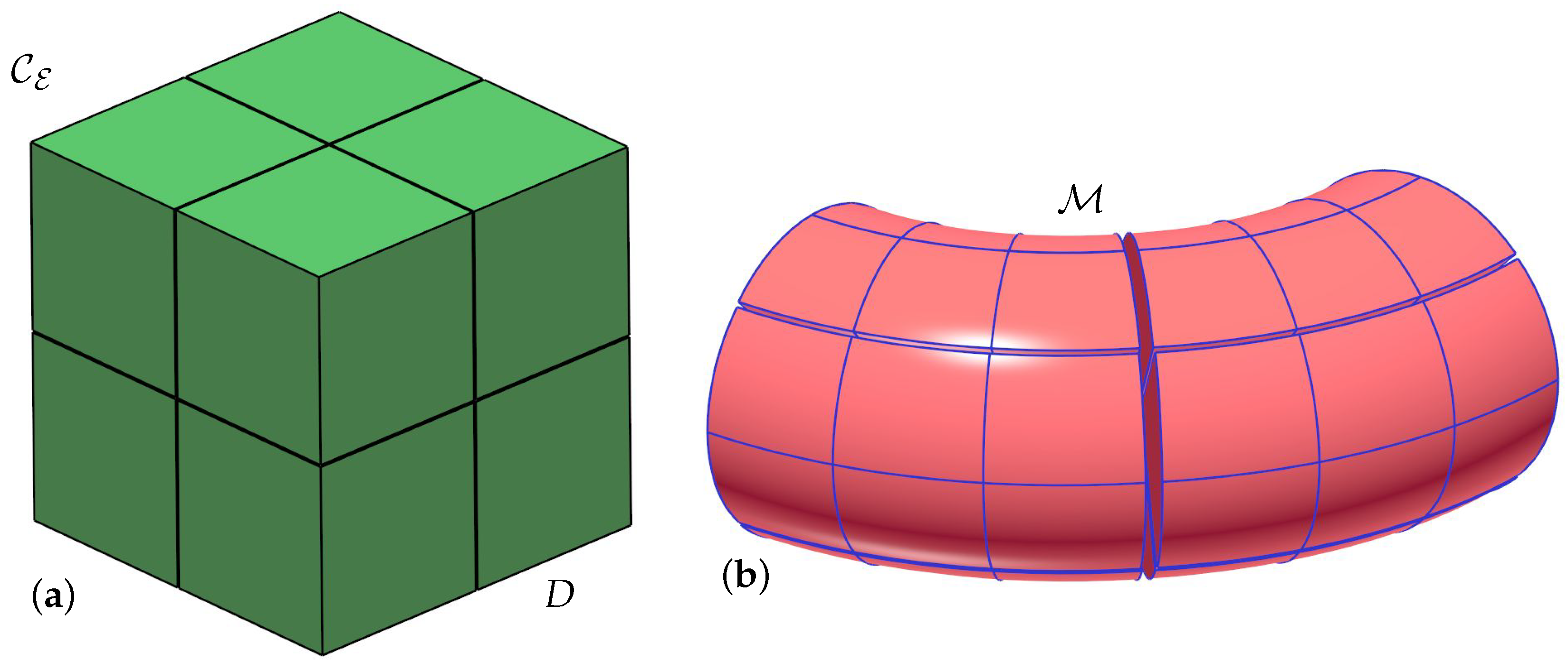
We now present the different steps we perform to create a volumetric puzzle, given a trivariate volumetric model $\mathcal{M}:D\in {IR}^3\to {IR}^3$ (see Figure 1). In our example, this trivariate is divided into two in each of its three parametric directions as can be seen in Figure 2, aiming at eight puzzle pieces. In Section 3.1, we focus on constructing the topology of the puzzle via a division of the domain D of $\mathcal{M}$ to cuboids. Then, in Section 3.2, our simple approach to creating joints between the different puzzle elements is discussed, and in Section 3.3, the randomization of the puzzle elements in the domain D is portrayed, controlling the complexity of the puzzle. Finally, the mapping of the puzzle (and joints) geometry, which is embedded in D, through $\mathcal{M}$ is discussed in Section 3.4.

3.1. Building the Puzzle’s Topology

Any space filling polyhedra, which can be assembled and disassembled together, can be employed here to tile the domain of $\mathcal{M}$, D. For simplicity, herein we fill D with $l\times m\times n$ cuboid elements, $C_E^{l,m,n}$ (see Figure 2), and denote the set of these space filling elements in D as ${\mathcal{C}}_{\mathcal{E}}=\left\{C_{\mathcal{E}}^{l,m,n}\right\},$$\forall l,m,n>0$. Throughout this section, and for clarify of the explanations, we employ a simple demonstration case of a puzzle of eight elements in an arrangement of $l=m=n=2$, while $\mathcal{M}$ is in the shape of a quarter of a torus as in Figure 1 and Figure 2.

3.2. Building the Joints

Adjacent (cuboid) elements from Section 3.1 also require some connectors or joints in between. Again, we choose a simple approach here, to establish the proper connectivity between the puzzle elements. The adjacency graph of the different elements in ${\mathcal{C}}_{\mathcal{E}}$ is monotonically (minimum to maximum) scanned in the three X, Y, and Z directions, independently. For each one of these three directions, we assign pins and holes to every pair of adjacent elements. Further, the locations of the pins/holes in these three directions are carefully defined so no collision (intersection) will occur between two holes, inside a puzzle element. Up to three pins and three holes can exist in one puzzle element. See Figure 3 for an example of two adjacent puzzle elements in the domain D, with pins/holes.

Some V-rep trivariates are periodic, meaning the minimal and maximal boundaries of the domain D in some parametric direction, coalesce in ${IR}^3$. In such cases, pins are also assigned to elements on the maximal boundary, pins which emerge beyond the maximum of D. Similarly, respective holes are assigned in the elements on the minimal boundary of the domain.

As a final remark, these pins and holes will, in the next steps, undergo a mapping through a randomized function, in Section 3.3, and through a mapping to 3-space, in Section 3.4. As long as these mappings are none singular (posses positive Jacobians throughout their domain), the pins and holes will remain compatible and (self-)intersection free.

3.3. Randomizing the Shapes of the Puzzle Elements

Consider the eight puzzle elements in Figure 4a. Employed as is, and up to the different topologies of pins and holes, there will be some elements that are identical. This can simplify the whole complexity of the puzzle’s assembly, as identical puzzle elements could be swapped for yet other valid solution(s).

That said, we could ensure, with high probability, that all elements will be different by constructing a mapping $\mathcal{R}:D\in {IR}^3\to D$, which randomly and continuously deforms the volume inside D (while preserving the boundary of D), and also remaining one-to-one (with a positive Jacobian). Let $\mathcal{R}(u,v,w)$ be a B-spline trivariate function with $q^3$ control points, $R_{ijk},0\le i,j,k<q$, and open end conditions. Randomly perturb the following by some controlled amount:

• All internal control points $R_{ijk},0<i,j,k<q-1$;
• All face-internal control points, in the faces’ planes.

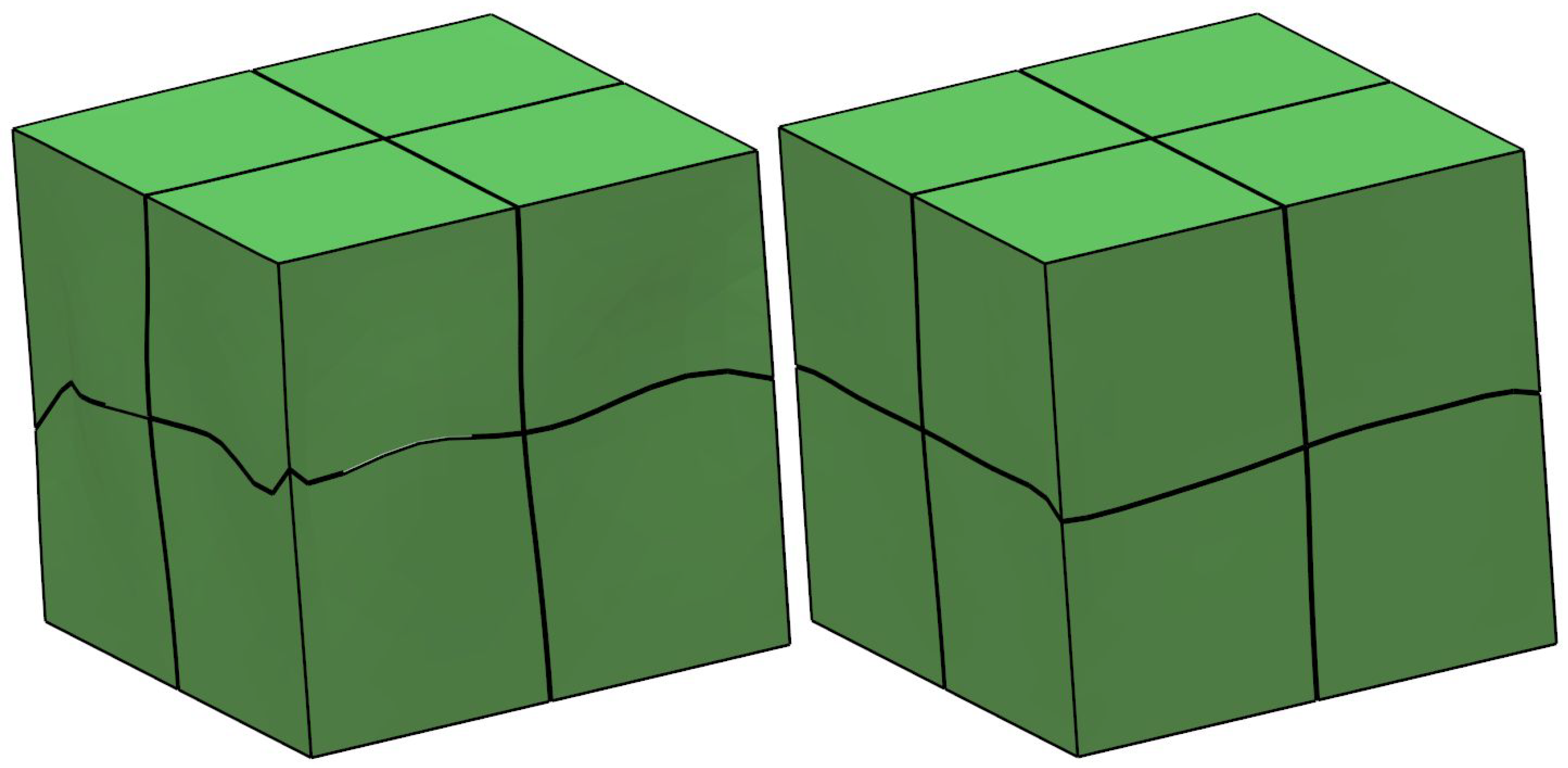
Perturbation 2 requires some clarifications and, for example, for the u minimum face, all control points $R_{0jk},0<j,k<q-1$ will be perturbed in the constant u minimum plane, and the same for the u maximum plane. Then, the same perturbation of face-internal control points will be applied for the v and w minimum/maximum planes. See Figure 4b. Finally, the composition $\overline{{\mathcal{C}}_{\mathcal{E}}}=\mathcal{R}\left({\mathcal{C}}_{\mathcal{E}}\right)$ will create a new set of space filling geometry, inside D, where all elements are no longer cubes/boxes. See Figure 4c. One should note that this perturbation process preserves the six faces, twelve edges, and eight corners of (the boundaries of) D. Finally, this perturbation should be small enough so that we do not violate the bijectivity of the mapping $\mathcal{R}$. While a priori ensuring the bijectivity of $\mathcal{R}$ is challenging, one can robustly verify the positivity of the Jacobian of B-spline trivariate $\mathcal{R}(u,v,w)$, $J_{\mathcal{R}}$, throughout the domain of $\mathcal{R}$, by symbolically computing [25]

$$J_{\mathcal{R}}=\left({\displaystyle \frac{d\mathcal{R}}{du}}\times {\displaystyle \frac{d\mathcal{R}}{dv}}\right)·{\displaystyle \frac{d\mathcal{R}}{dw}},$$

and inspecting all the coefficients of scalar trivariate B-spline $J_{\mathcal{R}}$. If all coefficients are positive, by the convex-hull property of B-spline functions [3], $J_{\mathcal{R}}$ is positive throughout. Such an efficient verification test can provide the end user with immediate feedback when the perturbations are too large.

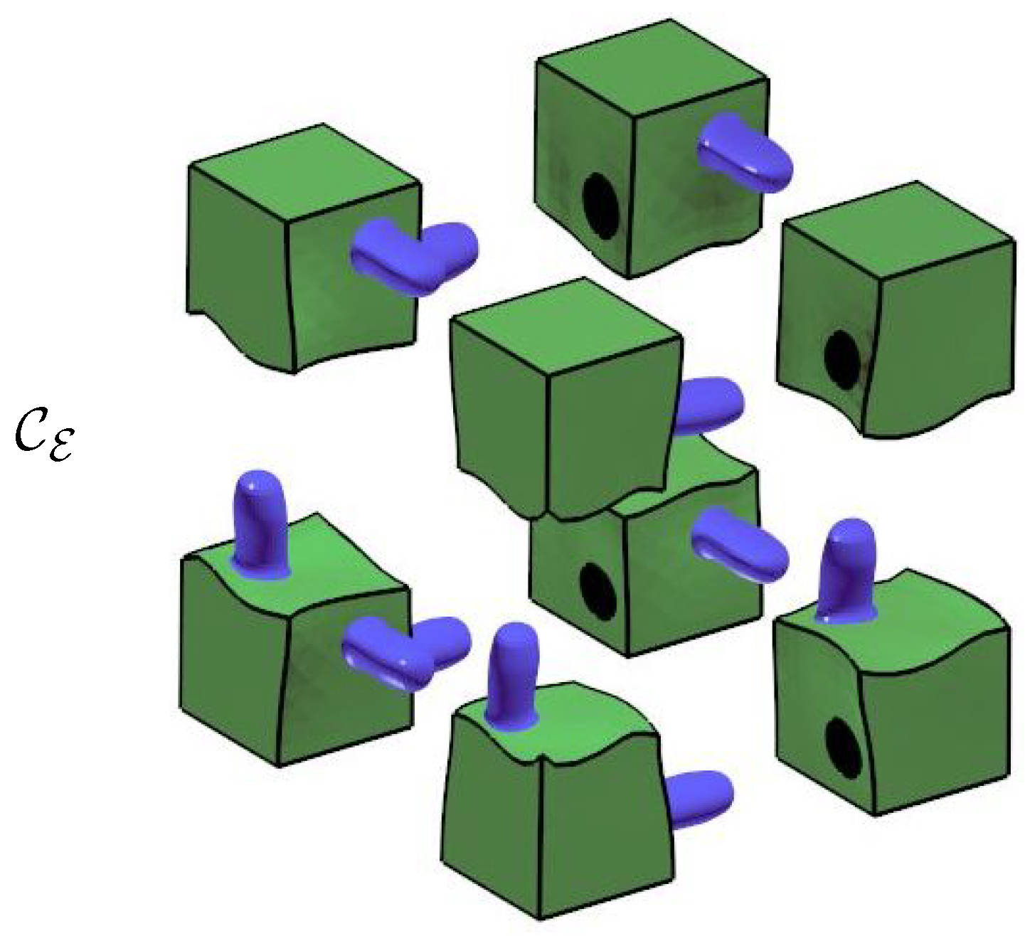
Figure 5 shows again the example from Figure 4c, this time exploded. Worthy of note is the fact that the corresponding pins and holes are undergoing continuous and similar deformations. In other words, the pins in the joints remain compatible with their respective holes, under the deformations of $\mathcal{R}$.

Randomization function $\mathcal{R}$ is a key tool at controlling the level of difficulty of assembling such puzzles. Minute random deformations will leave the puzzle element different yet very much alike. In contrast, large random deformations will leave the puzzle elements highly different. Figure 6 shows two additional examples with various levels of randomness as applied by some $\mathcal{R}$ functions. Compare with Figure 4c.

As a final exemplification of the composition $\overline{{\mathcal{C}}_{\mathcal{E}}}=\mathcal{R}\left({\mathcal{C}}_{\mathcal{E}}\right)$, Figure 7 presents two examples that will be employed shortly, in the following sections. The example in Figure 7a–c is a simple ${\mathcal{C}}_{\mathcal{E}}:=(2\times 2\times 2)$ arrangement of puzzle parts, and will be used in the David model, in the Section 4. The example shown in Figure 7d–f is a more complex ${\mathcal{C}}_{\mathcal{E}}:=(2\times 2\times 8)$ arrangement of puzzle parts that is also periodic in Z, hence the pins at the top in Figure 7d (and corresponding holes at the bottom). This arrangement will be used for the twisted torus model, in the Section 4.

3.4. Mapping to a Freeform 3D Puzzle

The final step, in the puzzle’s construction, maps the randomized arrangement $\overline{{\mathcal{C}}_{\mathcal{E}}}\subset D$ onto the range of $\mathcal{M}$, as $\mathcal{M}\left(\overline{{\mathcal{C}}_{\mathcal{E}}}\right)$. We comment that since $\mathcal{M}$ is rarely an isometry, even if no randomization ($\mathcal{R}$) is applied over ${\mathcal{C}}_{\mathcal{E}}$, in many cases, the puzzle’s elements will all be different.

In the next section, we demonstrate these puzzle creation steps on several model examples, $\mathcal{M}$.

4. Results

We now present some 3D printed results of volumetric puzzles created using the algorithms described in Section 3. The algorithms are implemented using, and are part of, the IRIT (https://gershon.cs.technion.ac.il/irit, accessed on 14 August 2025) modeling kernel, and are written in C. The J55 (https://www.stratasys.com/en/3d-printers/printer-catalog/polyjet/j55-prime, accessed on 14 August 2025) 3D printer from Stratasys is employed in all presented examples. The J55 allows for heterogeneity in both colors and hardness, which we exploit here in 3D printing polymeric materials (https://www.stratasys.com/en/3d-printers/printer-catalog/polyjet/j55-prime/#materials, accessed on 14 August 2025). Each puzzle element is 3D printed in a different random color. Further, the pins (e.g., in blue in Figure 8) are 3D printed flexible in a Shore-A hardness (https://en.wikipedia.org/wiki/Hardness, accessed on 14 August 2025) of around seventy, which is approximately the hardness of a pencil eraser.

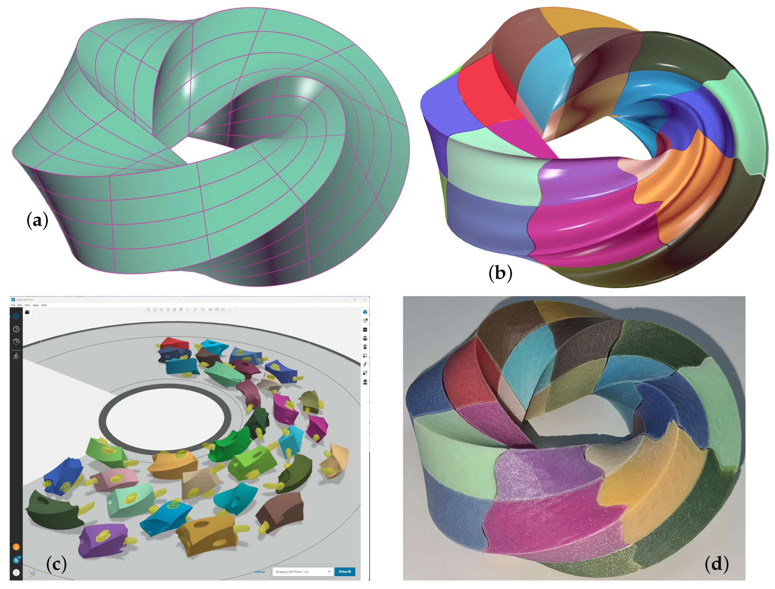
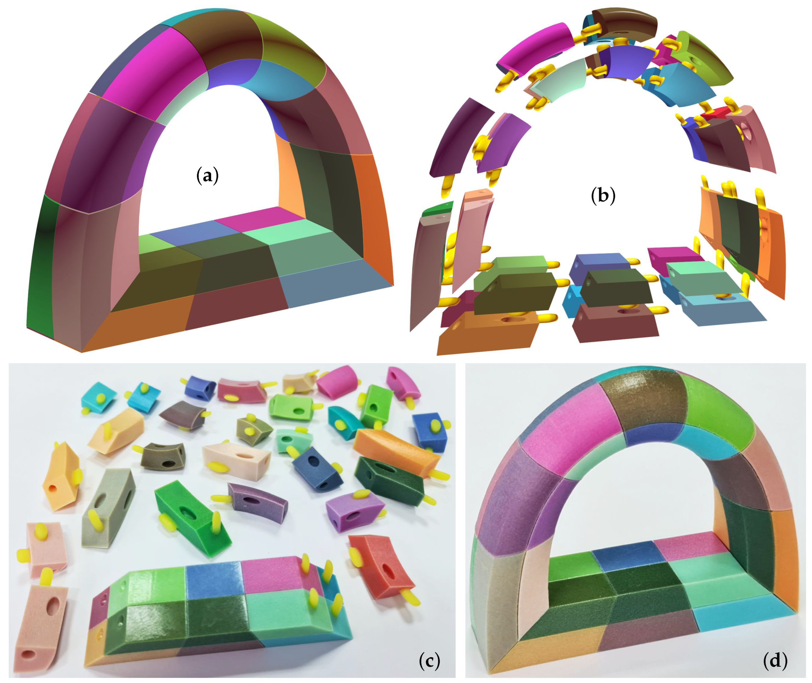
We start with a set of three examples of generalized tori trivariate models with both square (and hence $C^1$ discontinuities) and circular cross sections, shown in Figure 9b, Figure 10a and Figure 11a. The puzzle in Figure 9b is created by dividing domain D into a $2\times 2\times 8$ cuboid arrangement. In all, we have 32 puzzle elements in the puzzle in Figure 9 and some level of randomization is applied, using $\mathcal{R}$. Figure 9b shows the 3D puzzle model, whereas Figure 9c captures the printing layout as is shown in the Stratasys J55 driving software GrabCAD, version 102 (https://grabcad.com). Finally, Figure 9d shows the final 3D-printed and assembled model. Compare Figure 9d with Figure 9b. While all puzzle elements are similar, by exploiting the randomization function $\mathcal{R}$, the adjacent surfaces between neighboring elements in the puzzle are clearly different.

The puzzle in Figure 10a is created by dividing the domain D into a $2\times 2\times 10$ cuboid arrangement. In all, we have 40 puzzle elements and no randomization. (b) shows an exploded view of the puzzle elements, and (c) presents the 3D printed elements of this puzzle, with the linear base already assembled. Then, (d) shows the final 3D printed and assembled model. Compare Figure 10d with Figure 10a.

The puzzle in Figure 11a is also created by dividing domain D into a $2\times 2\times 10$ cuboid arrangement. In all, we have 40 puzzle elements and no randomization: (b) shows an exploded view of the 40 elements of the puzzle, and (c) presents the 3D printed elements of this puzzle, partially assembled. Then, (d) shows the final 3D printed and assembled model. Compare (d) with (a).

These three models, in Figure 9, Figure 10 and Figure 11, have $C^1$ discontinuities, discontinuities which pose little difficulty in the construction of the puzzles. While puzzle elements can have $C^1$ discontinuities in them (as, for example, is the case along the torus in Figure 9), in Figure 10 and Figure 11, the puzzle elements are carefully designed to place the joints at the $C^1$ discontinuities at the two bottom, left and right, sides of these generalized tori.

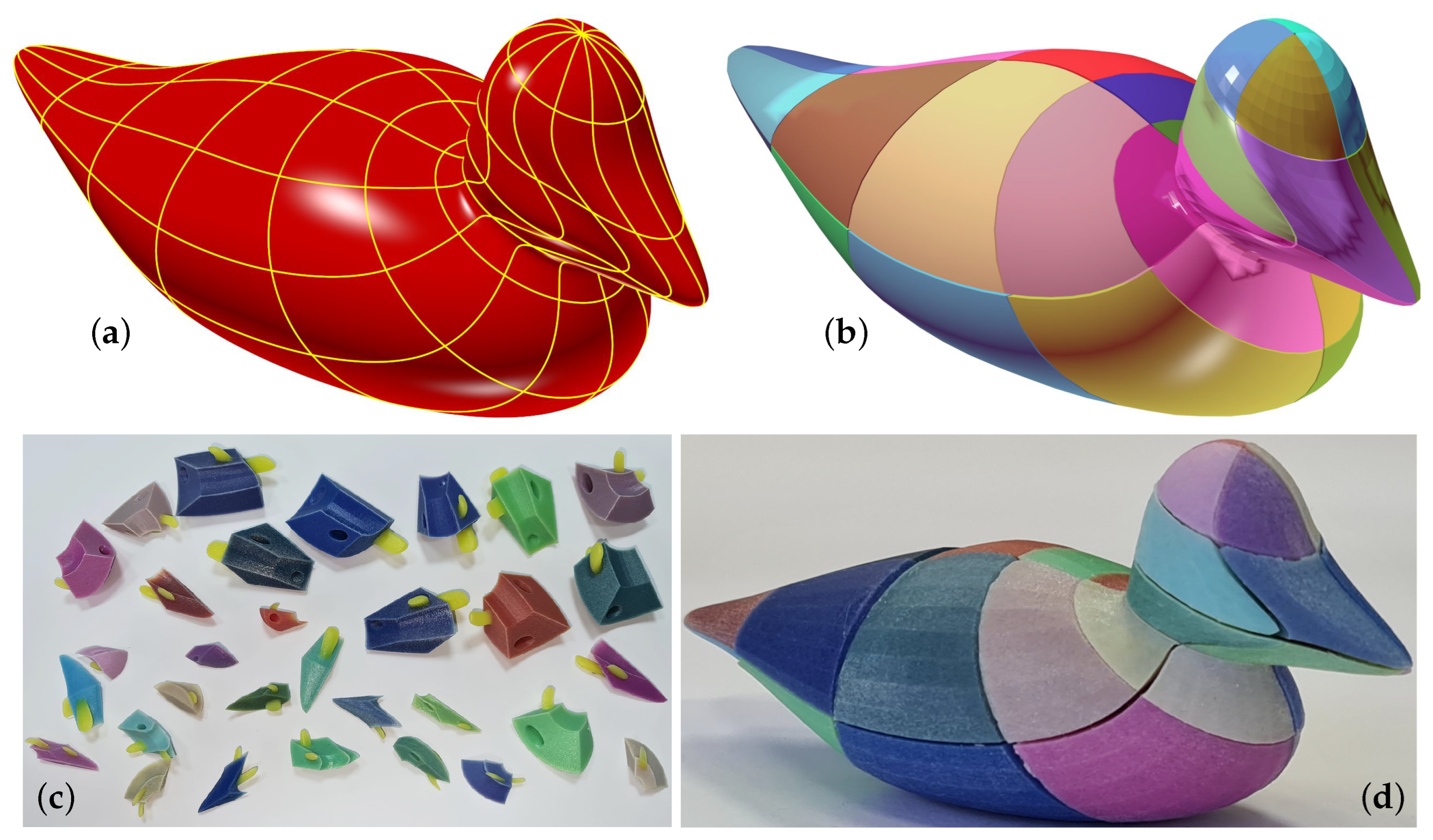
The freeform duck model in Figure 12 is a $4\times 8\times 1$ arrangement of 32 puzzle elements and no randomization $\mathcal{R}$. This puzzle is constructed as a thick shell of the duck, between the shown freeform surface geometry in Figure 12a and the inside surface offset of that geometry.

The earth model in Figure 13 is a $4\times 4\times 1$ arrangement, with 16 puzzle elements and no randomization. Here again, this puzzle is reconstructed as a thick shell, this time of a sphere. Interestingly, herein the earth map is applied over the sphere as a 2D texture map. The correct portions of the earth map are texturing the respective puzzle elements. Figure 13a shows the 3D model of the puzzle. Figure 13b portrays the layout of the 16 puzzle elements in GrabCAD, and finally, Figure 13c presents the 3D printed and assembled puzzle.

5. Extending Algorithms Toward Polygonal Input Models

So far, we assumed that our puzzle is designed using V-rep trivariates. However, the presented approach can also be exploited toward the construction of 3D volumetric puzzles from a B-rep (surface-based or polygonal) input model ${\mathcal{M}}^p$. The puzzle creation process will be augmented, in such a case, with two new pre- and post steps, before and after the stages described in Section 3.1, Section 3.2, Section 3.3 and Section 3.4.

To begin with, a trivariate cage ${\mathcal{M}}^c$ will be created for ${\mathcal{M}}^p$ as a pre-process. See [26] for a survey on the use of cages in computer graphics. Herein, a trivariate function ${\mathcal{M}}^c$ will be constructed which tightly encloses ${\mathcal{M}}^p$ and will serve as a cage for ${\mathcal{M}}^p$. Then, the steps described in Section 3.1, Section 3.2, Section 3.3 and Section 3.4 are applied to ${\mathcal{M}}^c$.

Once the steps from Section 3.1, Section 3.2, Section 3.3 and Section 3.4 are completed, we have a puzzle with the correct topology, embedded in ${\mathcal{M}}^c$. A second, post-process step will be performed, in which the Boolean intersections of the puzzle elements created using ${\mathcal{M}}^c$, with ${\mathcal{M}}^p$ are computed. The end results will capture the geometry of ${\mathcal{M}}^p$ on the outside while preserving the interior topology of the puzzles’ elements from ${\mathcal{M}}^c$ on the inside.

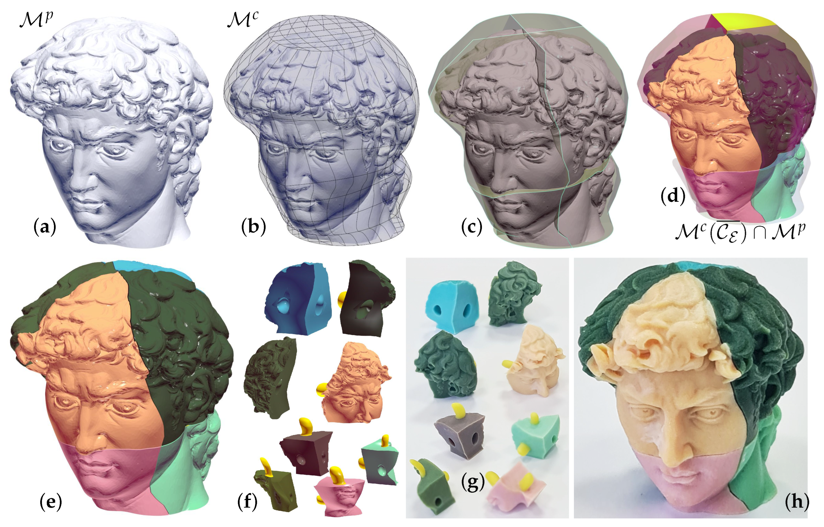
Figure 14 demonstrates this extended process. The model of David’s head, from the Stanford data set (https://graphics.stanford.edu/data/mich, accessed on 14 August 2025), is employed in Figure 14a as our ${\mathcal{M}}^p$ example. A cage ${\mathcal{M}}^c$ is built for this model as a trivariate B-spline function and is shown transparently in (b). (c) presents the division of ${\mathcal{M}}^c$ into $2\times 2\times 2$ puzzle elements, and (d) portrays the Boolean operations steps in converting the puzzle element in ${\mathcal{M}}^c$, ${\mathcal{M}}^c\left(\overline{{\mathcal{C}}_{\mathcal{E}}}\right)$, into the final puzzle elements, by intersecting ${\mathcal{M}}^c\left(\overline{{\mathcal{C}}_{\mathcal{E}}}\right)$ with ${\mathcal{M}}^p$. Some ${\mathcal{M}}^c\left(\overline{{\mathcal{C}}_{\mathcal{E}}}\right)$ puzzle elements in (d) are shown as solid (yellow on the back), some ${\mathcal{M}}^c\left(\overline{{\mathcal{C}}_{\mathcal{E}}}\right)$ puzzle elements are presented as transparent, and the front facial element is shown after this final Boolean intersection.

Figure 14e shows the final computer model of the puzzle, and (f) presents the computer model of the elements of this puzzle, exploded. Then, (g) presents the 3D-printed puzzle elements organized similarly to (f), and finally (h) shows the final 3D-printed and assembled result. Compare (h) with (e).

6. Conclusions and Future Work

This work presented a framework to convert freeform volumetric model $\mathcal{M}$ to a 3D volumetric puzzle, using randomized division of the domain of the trivariates into mutually exclusive cuboid elements which cover the domain D of $\mathcal{M}$. An extended version of this framework was also exploited toward polygonal input objects with a tightly designed trivariate cage.

For simplicity, we chose to initially employ a uniform grid division of the domain D of $\mathcal{M}$. More complex topologies than this uniform grid could and should be considered. We foresee a few possible directions here: First, one can consider other space filling polyhedra such as hexagonal prisms, semi-regular schemes, or even more general space filling geometries such as the approach taken by [22]. Proper joints with the correct topologies should also be designed is such cases.

In addition, a non-regular division of the domain D could be considered as well as is demonstrated in some of the previous work and even in the artwork of Miguel Berrocal. Then, one must also verify the accessibility during the (dis)assembly process—ensuring there is some collision-free dis/assembly sequence to take apart/build the puzzle in 3-space. The general question of an automatic verification of the (dis)assemblability [27] of such puzzles must be further explored, while herein we manually ensure that as part of the puzzle’s design. We note that for puzzles with rigid parts as is the case here, the assembly and disassembly are reversible processes, so the validation of the assemblability also ensures a valid (dis)assembly process. That said, it is quite clear that using the presented algorithm, one can create a 3D puzzle that cannot be (dis)assembled—imagine, for example, a puzzle part that must be (dis)assembled first and yet it will collide with other parts in the process.

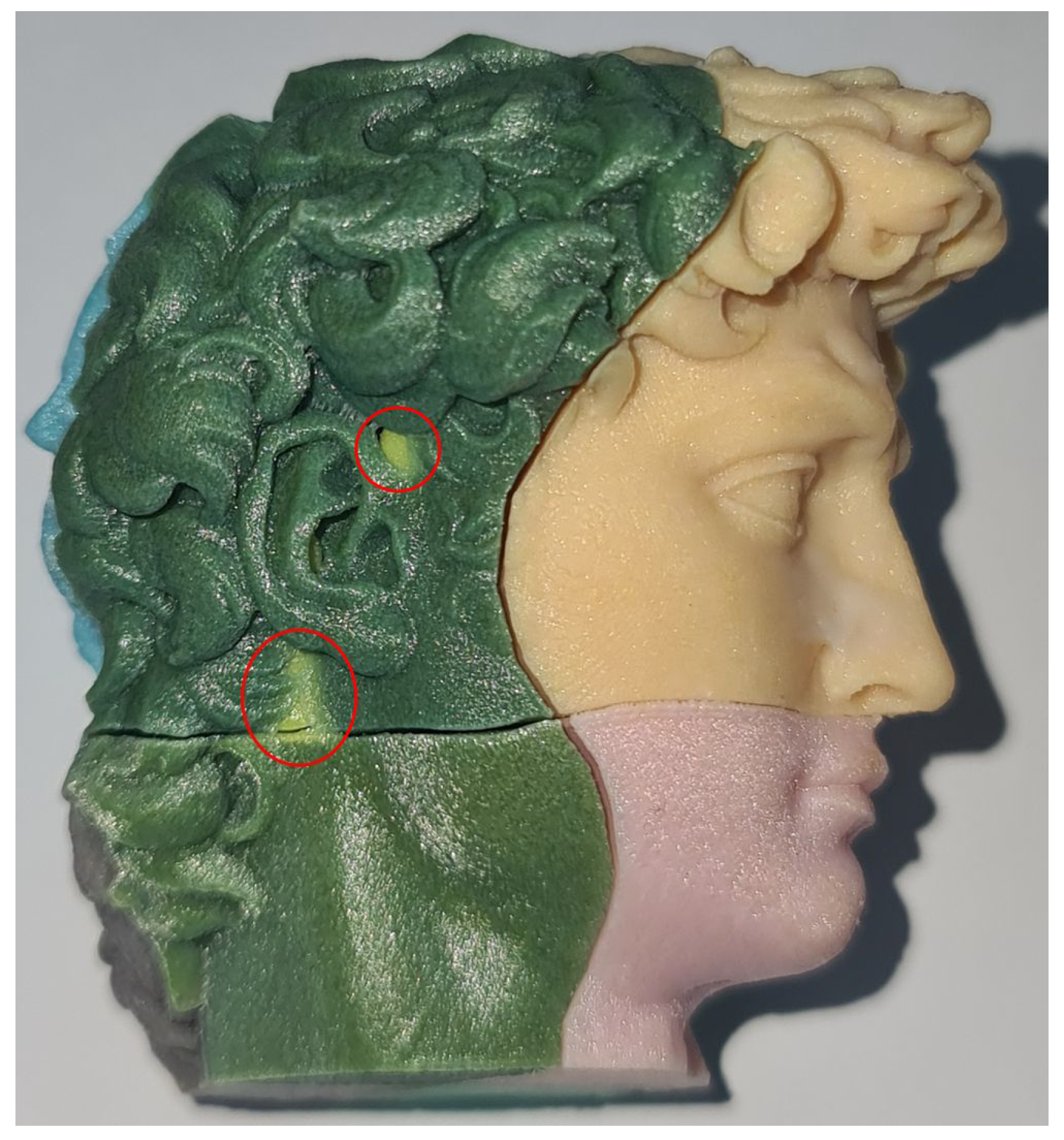
Similarly, we have also assumed a simple approach for joining, exploiting pins and holes. More elaborated connections and joints could be considered as, for example, in [19]. We comment that deep cavities in the model could expose the joints, a clearly undesired effect that should be treated and avoided, possibly by adjusting the locations of the joints on adjacent surfaces. See, for example, Figure 15.

Another direction of improvement concerns the lengths of the pins and holes. As presented, all pins and holes are created with the same dimensions in the domain D of $\mathcal{M}$. Clearly, after the composition, their dimensions can be greatly affected, by the non-distance preserving behaviour of $\mathcal{M}$. A compensation for the dimensions of the pins and holes in the domain D, based on the local magnitudes of the derivatives of $\mathcal{M}$ in its three parametric directions, can greatly alleviate these distortion effects. See, for example, Figure 16.

References

1. Coffin, S. Geometric Puzzle Design; A.K. Peters: Wellesley, MA, USA, 2006. [Google Scholar]
2. Pillai, J.A.; Hall, C.B.; Dickson, D.W.; Buschke, H.; Lipton, R.B.; Verghese, J. Association of crossword puzzle participation with memory decline in persons who develop dementia. J. Int. Neuropsychol. Soc. 2011, 17, 1006–1013. [Google Scholar] [CrossRef] [PubMed]
3. Cohen, E.; Riesenfeld, R.F.; Elber, G. Geometric Modeling with Splines; A.K. Peters: New York, NY, USA, 2001. [Google Scholar]
4. Farin, G. Curves and Surfaces for CAGD: A Practical Guide; Morgan Kaufmann: San Francisco, CA, USA, 2002. [Google Scholar]
5. Hoschek, J.; Lasser, D. Fundamentals of Computer Aided Geometric Design; A.K. Peters: Wellesley, MA, USA, 1993. [Google Scholar]
6. Elber, G. A review of a b-spline based volumetric representation: Design, analysis and fabrication of porous and/or heterogeneous geometries. Comput.-Aided Des. 2023, 163, 103587. [Google Scholar] [CrossRef]
7. Kita, N.; Miyata, K. Computational design of polyomino puzzles. Vis. Comput. 2021, 37, 777–787. [Google Scholar] [CrossRef]
8. Lo, K.; Fu, C.; Li, H. 3D polyomino puzzle. ACM Trans. Graph. 2009, 28, 1–8. [Google Scholar] [CrossRef]
9. Golomb, S. Polyominoes: Puzzles, Patterns, Problems, and Packings, 2nd ed.; Princeton University Press: Princeton, NJ, USA, 1994. [Google Scholar]
10. Zhang, X.; Kry, P.; Vouga, E. On Understanding Disentanglement Puzzles. In Proceedings of the Bridges 2023 Conference, Halifax, NS, Canada, 27–31 July 2023. [Google Scholar]
11. Bickel, B.; Cignoni, P.; Malomo, L.; Pietroni, N. State of the art on stylized fabrication. Comput. Graph. Forum 2018, 37, 325–342. [Google Scholar] [CrossRef]
12. Séquin, C. Prototyping dissection puzzles with layered manufacturing. In Proceedings of the Fabrication and Sculpture Track, Shape Modeling International, College Station, TX, USA, 22–25 May 2012. [Google Scholar]
13. Chen, R.; Wang, Z.; Song, P.; Bickel, B. Computational design of high-level interlocking puzzles. ACM Trans. Graph. 2022, 41, 1–15. [Google Scholar] [CrossRef]
14. Kita, N.; Saito, T. Computational design of generalized centrifugal puzzles. Comput. Graph. 2020, 90, 21–28. [Google Scholar] [CrossRef]
15. Song, P.; Fu, C.; Cohen-Or, D. Recursive interlocking puzzles. ACM Trans. Graph. 2012, 31, 1–10. [Google Scholar] [CrossRef]
16. Song, P.; Fu, Z.; Liu, L.; Fu, C. Printing 3D objects with interlocking parts. Comput. Aided Geom. Des. 2015, 35, 137–148. [Google Scholar] [CrossRef]
17. Tang, K.; Song, P.; Wang, X.; Deng, B.; Fu, C.; Liu, L. Computational design of steady 3D dissection puzzles. Comput. Graph. Forum 2019, 38, 291–303. [Google Scholar] [CrossRef]
18. Yuan, Y.; Zheng, C.; Coros, S. Making burr puzzles from 3D models. ACM Trans. Graph. 2011, 30, 1–8. [Google Scholar] [CrossRef]
19. Sun, T.; Zheng, C. Computational design of twisty joints and puzzles. ACM Trans. Graph. 2015, 34, 1–11. [Google Scholar] [CrossRef]
20. Yuan, Y.; Zheng, C.; Coros, S. Computational design of transformables. Comput. Graph. Forum 2018, 37, 103–113. [Google Scholar] [CrossRef]
21. Zhou, Y.; Sueda, S.; Matusik, W.; Shamir, A. Boxelization: Folding 3D objects into boxes. ACM Trans. Graph. 2014, 37, 1–8. [Google Scholar] [CrossRef]
22. Ebert, M.; Akleman, E.; Krishnamurthy, V.; Kulagin, R.; Estrin, Y. VoroNoodles: Topological Interlocking with Helical Layered 2-Honeycombs. Adv. Eng. Mater. 2024, 26, 2300831. [Google Scholar] [CrossRef]
23. Elber, G.; Kim, M.S. Synthesis of 3D Jigsaw Puzzles over Freeform 2-Manifolds. Comput. Graph. 2021, 102, 339–348. [Google Scholar] [CrossRef]
24. Sederberg, T.W.; Parry, S.R. Free-form deformation of solid geometric models. SIGGRAPH Comput. Graph. 1986, 20, 151–160. [Google Scholar] [CrossRef]
25. Elber, G.; Cohen, E. Second Order Surface Analysis Using Hybrid Symbolic and Numeric Operators. j-tog 1993, 12, 160–178. [Google Scholar] [CrossRef]
26. Ströter, D.; Thiery, J.M.; Hormann, K.; Chen, J.; Chang, Q.; Besler, S.; Mueller-Roemer, J.S.; Boubekeur, T.; Stork, A.; Fellner, D.W. A Survey on Cage-based Deformation of 3D Models. Comput. Graph. Forum 2024, 43, e15060. [Google Scholar] [CrossRef]
27. Shpitalni, M.; Elber, G.; Lenz, E. Automatic Assembly of Three Dimensional Structures via Connectivity Graphs. Ann. CIRP 1988, 38, 25–28. [Google Scholar] [CrossRef]
Figure 1. The input to the puzzle construction algorithm is a volumetric trivariate function M : D I R 3 I R 3 , as is shown in (b) with domain D in (a). Here, M is a quarter of a torus, and the blue curves depict isoparametric curves of M .
Modelling 06 00090 g001
Figure 2. The domain D of M is divided into a set of l × m × n cuboid elements, denoted C E . This set serves as the puzzle elements in D. In (a,b), l = m = n = 2 .
Modelling 06 00090 g002
Figure 3. Two adjacent puzzle elements are shown with their attached pins (in blue) and subtracted holes.
Modelling 06 00090 g003
Figure 4. Given a division of D into puzzle elements as in (a), randomization function R : D I R 3 D I R 3 (b) is employed to deform these puzzle elements, creating (c). See also Figure 2.
Modelling 06 00090 g004
Figure 5. An exploded view of the puzzle elements C E from Figure 4c, after the randomization function R from Figure 4b was applied.
Modelling 06 00090 g005
Figure 6. Two additional application of the randomization function R with varying levels of randomness amounts. Compare with Figure 4c.
Modelling 06 00090 g006
Figure 7. Two examples of exploiting the perturbation function R . (a) shows a puzzle arrangement of C E : = ( 2 × 2 × 2 ) , (b) presents the employed perturbation function R , and (c), the final, deformed arrangement. This example will be used in the David model, in the Section 4. (d) shows a puzzle arrangement of C E : = ( 2 × 2 × 8 ) , (e) shows the employed perturbation function R , and (f), the final, deformed arrangement. This example will be used in the twisted torus model, in the Section 4.
Modelling 06 00090 g007
Figure 8. The geometry C E ¯ in the domain of M , from Figure 4 and Figure 5, is composed with M to yield the final puzzle in 3-space, as M ( C E ¯ ) . (a) shows a minimally exploded result whereas (b) presents a fully exploded view. Compare also with Figure 2b.
Modelling 06 00090 g008
Figure 9. A 3D printed puzzle of a twisted torus V-rep trivariate with a square cross section as is shown in (a). The puzzle consists of 32 elements, all different due to the application of a randomization function R . (b) shows the puzzle’s 3D model, whereas (c) captures the layout of the puzzle elements in the Stratasys GrabCAD software and (d) portrays the final 3D printed and assembled puzzle. Compare (d,b).
Modelling 06 00090 g009
Figure 10. A 3D-printed puzzle of a partially linear generalized V-rep torus with a varying square-to-circle cross section, C 1 discontinuities at the bottom, and with no randomization, is shown in (a). The puzzle consists of 40 elements as can be seen in (b), partially assembled. Some elements are similar geometrically but with different joints. Finally, (c) captures the final 3D printed puzzle, partially assembled (c) and fully assembled (d). Compare (d,a).
Modelling 06 00090 g010
Figure 11. A 3D-printed puzzle of a partially linear generalized V-rep torus with a square-to-circle cross section, C 1 discontinuities at the bottom, and with no randomization, is shown in (a). The puzzle consists of 40 elements as can be seen in the exploded view (b). In (c), the 3D printed and partially assembled puzzle is shown and, finally, (d) captures the final 3D printed and assembled puzzle. Compare (d,a).
Modelling 06 00090 g011
Figure 12. A 3D-printed puzzle of a V-rep Duck (a). Puzzle consists of 32 elements. No randomization is employed in this case, as all puzzle elements are different due to the large variations in the different duck regions. (b) shows the puzzle’s 3D model, whereas (c) captures the layout of the puzzle elements before the assembly, and (d) portrays the final 3D assembled puzzle. Compare (d,b).
Modelling 06 00090 g012
Figure 13. A spherical puzzle with the earth texture. The 3D model is shown in (a) and consists of 16 elements. (b) shows the 3D printing layout of the puzzle’s elements in GrabCAD, and (c) presents the final 3D assembled puzzle. See also the video in https://youtu.be/6wN7nvKKjTQ accessed on 14 August 2025 which shows the assembly process of this puzzle.
Modelling 06 00090 g013
Figure 14. The extended steps in creating a 3D volumetric puzzle of a B-rep polygonal model (a), herein, the head of the David statue from the Stanford dataset. (b) shows a trivariate cage build for (a,c) its division into the elements of the puzzle. Then, (d) partially and (e) fully expose the final computer model off the puzzle elements. (f,g) show the computer models of the 8 individual elements exploded (f) and then 3D printed (g), respectively. Finally, (h) presents the final 3D-printed and assembled puzzle.
Modelling 06 00090 g014
Figure 15. A side view of the puzzle of the David’s head from Figure 14 reveals that deep cavities in the statue expose the yellow joints (see the yellow zones in the red ovals).
Modelling 06 00090 g015
Figure 16. The lengths of the constructed pins depend on the magnitude of the first derivatives of the input V-rep trivariate(s). As a result, some pins end up very short and some are much longer—see the red ovals in the figure. This example is a zoom-in on the bottom row of Figure 11c.
Modelling 06 00090 g016
Disclaimer/Publisher’s Note: The statements, opinions and data contained in all publications are solely those of the individual author(s) and contributor(s) and not of MDPI and/or the editor(s). MDPI and/or the editor(s) disclaim responsibility for any injury to people or property resulting from any ideas, methods, instructions or products referred to in the content.