Stochastic Finite Element Analysis for Static Bending Beams with a Two-Dimensional Random Field of Material Properties

Abstract

This study presents the development and application of the stochastic finite element method (SFEM) to analyze the static response of beams with a two-dimensional (2D) spatially varying elastic modulus. A 2D stationary stochastic field is employed to model the elastic modulus, capturing the material heterogeneity along both the longitudinal and vertical directions of the beam. The weighted integral method is applied to represent the random field as random variables and to compute the element stiffness matrices, while a first-order perturbation technique is utilized to estimate the statistical moments of the nodal displacement vector, including the mean and covariance matrix. This method enhances both computational efficiency and accuracy in capturing material heterogeneity compared to traditional approaches. The precision and effectiveness of the developed SFEM are evaluated through comparisons with Monte Carlo simulations (MCs), demonstrating strong agreement in the analysis of the coefficient of variation (COV) of displacement. A sensitivity analysis is conducted to examine the influence of the correlation length and dispersion of the stochastic field on the COV. The results indicate that the COV generally increases as these parameters grow, with the most significant variations occurring at small correlation lengths. As the correlation length becomes very large, the COV of displacement converges toward the standard deviation of the input stochastic field. Furthermore, the study reveals that the correlation length along the beam’s longitudinal axis has a more pronounced effect on the COV of displacement compared to the vertical correlation length.

1. Introduction

Structural analysis problems are often mathematically represented as systems of differential equations subject to various boundary conditions. The solution of these differential equations can be challenging due to mathematical complexities and limitations. A prevalent numerical method for discretizing the differential equations is the finite element method (FEM). The input factors of the problem encompass model-related factors, such as boundary conditions, loads, and structural property-related factors, including material properties or geometric dimensions of the structure, characterized as parameters with random or uncertain properties [1]. Quantifying the inherent uncertainty in the structure’s response using the standard FEM, which is deterministic, poses a significant challenge. To address this, the stochastic finite element method (SFEM) is employed by integrating the standard FEM with stochastic calculation theory for structural analysis in the presence of uncertain random parameters. SFEM utilizes various strategies to investigate the random response of the structure. Several variations of SFEM have been developed to analyze systems with random factors or uncertain parameters, including the spectral SFEM [2], perturbation approach [3], the weighted integral technique [4], Monte Carlo simulation (MCs) [5], and Neumann series expansion [6,7].

Analyzing structures with random inputs or uncertain parameters typically involves two primary steps. The first step entails representing random factors or parameters as variables or random fields. Various methods have been proposed for representing random fields, such as point discretization [8,9], average discretization [10,11], and series expansion methods [12]. The second primary step is to analyze the stochastic nature of structures using SFEM. While the first step determines the accuracy and suitability of the method, the second step dictates the computational burden and time required for structural analysis [13].

Much research has analyzed beam behavior under various loading conditions, considering deterministic [14,15,16,17] or stochastic material properties [18,19,20,21,22,23,24,25,26,27,28,29]. Deodatis [18] pioneered a technique to determine the upper bound of static response variation in truss and frame structures by calculating the response variance through the variable response and power spectral density function. Deodatis et al. [19] extended this upper bound analysis to plane strain and plane stress problems with 2D random material properties, employing Gaussian quadrature methods for covariance matrix computation. Papadrakakis and Kotsopulos [20] extended stochastic finite element analysis to 2D plane stress problems by combining MCs with the weighted integral method. The local average method was additionally utilized to discretize the random field, facilitating the analysis of three-dimensional solid structures. Chakraborty and Bhattacharyya [21] also expanded the widely used 2D local averaging approach to discretize three-dimensional random fields, representing uncertain structural parameters as homogeneous Gaussian stochastic fields. T.D. Hien [22] developed an SFEM to characterize the behavior of columns with linearly varying cross-sectional areas and spatially random elastic modulus. The weighted integration technique was used to discretize the random field, and the perturbation method was applied to analyze the column’s static response. P.-C. Nguyen et al. [23] analyzed the free vibration problem of beams placed on elastic foundations and beams with longitudinally varying elastic modulus using MCs combined with FEM. While most studies neglect shear deformation, some researchers have employed various shear deformation theories to develop stochastic finite element formulations for analyzing random structural responses. For instance, Gupta and Manohar [24] used a Timoshenko beam theory for the stochastic analysis of curved or straight beams with random material and geometric properties. H.T. Duy et al. [25] extended higher-order beam theories to analyze the random free vibrations of continuous beams on elastic supports with one-dimensional random material properties.

For composite materials, Chen and Guedes Soares [26] conducted a stochastic analysis of multi-layered composite plates with randomly varying material properties using the SSFEM in conjunction with the Karhunen–Loève extension for random field representation. The plate computational theory employed was the first-order shear deformation theory. Sasikumar et al. [27] developed a stochastic analysis framework for composite beams, constructing the probability density function of the non-Gaussian stochastic field based on experimental data to assess beam failure. H.X. Nguyen et al. [28] analyzed the stochastic static response of laminated composite beams and plates using isogeometric analysis combined with the spectral representation method based on MCs. In developing functionally graded material (FGM) beam structures, N. Van Thuan and Chun [29] analyzed the random dynamic response of FGM beams with randomly varying material properties using MCs combined with standard FEM.

Recent research has highlighted the growing interest in analyzing beams with inherent material property randomness. While existing studies typically model the elastic modulus as a one-dimensional random field along the beam’s length, the influence of two-dimensional randomness in material properties has received limited attention. This paper addresses this gap by employing the SFEM to investigate the response variability in static problems involving Euler–Bernoulli beams with 2D uncertain material properties. The proposed SFEM employs weighted integration to discretize the 2D random field of the modulus of elasticity. Subsequently, a first-order perturbation technique is applied to approximate the nodal displacement vector of the beam structure. This approach enables the determination of statistical characteristics of the nodal displacement vector, such as the mean vector and covariance matrix. An independent statistical method based on Monte Carlo simulations (MCs) is developed, building upon the standard FEM and the spectral representation of random fields, to validate the efficacy and accuracy of the SFEM. Furthermore, the study investigates the influence of the correlation distance and the dispersion of the stochastic field on the coefficient of variation (COV) of displacement.

This study introduces an advanced SFEM that combines the weighted integral technique with the first-order perturbation approach, significantly reducing the number of computations compared to traditional statistical methods such as Monte Carlo simulations, thereby shortening computation time and saving computational resources for problems with a large number of elements. In contrast to most previous studies that modeled the elastic modulus as a one-dimensional random field along the beam’s length, the proposed method employs a two-dimensional random field to simulate variations in the elastic modulus in both the longitudinal and transverse directions. This approach enables a more accurate representation of the material heterogeneity, enhancing the reliability of the analysis results. Furthermore, the method’s applicability is not confined solely to the analysis of simply supported bending beams; it can also be extended to more complex structures, including composite structures, intricate connected beams, and other systems with high levels of randomness, thereby meeting the stringent requirements in the design and evaluation of modern engineering structures.

2. Analysis of the Random Static Response of Beams with 2D Uncertainty Elastic Modulus by the SFEM Based on the Weighted Integral Technique

A beam with a span length of L is considered. The beam has a rectangular cross-section with a width of b and a height of h. The beam’s cross-sectional area is represented by A_e. The beam is subjected to a uniformly distributed load q. The origin of the coordinate system is placed at the centroid of the cross-section. The x-axis is aligned with the length of the beam, and the y-axis is aligned with the height of the cross-section. In the classical FEM, the beam structure is discretized into N_e elements, where each element has a length of L_e. The displacement of an element can be approximated using the nodal displacements of the element and shape functions represented by Equation (1).

$$v_i^e=\left[\begin{array}{cccc}{H}_1\left(x_e\right)& H_2\left(x_e\right)& H_3\left(x_e\right)& H_4\left(x_e\right)\end{array}\right]\left\{\begin{array}{c}{p}_1\\ p_2\\ p_3\\ p_4\end{array}\right\}$$

(1)

In Equation (1), the shape function H_i(x_e) represents a basis function, which is defined by Equation (2). The term p_i denotes the i-th component of the element’s displacement vector.

$$\begin{array}{l}{H}_1\left(x_e\right)=1-3{\displaystyle \frac{x_e^2}{{L_e}^2}}+2{\displaystyle \frac{x_e^3}{{L_e}^3}}\\ H_2\left(x_e\right)=x_e-2{\displaystyle \frac{x_e^2}{L_e}}+{\displaystyle \frac{x_e^3}{{L_e}^2}}\\ H_3\left(x_e\right)=3{\displaystyle \frac{x_e^2}{{L_e}^2}}-2{\displaystyle \frac{x_e^3}{{L_e}^3}}\\ H_4\left(x_e\right)=-{\displaystyle \frac{x_e^2}{L_e}}+{\displaystyle \frac{x_e^3}{{L_e}^2}}\end{array}$$

(2)

The beam’s elastic modulus exhibits 2D random variation along the length of the beam and height of the cross-section, as described by Equation (3). In Equation (3), f(x,y) represents a 2D random field. This random field is assumed to be Gaussian, homogeneous, univariate, and has a mean value of zero. Consequently, the element’s elastic modulus in the element’s coordinate system is expressed as shown in Equation (4). E₀ represents the expected value of Young’s modulus.

$$E\left(x,y\right)=E_0\left[1+f\left(x,y\right)\right]$$

(3)

$$E^e\left(x_e,y_e\right)=E_0\left[1+f^e\left(x_e,y_e\right)\right]$$

(4)

Utilizing linear elastic analysis and employing the FEM, the stiffness matrix for the beam element is established, as presented in Equation (5). In this equation, [B] represents the matrix that relates the element’s strain to its displacement.

$${\left[K\right]}^e={\displaystyle {\int }_{V_e}{\left[B\right]}^T{E}^e\left(x_e,y_e\right)\left[B\right]d{V}_e}$$

(5)

Substituting Equation (4) into Equation (5) yields Equation (6), which represents the stiffness matrix of the element with a 2D random elastic modulus. The element’s stiffness matrix is a function of random variables discretized from the random field f(x,y), as described in Equation (7). The matrices appearing in Equation (6) are defined by Equations (8)–(11).

$${\left[K\right]}^e={\left[K\right]}_0^e+{\displaystyle \sum _{i=1}^3\left[\Delta K_i^e\right]Z_i^e}$$

(6)

$$Z_i^e={\displaystyle {\int }_{A_e}{y}_e^2{x}_e^{i-1}{f}^e\left(x_e,y_e\right)d{A}_e}$$

(7)

$${\left[K\right]}_0^e={\displaystyle \frac{E_{0}I}{L_e^3}}\left[\begin{array}{cccc}12& 6L_e& -12& 6L_e\\ & 4L_e^2& -6L_e& 2L_e^3\\ & 12& -6L_e\\ sym& & & 4L_e^2\end{array}\right]$$

(8)

$$\left[\Delta K_1^e\right]={\displaystyle \frac{E_{0}b}{L_e^6}}\left[\begin{array}{cccc}36{L_e}^2& 24{L_e}^3& -36{L_e}^2& 12{L_e}^3\\ & 16{L_e}^4& -24{L_e}^3& 8{L_e}^4\\ & & 36{L_e}^2& -12{L_e}^3\\ sym& & & 4{L_e}^4\end{array}\right]$$

(9)

$$\left[\Delta K_2^e\right]={\displaystyle \frac{E_{0}b}{L_e^6}}\left[\begin{array}{cccc}-144L_e& -84{L_e}^2& 144L_e& -60{L_e}^2\\ & -48{L_e}^3& 84{L_e}^2& -36{L_e}^3\\ & & -144L_e& 60{L_e}^2\\ sym& & & -24{L_e}^3\end{array}\right]$$

(10)

$$\left[\Delta K_3^e\right]={\displaystyle \frac{E_{0}b}{L_e^6}}\left[\begin{array}{cccc}144& 72L_e& -144& 72L_e\\ & 36{L_e}^2& -72L_e& 36{L_e}^2\\ & & 144& -72L_e\\ sym& & & 36{L_e}^2\end{array}\right]$$

(11)

The overall stiffness matrix of the entire beam structure, as represented by Equation (12), is assembled from the element stiffness matrices. It is important to note that the element stiffness matrix is a function of three random variables. Consequently, the overall stiffness matrix of the entire structure is a function of a total of 3 × N_e random variables, as shown in Equation (13), obtained by substituting Equation (6) into Equation (12). Equation (14) defines [K₀], which appears in Equation (13), as the overall structural stiffness matrix evaluated at the expected value of the modulus of elasticity.

$$\left[K\right]={{\displaystyle {\cup }_{e=1}^{N_e}\left[K\right]}}^e$$

(12)

$$\left[K\right]=\left[K_0\right]+{\displaystyle {\cup }_{e=1}^{N_e}{\displaystyle \sum _{i=1}^3\left[\Delta K_i^e\right]Z_i^e}}$$

(13)

$$\left[K_0\right]={{\displaystyle {\cup }_{e=1}^{N_e}\left[K\right]}}_0^e$$

(14)

This study focuses on the static analysis of beam structures within the framework of the SFEM. The governing equation for the static analysis, as represented by Equation (15), involves the overall nodal displacement vector {Δ} of the entire structure and the overall load vector {P}. The overall load vector is considered to be a deterministic quantity in the context of this research.

$$\left[K\right]\left\{\Delta \right\}=\left\{P\right\}$$

(15)

Due to the stochastic nature of the overall stiffness matrix of the entire beam structure, the overall nodal displacement vector of the beam structure is also a function of random variables $\left\{z\right\}={\left\{Z_i^e\right\}}_{i=1,2,3}^{e=1,2,3,\dots ,N_e}$. Employing a Taylor series expansion for the random quantities in Equation (15) around their mean values yields Equations (16) and (17).

$$\left[K\right]\approx \left[K_0\right]+{\displaystyle \underset{e=1}{\overset{N_e}{\cup }}{\displaystyle \sum _{i=1}^3\frac{\mathsf{\partial }\left[K\right]}{\mathsf{\partial }{Z}_i^e}\left(Z_i^e-\overline{Z}\right)}}+{\displaystyle \frac{1}{2}}{\displaystyle \underset{e_1=1}{\overset{N_e}{\cup }}{\displaystyle \underset{e_2=1}{\overset{N_e}{\cup }}{\displaystyle \sum _{i_1=1}^3{\displaystyle \sum _{i_2=1}^3\frac{{\mathsf{\partial }}^2\left[K\right]}{\mathsf{\partial }{Z}_{i_1}^{e_1}\mathsf{\partial }{Z}_{i_2}^{e_2}}}}\left(Z_{i_1}^{e_1}-\overline{Z}\right)\left(Z_{i_2}^{e_2}-\overline{Z}\right)}}+\dots$$

(16)

$$\left\{\Delta \right\}\approx \left\{{\Delta }_0\right\}+{\displaystyle \underset{e=1}{\overset{N_e}{\cup }}{\displaystyle \sum _{i=1}^3\frac{\mathsf{\partial }\left\{\Delta \right\}}{\mathsf{\partial }{Z}_i^e}\left(Z_i^e-\overline{Z}\right)}}+{\displaystyle \frac{1}{2}}{\displaystyle \underset{e_1=1}{\overset{N_e}{\cup }}{\displaystyle \underset{e_2=1}{\overset{N_e}{\cup }}{\displaystyle \sum _{i_1=1}^3{\displaystyle \sum _{i_2=1}^3\frac{{\mathsf{\partial }}^2\left\{\Delta \right\}}{\mathsf{\partial }{Z}_{i_1}^{e_1}\mathsf{\partial }{Z}_{i_2}^{e_2}}\left(Z_{i_1}^{e_1}-\overline{Z}\right)\left(Z_{i_2}^{e_2}-\overline{Z}\right)}}}}+\dots$$

(17)

The first-order and second-order partial derivatives of the overall stiffness matrix appearing in Equation (16) are evaluated at $\left\{z\right\}=0$, similarly to the displacement vector. The mean value of the random variables is denoted by $\overline{Z}$ in Equations (16) and (17). It is noteworthy that $\left\{z\right\}$ is discretized from a zero-mean random field. Consequently, the mean value of the random variables is also zero. Substituting $\overline{Z}=0$ into Equations (16) and (17) yields the following equations:

$$\left[K\right]\approx \left[K_0\right]+{\displaystyle \underset{e=1}{\overset{N_e}{\cup }}{\displaystyle \sum _{i=1}^3\frac{\mathsf{\partial }\left[K\right]}{\mathsf{\partial }{Z}_i^e}{Z}_i^e}}+{\displaystyle \frac{1}{2}}{\displaystyle \underset{e_1=1}{\overset{N_e}{\cup }}{\displaystyle \underset{e_2=1}{\overset{N_e}{\cup }}{\displaystyle \sum _{i_1=1}^3{\displaystyle \sum _{i_2=1}^3\frac{{\mathsf{\partial }}^2\left[K\right]}{\mathsf{\partial }{Z}_{i_1}^{e_1}\mathsf{\partial }{Z}_{i_2}^{e_2}}{Z}_{i_1}^{e_1}{Z}_{i_2}^{e_2}}}}}+\dots$$

(18)

$$\left\{\Delta \right\}\approx \left\{{\Delta }_0\right\}+{\displaystyle \underset{e=1}{\overset{N_e}{\cup }}{\displaystyle \sum _{i=1}^3\frac{\mathsf{\partial }\left\{\Delta \right\}}{\mathsf{\partial }{Z}_i^e}{Z}_i^e}}+{\displaystyle \frac{1}{2}}{\displaystyle \underset{e_1=1}{\overset{N_e}{\cup }}{\displaystyle \underset{e_2=1}{\overset{N_e}{\cup }}{\displaystyle \sum _{i_1=1}^3{\displaystyle \sum _{i_2=1}^3\frac{{\mathsf{\partial }}^2\left\{\Delta \right\}}{\mathsf{\partial }{Z}_{i_1}^{e_1}\mathsf{\partial }{Z}_{i_2}^{e_2}}{Z}_{i_1}^{e_1}{Z}_{i_2}^{e_2}}}}}+\dots$$

(19)

By substituting Equations (18) and (19) into Equation (15) and employing a perturbation technique, we can equate the coefficients on both sides of Equation (15) to obtain the first-order derivative of the nodal displacement vector as represented by the following equation:

$${\displaystyle \frac{\mathsf{\partial }\left\{\Delta \right\}}{\mathsf{\partial }{Z}_i^e}}=-{\left[K_0\right]}^{-1}{\displaystyle \frac{\mathsf{\partial }\left[K\right]}{\mathsf{\partial }{Z}_i^e}}\left\{{\Delta }_0\right\}$$

(20)

The quantity $\left\{{\Delta }_0\right\}$ appearing in Equation (20) represents the overall nodal displacement vector of the entire beam structure corresponding to the deterministic case when the elastic modulus of the beam is equal to the mean value of the random field. Consequently, $\left\{{\Delta }_0\right\}$ is determined as given by Equation (21).

$$\left\{{\Delta }_0\right\}={\left[K_0\right]}^{-1}\left\{P\right\}$$

(21)

Substituting Equations (20) and (21) into Equation (19) yields the first-order approximation of $\left\{\Delta \right\}$, as represented by the following equation:

$$\left\{\Delta \right\}\approx {\left[K_0\right]}^{-1}\left\{P\right\}-{\displaystyle \underset{e=1}{\overset{N_e}{\cup }}{\displaystyle \sum _{i=1}^3{\left[K_0\right]}^{-1}\frac{\mathsf{\partial }\left[K\right]}{\mathsf{\partial }{Z}_i^e}{\left[K_0\right]}^{-1}\left\{P\right\}{Z}_i^e}}$$

(22)

Upon examining Equation (13), it is evident that the overall stiffness matrix of the entire structure is a linear function of the random variables. Consequently, the first-order derivative of the stiffness matrix concerning the random variables evaluated at $\left\{z\right\}=0$ is given by Equation (23), where ${\left[\Delta K_i^e\right]}_E$ is determined from $\left[\Delta K_i^e\right]$ by expanding the sizes of matrix $\left[\Delta K_i^e\right]$ to match the sizes of the overall stiffness matrix of the structure.

$${\displaystyle \frac{\mathsf{\partial }\left[K\right]}{\mathsf{\partial }{Z}_i^e}}={\left[\Delta K_i^e\right]}_E$$

(23)

After substituting Equation (23) into Equation (22), we obtain Equation (24).

$$\left\{\Delta \right\}\approx {\left[K_0\right]}^{-1}\left\{P\right\}-{\displaystyle \underset{e=1}{\overset{N_e}{\cup }}{\displaystyle \sum _{i=1}^3{\left[K_0\right]}^{-1}{\left[\Delta K_i^e\right]}_E{\left[K_0\right]}^{-1}\left\{P\right\}{Z}_i^e}}$$

(24)

The resulting first-order approximations for the mean and covariance matrix of the nodal displacement vector are expressed in Equations (25) and Equation (26), respectively.

$$E\left[\left\{\Delta \right\}\right]=E\left[{\left[K_0\right]}^{-1}\left\{P\right\}-{\displaystyle \underset{e=1}{\overset{N_e}{\cup }}{\displaystyle \sum _{i=1}^3{\left[K_0\right]}^{-1}{\left[\Delta K_i^e\right]}_E{\left[K_0\right]}^{-1}\left\{P\right\}{Z}_i^e}}\right]\simeq {\left[K_0\right]}^{-1}\left\{P\right\}$$

(25)

$$Cov\left[\left\{\Delta \right\},{\left\{\Delta \right\}}^T\right]={\displaystyle \underset{e_1=1}{\overset{N_e}{\cup }}{\displaystyle \underset{e_2=1}{\overset{N_e}{\cup }}{\displaystyle \sum _{i_1=1}^3{\displaystyle \sum _{i_2=1}^3\left\{\begin{array}{l}{\left[K_0\right]}^{-1}{\left[\Delta K_{i_1}^{e_1}\right]}_E{\left[K_0\right]}^{-1}\left\{P\right\}\times \\ {\left\{P\right\}}^T{\left({\left[K_0\right]}^{-1}\right)}^T{\left({\left[\Delta K_{i_2}^{e_2}\right]}_E\right)}^T{\left({\left[K_0\right]}^{-1}\right)}^T\end{array}\right\}E\left[Z_{i_1}^{e_1}{Z}_{i_2}^{e_2}\right]}}}}.$$

(26)

Concerning Equation (7), the expected value of the random variables appearing in Equation (26) is defined as follows:

$$E\left[Z_{i_1}^{e_1}{Z}_{i_2}^{e_2}\right]={\displaystyle {\int }_{A_{e_1}}{\displaystyle {\int }_{A_{e_2}}{x}_{e_1}^{i_1-1}{y}_{e_1}^2{x}_{e_2}^{i_2-1}{y}_{e_2}^{2}E\left[f^{e_1}\left(x_{e_1},y_{e_1}\right),f^{e_2}\left(x_{e_2},y_{e_2}\right)\right]}}d{A}_{e_1}d{A}_{e_2}$$

(27)

The expected value of the random field appearing in Equation (27) is determined through the autocorrelation function of the random field. Consequently, Equation (27) can be rewritten as Equation (28), where $R_{ff}$ is the autocorrelation function of the stochastic field.

$$E\left[Z_{i_1}^{e_1}{Z}_{i_2}^{e_2}\right]={\displaystyle {\int }_{A_{e_1}}{\displaystyle {\int }_{A_{e_2}}{x}_{e_1}^{i_1-1}{y}_{e_1}^2{x}_{e_2}^{i_2-1}{y}_{e_2}^2{R}_{ff}}}d{A}_{e_1}d{A}_{e_2}$$

(28)

Substituting Equation (28) into Equation (26) results in Equation (29), which expresses the covariance matrix of the overall nodal displacement vector for the beam structure. This equation represents the statistical relationships between the displacements of different nodes, considering the uncertainties in the structural parameters.

$$Cov\left[\left\{\Delta \right\},{\left\{\Delta \right\}}^T\right]={\displaystyle \underset{e_1=1}{\overset{N_e}{\cup }}{\displaystyle \underset{e_2=1}{\overset{N_e}{\cup }}{\displaystyle \sum _{i_1=1}^3{\displaystyle \sum _{i_2=1}^3\left\{\begin{array}{l}{\left[K_0\right]}^{-1}{\left[\Delta K_{i_1}^{e_1}\right]}_E{\left[K_0\right]}^{-1}\\ \times \left\{P\right\}{\left\{P\right\}}^T{\left({\left[K_0\right]}^{-1}\right)}^T\\ \times {\left({\left[\Delta K_{i_2}^{e_2}\right]}_E\right)}^T{\left({\left[K_0\right]}^{-1}\right)}^T\end{array}\right\}}}}}{\displaystyle {\int }_{A_{e_1}}{\displaystyle {\int }_{A_{e_2}}{x}_{e_1}^{i_1-1}{y}_{e_1}^2{x}_{e_2}^{i_2-1}{y}_{e_2}^2{R}_{ff}}}d{A}_{e_1}d{A}_{e_2}$$

(29)

The diagonal elements of the nodal displacement vector’s covariance matrix represent the nodal displacements’ variances. Consequently, the variance of nodal displacement can be determined using Equation (30), which extracts the corresponding main diagonal element from the covariance matrix.

$$var\left[\left\{\Delta \right\},{\left\{\Delta \right\}}^T\right]={\displaystyle \underset{e_1=1}{\overset{N_e}{\cup }}{\displaystyle \underset{e_2=1}{\overset{N_e}{\cup }}{\displaystyle \sum _{i_1=1}^3{\displaystyle \sum _{i_2=1}^3\left\{\begin{array}{l}diag\left(\begin{array}{l}{\left[K_0\right]}^{-1}{\left[\Delta K_{i_1}^{e_1}\right]}_E\\ \times {\left[K_0\right]}^{-1}\left\{P\right\}\end{array}\right)\\ \times {\left\{P\right\}}^T{\left({\left[K_0\right]}^{-1}\right)}^T\\ \times {\left({\left[\Delta K_{i_2}^{e_2}\right]}_E\right)}^T{\left({\left[K_0\right]}^{-1}\right)}^T\end{array}\right\}{\displaystyle {\int }_{A_{e_1}}{\displaystyle {\int }_{A_{e_2}}{x}_{e_1}^{i_1-1}{y}_{e_1}^2{x}_{e_2}^{i_2-1}{y}_{e_2}^2{R}_{ff}}}d{A}_{e_1}d{A}_{e_2}}}}}$$

(30)

The COV of mid-span deflections is calculated as the ratio between the standard deviation and the mean of the mid-span deflections.

$$COV={\displaystyle \frac{\sqrt{var{\left[\left\{\Delta \right\},{\left\{\Delta \right\}}^T\right]}_{\frac{L}{2}}}}{\left|E{\left[\left\{\Delta \right\}\right]}_{\frac{L}{2}}\right|}}$$

(31)

The flowchart illustrating the stochastic static analysis of beams with a two-dimensional randomly varying elastic modulus is presented in Figure 1. The first-order perturbation technique truncates the Taylor series at the linear term, limiting its ability to capture higher-order nonlinear effects. This simplification can lead to an underestimation of response variability and may inadequately model non-Gaussian input distributions, particularly in systems with significant uncertainty or strong nonlinearity.

3. Analysis of the Random Static Response of Beams with 2D Uncertainty Elastic Modulus Monte Carlo Analysis

Monte Carlo simulation is a widely employed technique for directly approximating the solution of stochastic partial differential equations governing random beam problems. This study leverages the spectral representation method [30] to characterize 2D random variability of Young’s modulus throughout the beam’s height and length. Two-dimensional Gaussian, uniform, and univariate random fields with zero mean are represented as a finite sum of harmonic functions with definite amplitudes and random phases, as depicted in Equation (32)

$$f\left(x,y\right)=\sqrt{2}{\displaystyle \sum _{n_1=0}^{N_1-1}{\displaystyle \sum _{n_2=0}^{N_2-1}\left[A_{n_1{n}_2}\cos \left({\mathrm{\Omega }}_{1,n1}x+{\mathrm{\Omega }}_{2,n2}y+{\mathrm{\Phi }}_{n_1{n}_2}^{\left(1\right)}\right)+B_{n_1{n}_2}\cos \left({\mathrm{\Omega }}_{1,n1}x-{\mathrm{\Omega }}_{2,n2}y+{\mathrm{\Phi }}_{n_1{n}_2}^{\left(2\right)}\right)\right]}}$$

(32)

The formulas below define the parameters in Equation (32):

$$\begin{array}{l}{A}_{n_1{n}_2}=\sqrt{2S_{ff}\left({\mathrm{\Omega }}_{1,n_1},{\mathrm{\Omega }}_{2,n_2}\right)\Delta {\mathrm{\Omega }}_1\Delta {\mathrm{\Omega }}_2}\\ B_{n_1{n}_2}=\sqrt{2S_{ff}\left({\mathrm{\Omega }}_{1,n_1},-{\mathrm{\Omega }}_{2,n_2}\right)\Delta {\mathrm{\Omega }}_1\Delta {\mathrm{\Omega }}_2}\end{array}$$

(33)

$$\begin{array}{l}{\mathrm{\Omega }}_{1,n_1}=n_1\Delta {\mathrm{\Omega }}_1;\hspace{0.33em}\hspace{0.33em}\hspace{0.33em}{\mathrm{\Omega }}_{2,n_2}=n_2\Delta {\mathrm{\Omega }}_2\\ \Delta {\mathrm{\Omega }}_1={\displaystyle \frac{{\mathrm{\Omega }}_{1u}}{N_1}};\hspace{0.33em}\hspace{0.33em}\Delta {\mathrm{\Omega }}_2={\displaystyle \frac{{\mathrm{\Omega }}_{2u}}{N_2}}\\ n_1=0,1,2,\dots ,N_1-1;n_2=0,1,2,\dots ,N_2-1\end{array}$$

(34)

In Equation (32), ${\mathrm{\Phi }}_{n_1{n}_2}^{\left(1\right)}$ and ${\mathrm{\Phi }}_{n_1{n}_2}^{\left(2\right)}$ are initial random phases, modeled as uniformly distributed random variables in the interval $\left[0,2\pi \right]$. In Equation (33), $S_{ff}$ represents the power spectral density function of the 2D stochastic Young’s modulus field, as defined in Equation (35).

$$S_{ff}\left({\mathrm{\Omega }}_1,{\mathrm{\Omega }}_2\right)={\sigma }_f^2{\displaystyle \frac{d_x{d}_y}{4\pi }}\exp \left[-{\left({\displaystyle \frac{d_x{\mathrm{\Omega }}_1}{2}}\right)}^2-{\left({\displaystyle \frac{d_y{\mathrm{\Omega }}_2}{2}}\right)}^2\right]$$

(35)

In Equation (35), σ_f represents the standard deviation of the 2D random field. d_x and d_y represent the correlation lengths along the x-axis and y-axis, respectively. ${\mathrm{\Omega }}_{1u}$ and ${\mathrm{\Omega }}_{2u}$ represents the upper cut-off limit of wave numbers. When the angular frequency exceeds the upper limit cut-off frequency, the power spectral density function becomes zero. In cases of mathematical difficulties, the upper limit of the cut-off frequency is determined as follows:

$${\displaystyle {\int }_0^{{\mathrm{\Omega }}_{1u}}{\displaystyle {\int }_{-{\mathrm{\Omega }}_{2u}}^{{\mathrm{\Omega }}_{2u}}{S}_{ff}\left({\mathrm{\Omega }}_1,{\mathrm{\Omega }}_2\right)d{\mathrm{\Omega }}_{1}d{\mathrm{\Omega }}_2}}=\left(1-\zeta \right){\displaystyle {\int }_0^{\infty }{\displaystyle {\int }_{-\infty }^{\infty }{S}_{ff}\left({\mathrm{\Omega }}_1,{\mathrm{\Omega }}_2\right)d{\mathrm{\Omega }}_{1}d{\mathrm{\Omega }}_2}}$$

(36)

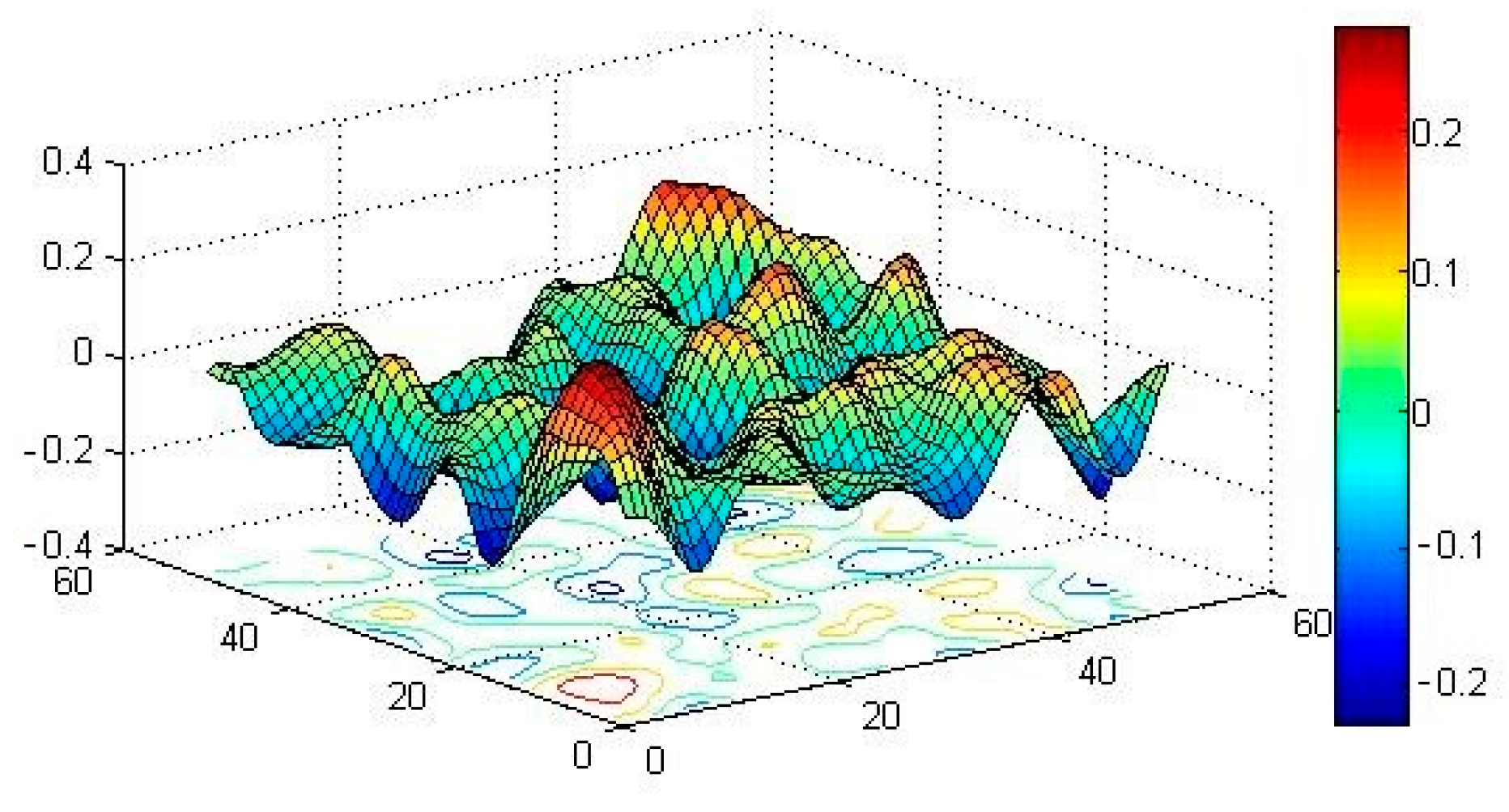
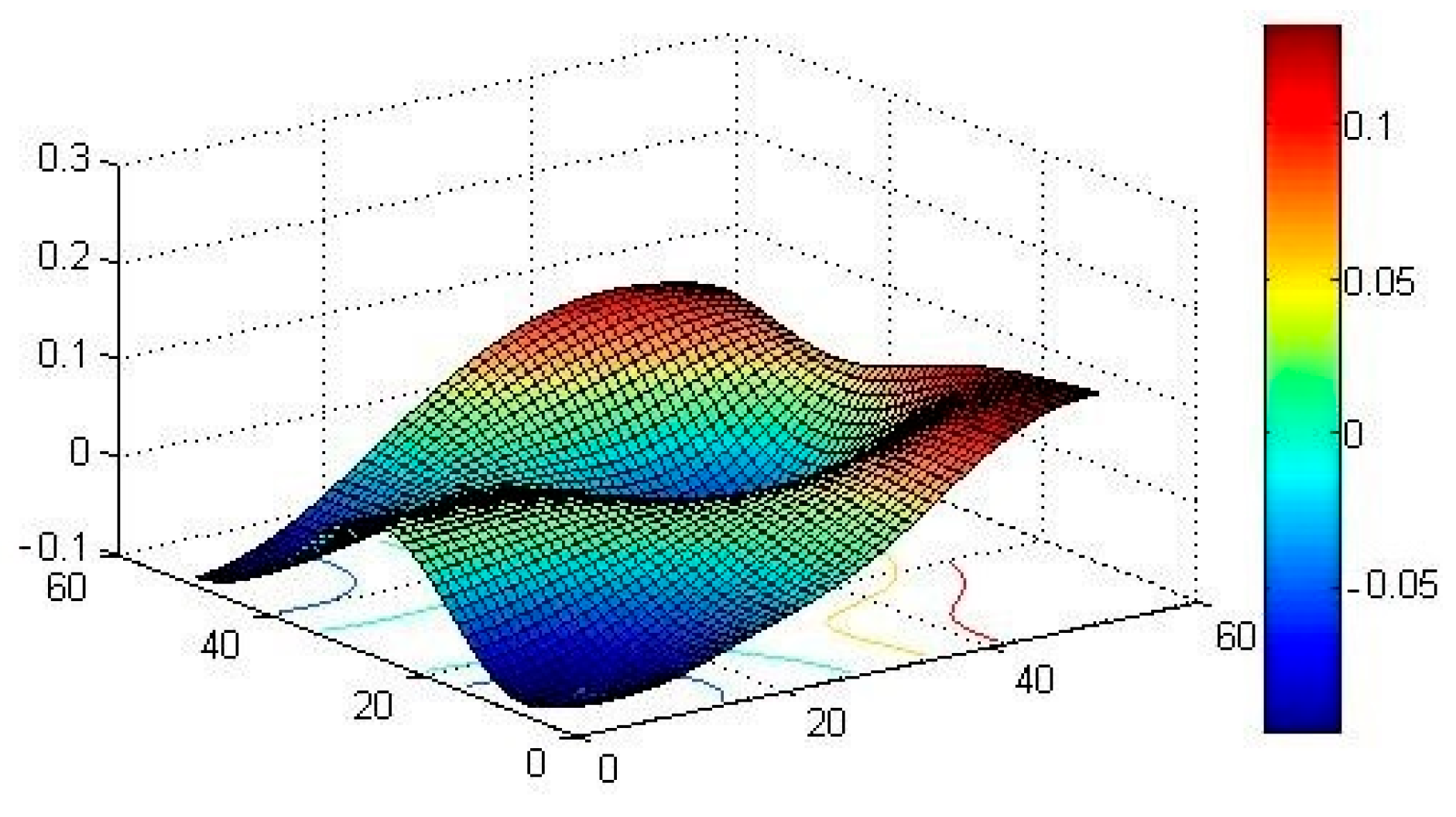
where $\zeta \ll 1$ represents an acceptable relative error in analytical calculations. In this study, we employed Equation (32) to generate realizations of a Gaussian, homogeneous, and univariate stochastic field with zero mean. The autocorrelation function of the 2D Gaussian stochastic field is given by Equation (37).

$$R_{ff}\left(x_2-x_1,y_2-y_1\right)={\sigma }_f^2\exp \left[-{\left({\displaystyle \frac{x_2-x_1}{d_x}}\right)}^2-{\left({\displaystyle \frac{y_2-y_1}{d_y}}\right)}^2\right]$$

(37)

Figure 2, Figure 3 and Figure 4 depict sample realizations of the elastic modulus random field corresponding to different correlation length scenarios, which were obtained using the spectral representation method as described in Equation (32).

To verify and compare the static response analysis of beams using the SFEM, the MCs method [31] is employed in this study. The element stiffness matrices are determined to correspond to the realizations of a 2D stochastic field using the Gaussian integral technique. The main steps involved in the MC simulation procedure are as follows: (1) define the random input quantity as the 2D random elastic modulus; (2) identify the statistical parameters and generate an ensemble of random elastic modulus field realizations; (3) apply classical FEM to analyze the static response of the structure, obtaining an ensemble of structural response data; and (4) utilize standard statistical analysis tools on the obtained data set to derive the statistical characteristics of the structural static response.

MC simulation is a widely used method for uncertainty quantification due to its simplicity and general applicability to complex stochastic problems. Its primary advantage lies in its non-intrusive nature, allowing direct application to existing deterministic solvers without modifications. However, MCs suffers from a slow convergence rate of O(1/$\sqrt{N}$), necessitating a large number of samples—often in the range of 10³ to 10⁶—to obtain statistically reliable results. This high computational cost becomes particularly problematic for problems with fine spatial discretization, as each sample requires solving a full deterministic finite element problem. Moreover, MCs demands finer meshes when the correlation length of the stochastic field decreases, increasing the overall computational burden. Despite these challenges, MCs remains a robust approach for highly nonlinear problems and rare-event analysis, where intrusive methods such as the SFEM may struggle with capturing extreme-value statistics or discontinuities in response distributions. Various variance reduction techniques, such as importance sampling, Latin hypercube sampling, or quasi-Monte Carlo methods, have been developed to improve efficiency [32]. Additionally, adaptive mesh refinement strategies can further optimize computational performance by balancing accuracy and computational cost across different spatial resolutions.

4. Results and Discussion

The following example is considered: a simple beam with a rectangular cross-section subjected to a uniformly distributed load q = 10 kN/m. The beam’s geometric dimensions are L = 5 m, h = 0.4 m, and b = 0.25 m. The mean value of the elastic modulus is E₀ = 32 × 10³ MPa. The elastic modulus can be represented as a 2D Gaussian random field that is homogeneous, univariate, and has a zero mean. Figure 5 illustrates a beam with a 2D random elastic modulus, where the elastic modulus is represented using the spectral method.

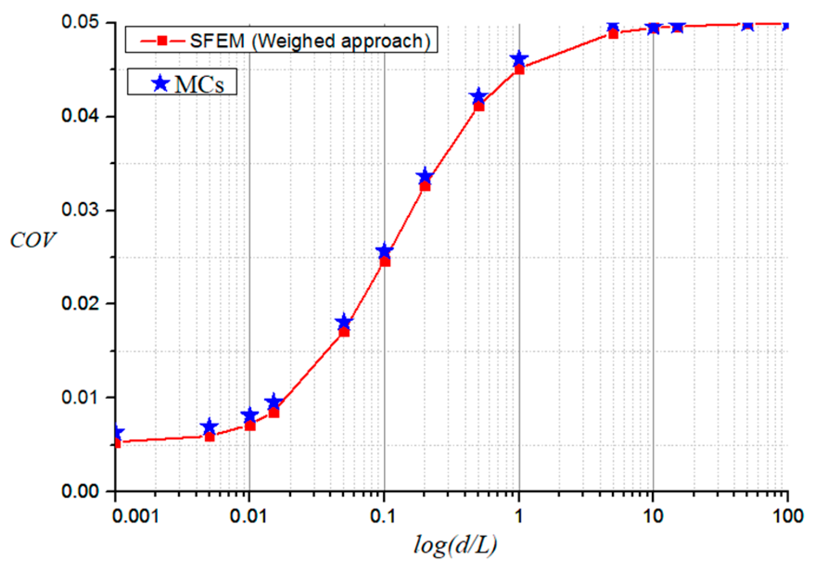
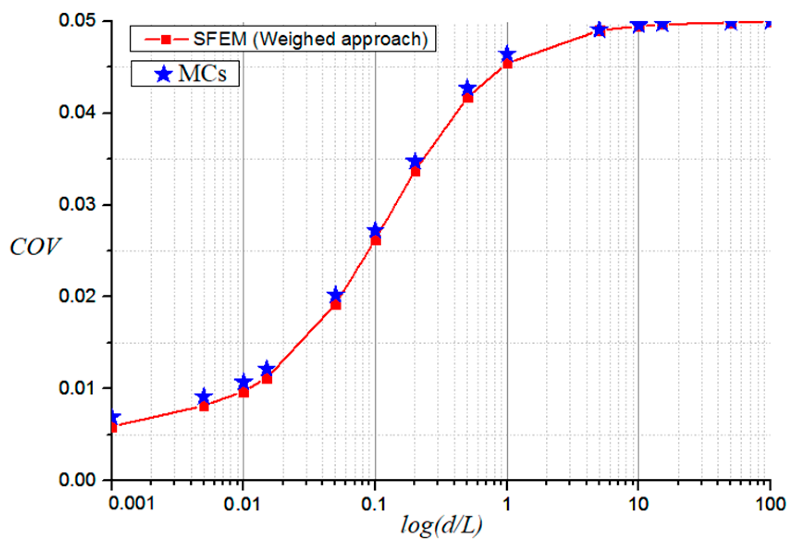
In this section, we investigate the performance of the newly developed SFEM based on weighted integration by comparing it to the established MCs. We evaluate the coefficient of variation (COV) of displacement for three scenarios: d_x = d_y, d_x = 5d_y, and d_y = 5d_x. The comparative analysis results are presented in Figure 6, Figure 7 and Figure 8, allowing for a comprehensive assessment of the exactness and effectiveness of the SFEM. The analysis revealed a close agreement between the COV of the displacement at the beam’s mid-span obtained via MCs and the SFEM. Interestingly, across all investigated correlation length scenarios, the COV of the displacement derived from MCs exhibited marginally higher values than the SFEM counterpart. However, this discrepancy was negligible, signifying the accuracy of the proposed SFEM procedure and its effectiveness in analyzing beams with 2D random elastic modulus.

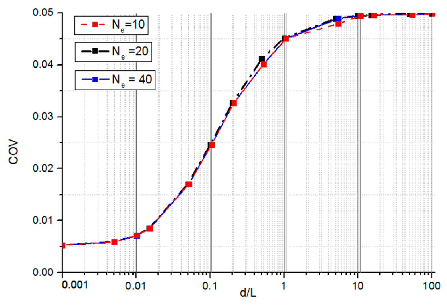
Figure 9 explores the influence of the finite element mesh on the COV of the displacement obtained using the SFEM for beam analysis. Three mesh densities were investigated, with element numbers N_e of 10, 20, and 40. The 2D random field was assigned a standard deviation of 0.05. The correlation length in the x-direction was chosen to be equal to the correlation length in the y-direction. The results reveal a key finding: the COV of the displacement exhibits mesh convergence, indicating independence from the specific finite element mesh employed within the investigated range of element densities. This observation signifies that the chosen SFEM formulation is mesh-insensitive for the given random field characteristics.

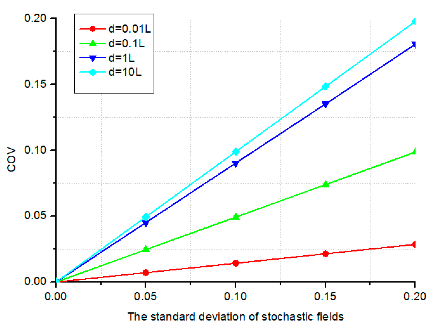
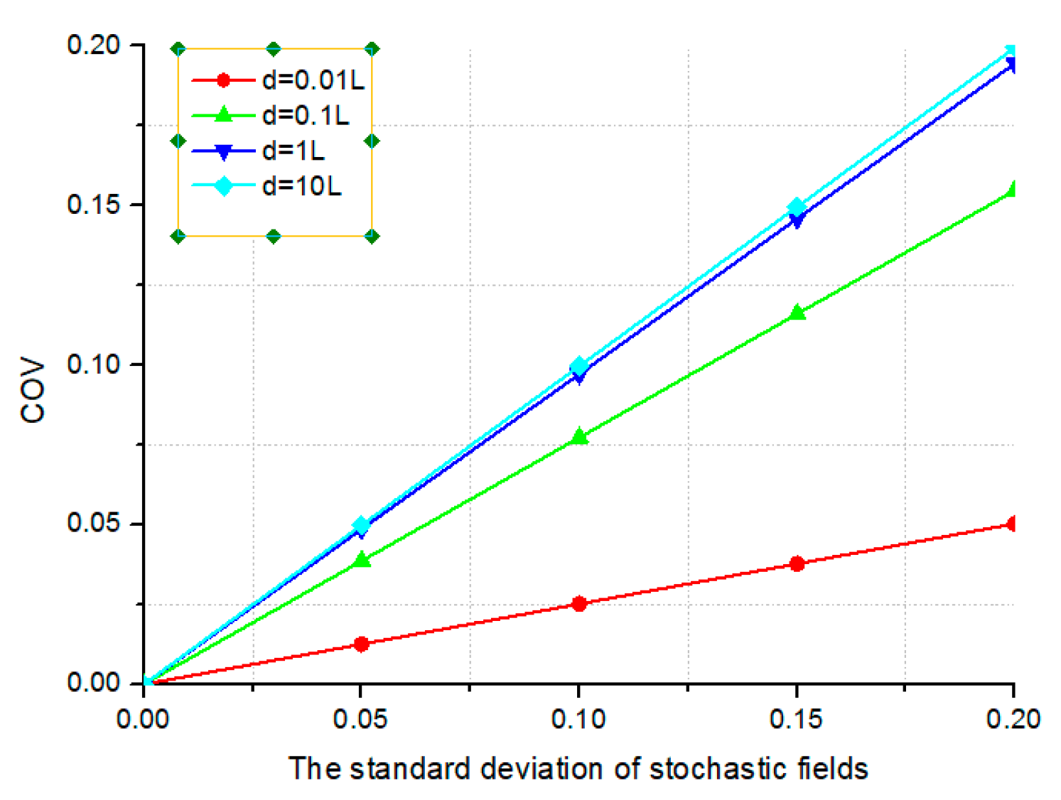
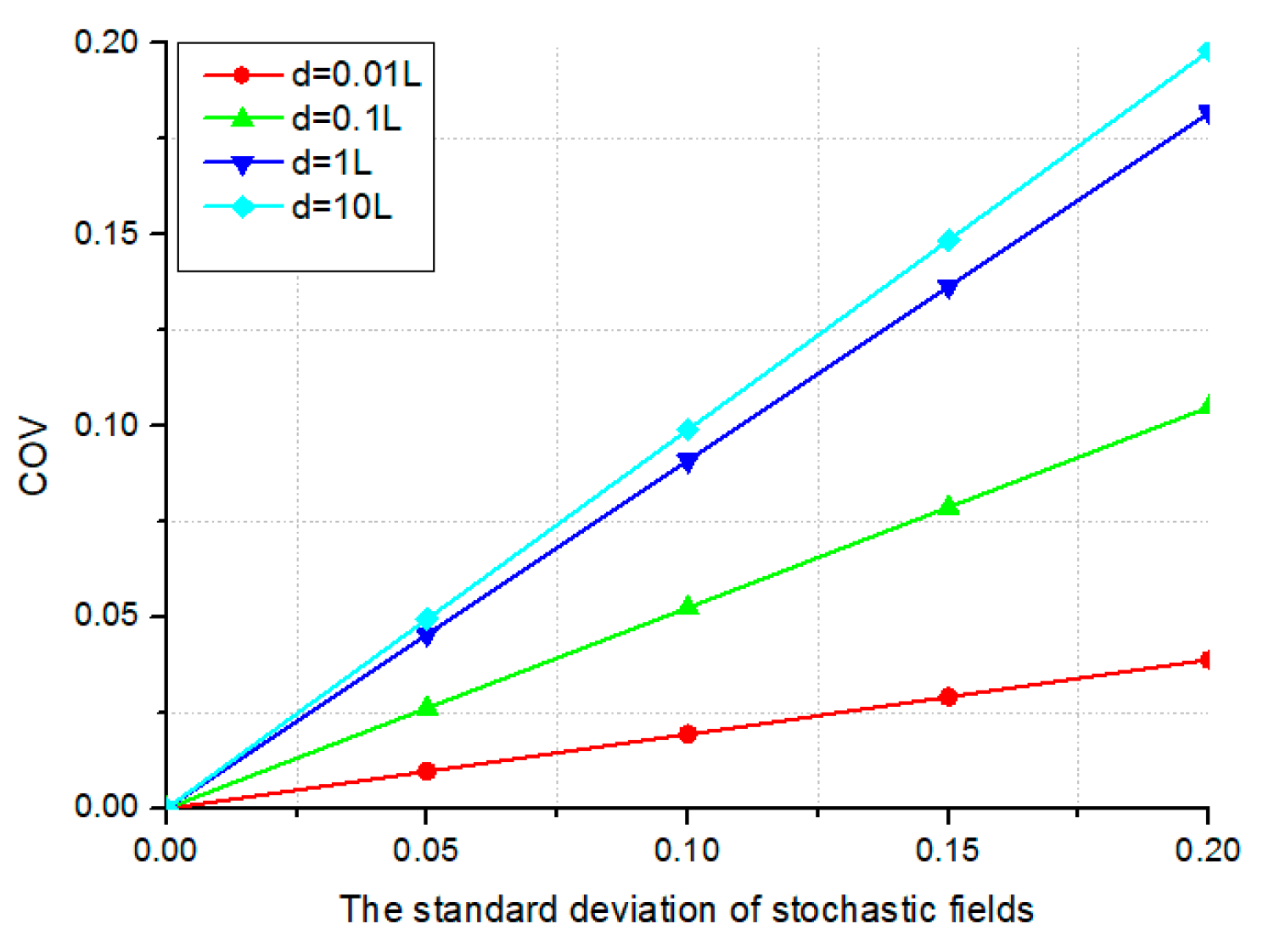
This next section explores the effect of σ_f on the COV of the displacement. A systematic investigation is conducted, varying the standard deviation across a range of values (0, 0.05, 0.10, 0.15, and 0.20) for each of the following correlation lengths: d = 0.01L, 0.1L, L, and 10L (where L represents the beam length). The effects of σ_f on the COV of the displacement for the three distinct relationships between the correlation lengths along the coordinate axes are presented in Figure 10, Figure 11, and Figure 12, respectively. The analysis indicates a nearly linear correlation between σ_f, treated as an input parameter, and the COV of displacement, which characterizes the structure’s stochastic response.

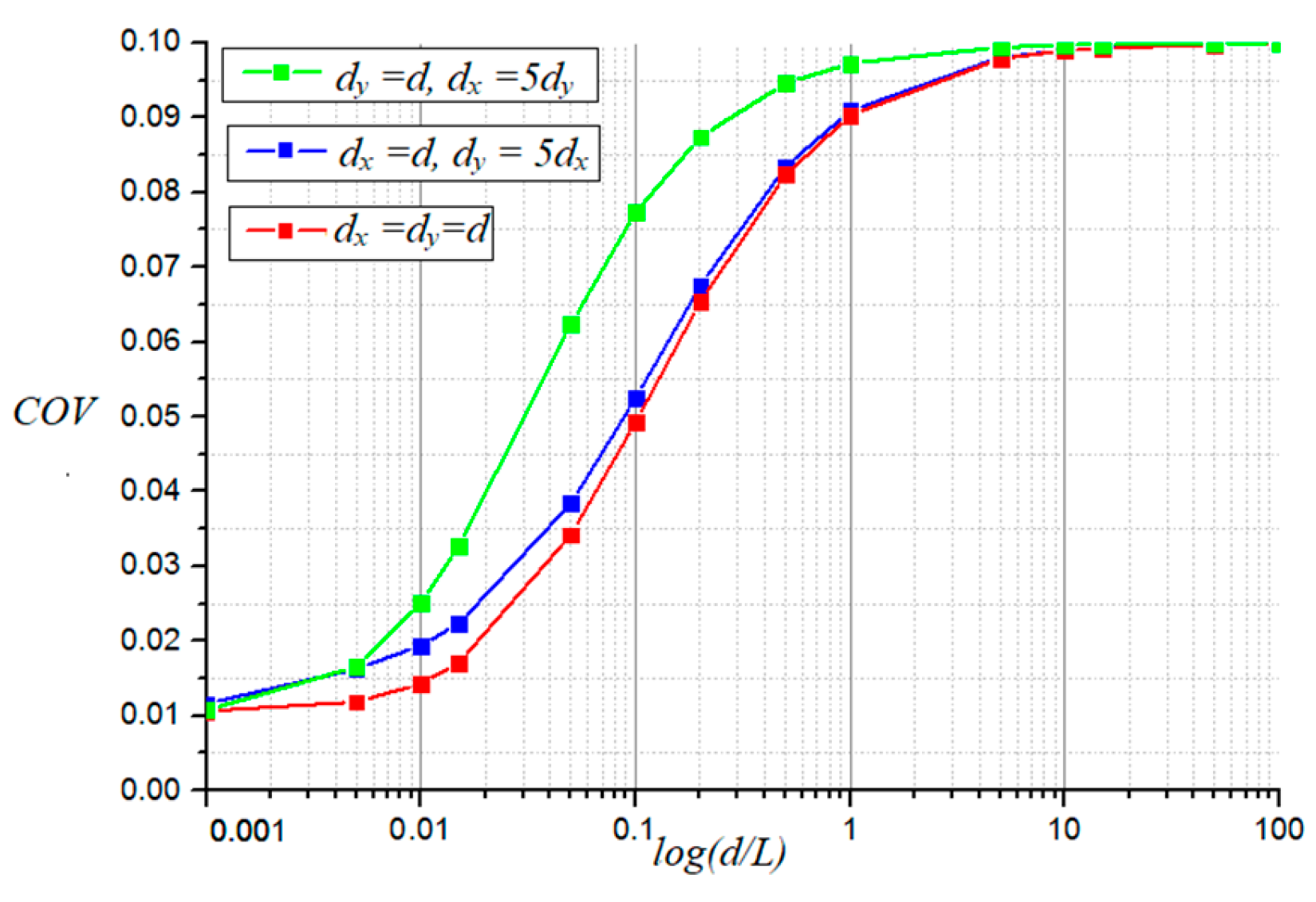
Figure 13 illustrates the effect of the correlation lengths on the COV of displacement. A general trend emerges: the COV increases as correlation lengths along both axes increase. However, the influence of correlation length along the beam’s longitudinal (x) and vertical (y) axes on the COV of displacement exhibits a distinct anisotropy. When the correlation length solely increases along one axis while the other remains constant, the rise in the COV of displacement is significantly more pronounced for the case of growing x-axis correlation length compared to the y-axis, even with identical increments in correlation length values. 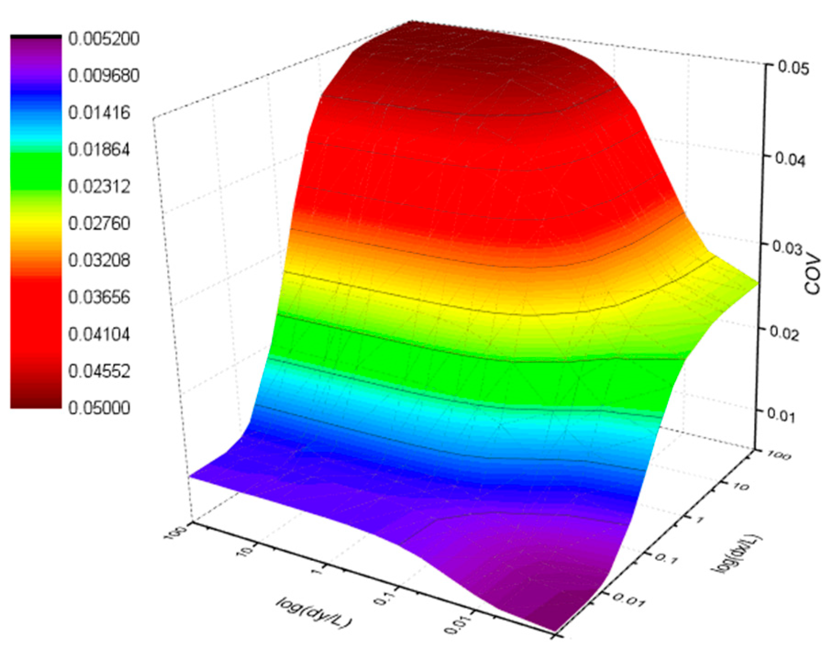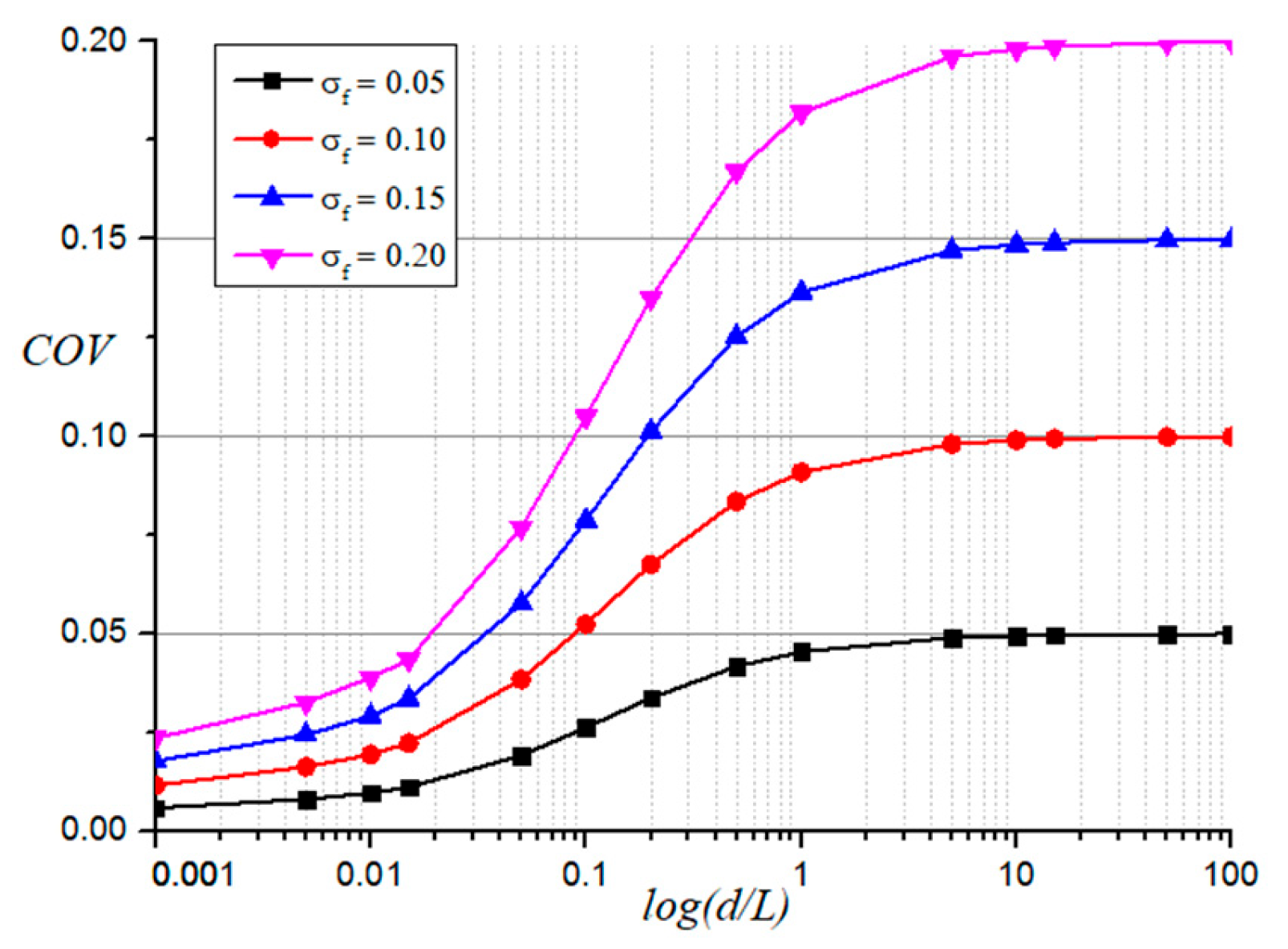Figure 14 further elucidates this anisotropic influence by presenting scenarios where correlation lengths along both axes vary from 0.001L to 100L. The COV of displacement exhibits a direct relationship with correlation length, demonstrating lower values for smaller correlation lengths and progressively higher values for larger ones. Notably, a significant initial increase in the COV of displacement is observed at small correlation length values. As the correlation length increases, the rise in the COV of displacement gradually diminishes, eventually becoming negligible. Interestingly, for considerable correlation lengths approaching infinity, the COV of displacement exhibits a convergence behavior, tending towards the σ_f of a 2D stochastic field. As the correlation length increases, the local fluctuations in the material properties are not effectively averaged out, leading to an increase in the COV of the structural response. In the limiting case where the correlation length becomes very large, the random field over the entire structure approaches homogeneity, causing the COV to converge to a value equivalent to the standard deviation of the input random field. Moreover, the influence of the correlation length in the longitudinal direction of the beam is significantly more pronounced than that in the vertical direction, as the structure is generally more sensitive to variations in material properties along its length.

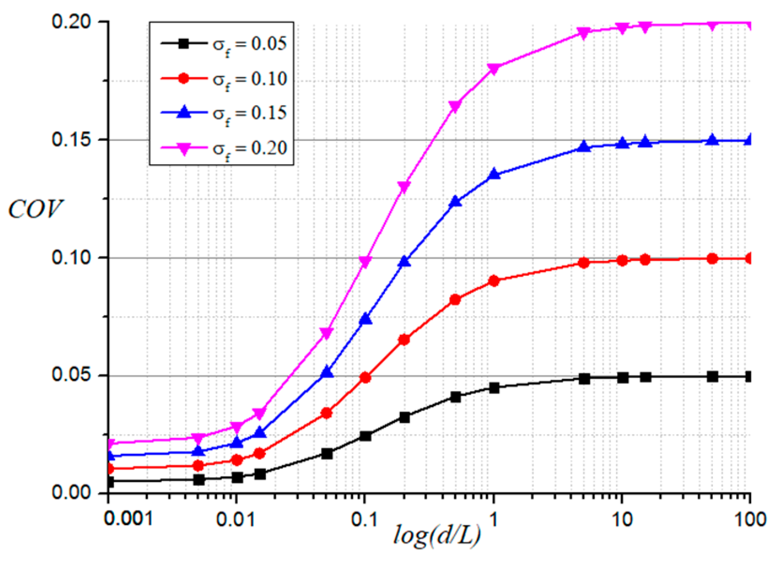
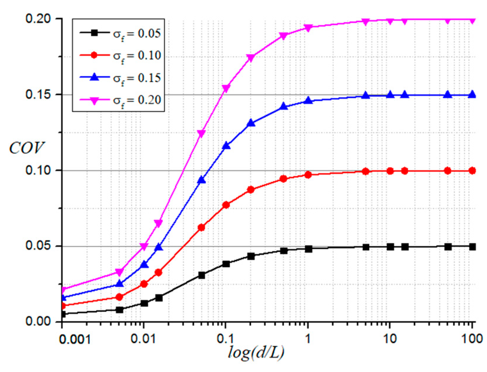
This study delves into the influence of σ_f on the COV of displacement, considering three correlation length relationships along the axes and standard deviation values of 0.05, 0.10, 0.15, and 0.20. The results of this investigation are presented in Figure 15, Figure 16 and Figure 17. The COV of displacement exhibits an increasing trend with the standard deviation. This observation highlights the synergistic effect of correlation lengths along the axes and σ_f on the COV of displacement.

In this study, Young’s modulus is modeled as a homogeneous Gaussian random field due to its mathematical tractability and the well-established theoretical framework associated with spectral representation methods. However, in practice, many materials exhibit non-Gaussian statistical characteristics and spatially non-homogeneous variations.

The extension to non-Gaussian random fields can be achieved using nonlinear transformation techniques. A common approach is to generate an underlying standard Gaussian field and apply an appropriate nonlinear mapping to obtain the desired non-Gaussian distribution, such as log-normal, Weibull, or beta distributions. This transformation preserves the spatial correlation structure while modifying the marginal distribution, allowing the model to more accurately capture the actual material behavior.

Additionally, the Gaussian Regression Method (GRM) or simulation techniques based on experimental data can be employed to construct non-Gaussian fields from observed data. These methods enable the modeling of real-world materials with complex statistical distributions without relying on the Gaussian assumption.

For non-homogeneous fields, they can be modeled by allowing statistical properties (e.g., mean and variance) and correlation structures to vary spatially. This leads to the modeling of non-stationary random fields, which can be represented using advanced spectral methods or modified Karhunen–Loève expansions adapted for non-homogeneous settings. Although computationally more demanding, these models provide a more accurate representation of materials with spatially varying properties, such as functionally graded materials (FGMs) or layered composites.

In future research, incorporating non-Gaussian and non-homogeneous random fields into the stochastic analysis framework could enhance the realism and applicability of the results, particularly for complex materials encountered in engineering practice.

5. Conclusions

This study developed and implemented the SFEM to investigate the static response of beams with a two-dimensional spatially varying elastic modulus. A 2D stationary stochastic field was utilized to capture the material heterogeneity, while the weighted integral method was employed to transform the random field into discrete variables and derive the element stiffness matrices. A first-order perturbation technique was applied to approximate the statistical properties of the nodal displacement, including its mean and covariance matrix. The proposed method’s accuracy and efficiency were assessed through comparisons with MCs, demonstrating a high level of agreement in evaluating the COV of displacement. A sensitivity analysis was performed to examine the impact of the spatial correlation and dispersion of the stochastic elastic modulus field affecting the COV. The findings indicate that the COV increases as these parameters grow, with the most significant variations occurring at small correlation lengths. As the correlation length extends to large values, the COV of displacement converges toward the input variability measure. Furthermore, the study found that the correlation length along the beam’s longitudinal axis exerts a more substantial influence on the COV of displacement compared to the correlation length along the beam’s vertical direction. These findings highlight the importance of accounting for the two-dimensional spatial variability of material properties when analyzing the stochastic response of beam structures.