Analytical Study of Magnetohydrodynamic Casson Fluid Flow over an Inclined Non-Linear Stretching Surface with Chemical Reaction in a Forchheimer Porous Medium

Abstract

This study investigates the steady, two-dimensional boundary layer flow of a Casson fluid over an inclined nonlinear stretching surface embedded within a Forchheimer porous medium. The governing partial differential equations are transformed into a set of ordinary differential equations through similarity transformations. The analysis incorporates the effects of an external uniform magnetic field, gravitational forces, thermal radiation modeled by the Rosseland approximation, and first-order homogeneous chemical reactions. We consider several dimensionless parameters, including the Casson fluid parameter, magnetic parameter, Darcy and Forchheimer numbers, Prandtl and Schmidt numbers, and the Eckert number to characterize the flow, heat, and mass transfer phenomena. Analytical solutions for the velocity, temperature, and concentration profiles are derived under simplifying assumptions, and expressions for critical physical quantities such as the skin friction coefficient, Nusselt number, and Sherwood number are obtained.

1. Introduction

The study of the magnetohydrodynamic (MHD) flow of non-Newtonian fluids over inclined surfaces in porous media is of importance due to its applications in engineering and geophysical processes, such as petroleum extraction, geothermal energy systems, and chemical reactors [1,2,3]. Casson fluids, characterized by their yield stress behavior, are particularly relevant in modeling materials like blood, honey, and certain industrial suspensions [4,5]. Recent advancements have explored the complexities introduced by anisotropic permeability and non-linear drag forces within such mediums. For instance, Aich et al. [6] investigated forced convective heat transport in a rectangular porous channel with anisotropic permeability using a non-linear Brinkman–Forchheimer extended Darcy’s model. Their computational study showed the effect of anisotropic parameters in enhancing heat transmission, demonstrating an over 13% increase in heat transfer rates compared to isotropic scenarios. Moreover, Zhang and Sun [7] employed a coupled Lattice Boltzmann approach to model gas flow across different scales within shale reservoirs. Their work emphasized the robustness and efficiency of mesoscopic methods in handling multi-scale interactions, which is relevant for accurate predictions in complex porous structures. The generation of magnetic fields through fluid motion in conducting fluids has been a subject of intense research. Chertovskih et al. [8] numerically studied magnetic field generation in three-dimensional Rayleigh–Bénard convection, revealing the dynamics of hyperchaos and intermittency in magnetic energy.

In this work, we consider the steady, two-dimensional boundary layer flow of a Casson fluid over an inclined nonlinear stretching surface embedded in a Forchheimer porous medium. The flow domain $\Omega \subset {\mathbb{R}}^2$ is defined such that the x-axis lies along the inclined surface, and the y-axis is normal to it. The inclination angle of the surface is $\theta$ with respect to the horizontal axis. A schematic diagram of the physical model is depicted in Figure 1.

An external uniform magnetic field $B_0$ is applied perpendicular to the surface along the y-direction. The fluid is electrically conducting, and flows under the influence of this magnetic field. Gravity acts downward, making an angle $\theta$ with the x-axis, consistent with the inclination of the surface.

The stretching surface has a velocity $U_w\left(x\right)$, temperature $T_w\left(x\right)$, and concentration $C_w\left(x\right)$ that are prescribed functions of the position along the surface. The ambient temperature and concentration far from the surface are $T_{\infty }$ and $C_{\infty }$, respectively.

The following assumptions are made in the formulation of the problem:

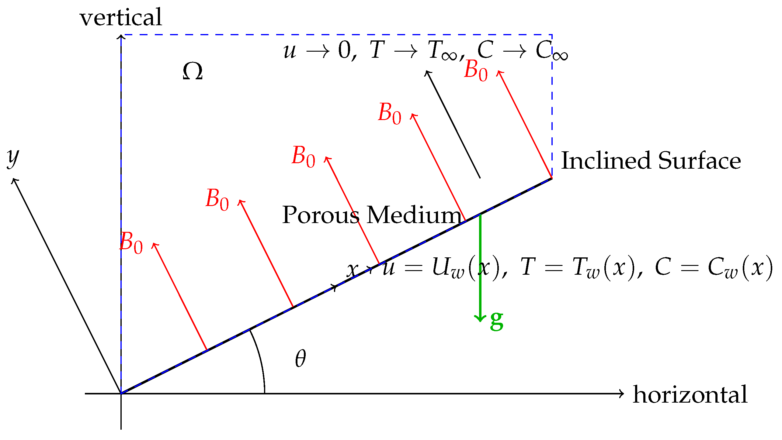
• The fluid is an incompressible Casson fluid, exhibiting non-Newtonian behavior characterized by the Casson model.
• The flow is steady, two-dimensional, and laminar.
• The boundary layer approximations are applicable, meaning that variations in the flow properties in the y-direction are much more significant than those in the x-direction.
• The induced magnetic field due to the fluid motion is negligible compared to the applied magnetic field (low magnetic Reynolds number assumption) [9].
• The pressure gradient in the y-direction is negligible within the boundary layer.
• The fluid properties are constant except for the density variations in the buoyancy term (Boussinesq approximation).
• The radiative heat flux is modeled using the Rosseland approximation [4,10].
• The porous medium is homogeneous and isotropic, and the Forchheimer extension accounts for inertial effects at higher flow velocities.
• Chemical reactions are homogeneous and of first order.

Under the above assumptions, the governing equations for the problem are as follows.

Continuity equation:

$${\displaystyle \frac{\partial u}{\partial x}}+{\displaystyle \frac{\partial v}{\partial y}}=0.$$

(1)

Momentum equation in the x-direction:

$$\rho \left(u{\displaystyle \frac{\partial u}{\partial x}}+v{\displaystyle \frac{\partial u}{\partial y}}\right)=-{\displaystyle \frac{\partial p}{\partial x}}+{\mu }_B\left(1+{\displaystyle \frac{1}{\beta }}\right){\displaystyle \frac{{\partial }^{2}u}{\partial y^2}}-\sigma B_0^{2}u-{\displaystyle \frac{{\mu }_B\left(1+{\displaystyle \frac{1}{\beta }}\right)}{K}}u-{\beta }^{\ast }\rho u^2+\rho gsin\theta .$$

(2)

Momentum equation in the y-direction: under the boundary layer approximation, the momentum equation in the y-direction simplifies to

$$0=-{\displaystyle \frac{\partial p}{\partial y}}+\rho gcos\theta .$$

(3)

Since the pressure gradient in the y-direction is negligible within the boundary layer, we assume ${\displaystyle \frac{\partial p}{\partial y}}\approx 0$. Therefore, the pressure p is a function of x only.

Energy equation:

$$\begin{array}{cc}\hfill \rho c_p\left(u{\displaystyle \frac{\partial T}{\partial x}}+v{\displaystyle \frac{\partial T}{\partial y}}\right)& =k{\displaystyle \frac{{\partial }^{2}T}{\partial y^2}}-{\displaystyle \frac{\partial q_r}{\partial y}}+Q(T-T_{\infty })\hfill \\ \hfill & +{\mu }_B\left(1+{\displaystyle \frac{1}{\beta }}\right){\left({\displaystyle \frac{\partial u}{\partial y}}\right)}^2+\sigma B_0^2{u}^2+{\displaystyle \frac{{\mu }_B\left(1+{\displaystyle \frac{1}{\beta }}\right)}{K}}{u}^2+{\beta }^{\ast }\rho u^3.\hfill \end{array}$$

(4)

Species concentration equation:

$$u{\displaystyle \frac{\partial C}{\partial x}}+v{\displaystyle \frac{\partial C}{\partial y}}=D{\displaystyle \frac{{\partial }^{2}C}{\partial y^2}}-k_r(C-C_{\infty }).$$

(5)

Radiative heat flux: the radiative heat flux $q_r$ is modeled using the Rosseland approximation,

$$q_r=-{\displaystyle \frac{4{\sigma }^{\ast }}{3k^{\ast }}}{\displaystyle \frac{\partial T^4}{\partial y}},$$

(6)

where ${\sigma }^{\ast }$ is the Stefan–Boltzmann constant, and $k^{\ast }$ is the mean absorption coefficient.

1.1. Boundary Conditions

At the wall ($y=0$),

$$u=U_w\left(x\right),v=0,T=T_w\left(x\right),C=C_w\left(x\right).$$

(7)

As $y\to \infty$,

$$u\to 0,T\to T_{\infty },C\to C_{\infty }.$$

(8)

1.2. Definitions of Parameters

• $\rho$ is the fluid density.
• p is the pressure.
• ${\mu }_B$ is the plastic dynamic viscosity of the Casson fluid.
• $\beta$ is the Casson fluid parameter, related to the yield stress ${\tau }_y$ by $\beta ={\displaystyle \frac{{\mu }_B\sqrt{2\pi }}{{\tau }_y}}$ [11,12].
• $\sigma$ is the electrical conductivity of the fluid.
• $B_0$ is the strength of the applied magnetic field.
• K is the permeability of the porous medium.
• ${\beta }^{\ast }$ is the Forchheimer inertial coefficient, representing the non-linear drag in the porous medium [13].
• g is the acceleration due to gravity.
• $\theta$ is the inclination angle of the surface.
• $c_p$ is the specific heat at constant pressure.
• k is the thermal conductivity.
• Q is the volumetric heat generation ($Q>0$) or absorption ($Q<0$) coefficient.
• $T_{\infty }$ is the ambient temperature.
• D is the mass diffusivity.
• $k_r$ is the rate constant of the chemical reaction.
• $C_{\infty }$ is the ambient concentration.
• $U_w\left(x\right)$, $T_w\left(x\right)$, and $C_w\left(x\right)$ are the prescribed velocity, temperature, and concentration at the wall.

2. Discussion of Assumptions and Simplifications

2.1. Boundary Layer Approximations

In the boundary layer theory [14,15], the flow is predominantly in the x-direction, and variations in the y-direction are much more significant than those in the x-direction. Therefore,

• The term ${\displaystyle \frac{{\partial }^{2}u}{\partial x^2}}$ is negligible compared to ${\displaystyle \frac{{\partial }^{2}u}{\partial y^2}}$ in the momentum equation.
• The pressure gradient in the y-direction is negligible, i.e., ${\displaystyle \frac{\partial p}{\partial y}}\approx 0$.
• The flow velocity component v in the y-direction is much smaller than u and is determined from the continuity equation.

2.2. Low Magnetic Reynolds Number

The magnetic Reynolds number $R_m$ is assumed to be small ($R_m\ll 1$), which implies that the induced magnetic field due to the fluid motion is negligible compared to the applied magnetic field $B_0$ [9]. Therefore, the magnetic field is considered to be constant, and the Lorentz force term $-\sigma B_0^{2}u$ in the momentum equation accounts for the magnetic effects.

2.3. Forchheimer Porous Medium

The inclusion of the Forchheimer inertial coefficient ${\beta }^{\ast }$ accounts for the non-linear inertial effects in the porous medium at higher flow velocities [13]. The modified Darcy–Forchheimer term $-{\displaystyle \frac{{\mu }_B\left(1+{\displaystyle \frac{1}{\beta }}\right)}{K}}u-{\beta }^{\ast }\rho u^2$ represents the resistance due to the porous medium.

2.4. Energy Equation Adaptation

The energy Equation (4) includes additional terms to account for the following:

• Viscous dissipation: the term ${\mu }_B\left(1+{\displaystyle \frac{1}{\beta }}\right){\left({\displaystyle \frac{\partial u}{\partial y}}\right)}^2$ represents the viscous dissipation due to the Casson fluid’s rheological properties.
• Joule heating: the term $\sigma B_0^2{u}^2$ accounts for the heat generated due to the interaction between the magnetic field and the electrically conducting fluid.
• Porous medium dissipation: the terms ${\displaystyle \frac{{\mu }_B\left(1+{\displaystyle \frac{1}{\beta }}\right)}{K}}{u}^2$ and ${\beta }^{\ast }\rho u^3$ represent the energy dissipation due to the porous medium’s resistance.

These terms are significant in the energy balance, and contribute to the thermal energy of the system.

3. Formulated Problem

To simplify the analysis and reduce the governing partial differential equations to ordinary differential equations, we introduce the following similarity variables:

$$\begin{array}{cc}\hfill & \eta =y{\left({\displaystyle \frac{U_0}{\nu x^m}}\right)}^{1/2},\hfill \end{array}$$

(9)

$$\begin{array}{cc}\hfill & \theta \left(\eta \right)={\displaystyle \frac{T-T_{\infty }}{T_w\left(x\right)-T_{\infty }}},\varphi \left(\eta \right)={\displaystyle \frac{C-C_{\infty }}{C_w\left(x\right)-C_{\infty }}},\hfill \end{array}$$

(10)

where

• $U_0$ is a characteristic velocity.
• $\nu ={\displaystyle \frac{{\mu }_B}{\rho }}$ is the kinematic viscosity.
• m is a parameter indicating the nonlinearity of the stretching surface. In case of a linear stretching, $m=1$, and we will consider this case unless otherwise specified.
• $f\left(\eta \right)$, $\theta \left(\eta \right)$, and $\varphi \left(\eta \right)$ are dimensionless similarity functions to be determined [1,16].

Substituting the similarity variables (9) and (10) into the governing Equations (2)–(5), and using the definitions of the dimensionless parameters, we obtain the following ordinary differential equations.

3.1. Dimensionless Momentum Equation

To facilitate the conversion of the equations into its dimensionless forms, we introduce the stream function $\psi (x,y)$ such that:

$$\begin{array}{c}\hfill u={\displaystyle \frac{\partial \psi }{\partial y}},v=-{\displaystyle \frac{\partial \psi }{\partial x}}.\end{array}$$

(11)

Considering $m=1$ in the similarity transformation (9), let the stream function be:

$$\psi ={\left(\nu U_{0}x\right)}^{1/2}f\left(\eta \right).$$

(12)

Computing u and v:

$$\begin{array}{cc}\hfill u& ={\displaystyle \frac{\partial \psi }{\partial y}}={\left(\nu U_{0}x\right)}^{1/2}{f}^{\prime }\left(\eta \right){\displaystyle \frac{\partial \eta }{\partial y}},\hfill \end{array}$$

(13)

$$\begin{array}{cc}\hfill {\displaystyle \frac{\partial \eta }{\partial y}}& ={\left({\displaystyle \frac{U_0}{\nu x}}\right)}^{1/2},\hfill \end{array}$$

(14)

$$\begin{array}{cc}\hfill \Rightarrow u& =U_0{f}^{\prime }\left(\eta \right).\hfill \end{array}$$

(15)

$$\begin{array}{cc}\hfill v& =-{\displaystyle \frac{\partial \psi }{\partial x}}=-{\displaystyle \frac{1}{2}}{\left({\displaystyle \frac{\nu U_0}{x}}\right)}^{1/2}f\left(\eta \right)-{\left(\nu U_{0}x\right)}^{1/2}{f}^{\prime }\left(\eta \right)\left(-{\displaystyle \frac{1}{2}}{\displaystyle \frac{\eta }{x}}\right),\hfill \end{array}$$

(16)

$$\begin{array}{cc}\hfill \Rightarrow v& =-{\displaystyle \frac{1}{2}}{\left({\displaystyle \frac{\nu U_0}{x}}\right)}^{1/2}\left(f\left(\eta \right)-\eta f^{\prime }\left(\eta \right)\right).\hfill \end{array}$$

(17)

Then, from the momentum Equation (2), we obtain

$$\left(1+{\displaystyle \frac{1}{\beta }}\right)f^{‴}\left(\eta \right)+{\displaystyle \frac{1}{2}}f{f}^{″}\left(\eta \right)-M{f}^{\prime }\left(\eta \right)-\left(1+{\displaystyle \frac{1}{\beta }}\right){\displaystyle \frac{1}{\mathrm{Da}}}{f}^{\prime }\left(\eta \right)-F{\left(f^{\prime }\left(\eta \right)\right)}^2+Gsin\alpha =0.$$

(18)

where

• $f^{\prime }={\displaystyle \frac{df}{d\eta }}$, $f^{″}={\displaystyle \frac{d^{2}f}{d{\eta }^2}}$, $f^{‴}={\displaystyle \frac{d^{3}f}{d{\eta }^3}}$.
• $\beta ={\displaystyle \frac{{\mu }_B\sqrt{2\pi }}{{\tau }_y}}$ is the Casson fluid parameter.
• $M={\displaystyle \frac{\sigma B_0^2}{\rho U_0}}$ is the magnetic parameter.
• $\mathrm{Da}={\displaystyle \frac{K{U}_0}{\nu x_0}}$ is the Darcy number.
• $F={\beta }^{\ast }{x}_0$ is the Forchheimer parameter.
• $G={\displaystyle \frac{g{x}_0}{U_0^2}}$ is the modified Grashof number.
• $\alpha$ is the inclination angle of the surface.
• $\nu ={\displaystyle \frac{{\mu }_B}{\rho }}$ is the kinematic viscosity.
• ${\beta }^{\ast }$ is the Forchheimer inertial coefficient.
• $x_0$ is the reference length.

3.2. Dimensionless Energy Equation

From the energy Equation (4), we obtain

$$\begin{array}{c}\hfill (1+N_r){\theta }^{″}+Prf{\theta }^{\prime }+PrN\theta +Pr{E}_c\left[\left(1+{\displaystyle \frac{1}{\beta }}\right){\left(f^{″}\right)}^2+M{\left(f^{\prime }\right)}^2+{\displaystyle \frac{\left(1+{\displaystyle \frac{1}{\beta }}\right)}{\mathrm{Da}}}{\left(f^{\prime }\right)}^2+F{\left(f^{\prime }\right)}^3\right]=0,\end{array}$$

(19)

To obtain this last expressed we consider smooth variation of $T_w$ with x, and the linearization of the radiation term using the Rosseland approximation. Each term in the dimensionless energy equation has the following significance:

• $(1+N_r){\theta }^{″}$: represents the combined effect of thermal conduction and thermal radiation on heat diffusion within the boundary layer.

  –

  The radiation parameter $N_r={\displaystyle \frac{16{\sigma }^{\ast }{T}_{\infty }^3}{3k^{\ast }k}}$ enhances the effective thermal diffusivity due to radiative heat transfer.

  –

  Derived by combining Fourier’s law of heat conduction with the Rosseland approximation for radiative heat flux, leading to an effective thermal conductivity $k_{\mathrm{eff}}=k(1+N_r)$.

• $Prf{\theta }^{\prime }$: accounts for convective heat transfer due to fluid motion along the stretching surface.

  –

  Pr is the Prandtl number, indicating the ratio of momentum diffusivity to thermal diffusivity.

  –

  f is the dimensionless stream function related to the velocity profile.

  –

  ${\theta }^{\prime }$ is the first derivative of the dimensionless temperature with respect to $\eta$.

• $PrN\theta$: represents the effect of volumetric heat generation ($N>0$) or absorption ($N<0$) within the fluid.

  –

  N is the dimensionless heat generation or absorption parameter: $N={\displaystyle \frac{Q}{\rho c_p{U}_0}}$.

  –

  $\theta$ is the dimensionless temperature.

• $Pr{E}_c\left(1+{\displaystyle \frac{1}{\beta }}\right){\left(f^{″}\right)}^2$: corresponds to viscous dissipation within the Casson fluid.

  –

  $\beta$ is the Casson fluid parameter, modifying the viscous effects due to the non-Newtonian behavior of the fluid.

  –

  $f^{″}$ is the second derivative of the dimensionless stream function.

  –

  $E_c$ is the Eckert number, quantifying the ratio of kinetic energy to enthalpy difference: $E_c={\displaystyle \frac{U_0^2}{c_p(T_w-T_{\infty })}}$.

• $Pr{E}_{c}M{\left(f^{\prime }\right)}^2$: accounts for Joule heating due to the interaction between the applied magnetic field and the electrically conducting fluid.

  –

  M is the magnetic parameter, representing the strength of the magnetic field effects.

  –

  $f^{\prime }$ is the first derivative of the dimensionless stream function.

• $Pr{E}_c{\displaystyle \frac{\left(1+{\displaystyle \frac{1}{\beta }}\right)}{Da}}{\left(f^{\prime }\right)}^2$: represents energy dissipation due to the resistance of the porous medium.

  –

  Da is the Darcy number, characterizing the permeability of the porous medium.

  –

  The term reflects the additional frictional heating due to the flow through the porous structure.

• $Pr{E}_{c}F{\left(f^{\prime }\right)}^3$: captures additional energy dissipation due to inertial effects within the porous medium.

  –

  F is the Forchheimer parameter, accounting for nonlinear drag effects at higher velocities.

  –

  The cubic dependence on $f^{\prime }$ indicates the nonlinear nature of these inertial effects.

3.3. Dimensionless Concentration Equation

From the concentration Equation (5), we obtain

$${\varphi }^{″}+\mathrm{Sc}f{\varphi }^{\prime }-\mathrm{Sc}{K}_r\varphi =0,$$

(20)

where

• ${\varphi }^{\prime }={\displaystyle \frac{d\varphi }{d\eta }}$, ${\varphi }^{″}={\displaystyle \frac{d^2\varphi }{d{\eta }^2}}$.
• $\mathrm{Sc}={\displaystyle \frac{\nu }{D}}$ is the Schmidt number.
• $K_r={\displaystyle \frac{k_r{x}_0^{(1-m)/2}}{U_0^{1/2}{\nu }^{1/2}}}$ is the dimensionless chemical reaction rate parameter which is independent of the characteristic length $x_0$ for $m=1$.

Each term in the dimensionless concentration equation has specific physical significance:

• ${\varphi }^{″}$: represents the diffusion of concentration due to molecular (mass) diffusion.
• $\mathrm{Sc}f{\varphi }^{\prime }$: considers the convective transport of concentration driven by fluid motion. Here, $\mathrm{Sc}$ is the Schmidt number, f is the dimensionless stream function, and ${\varphi }^{\prime }$ is the concentration gradient.
• $-\mathrm{Sc}{K}_r\varphi$: Accounts for the first-order homogeneous chemical reaction affecting the concentration. The parameter $K_r$ quantifies the reaction rate’s influence relative to convection.

3.4. Boundary Conditions

The boundary conditions transform to

$$\begin{array}{cc}\hfill & f\left(0\right)=0,f^{\prime }\left(0\right)=1,\theta \left(0\right)=1,\varphi \left(0\right)=1,\hfill \end{array}$$

(21)

$$\begin{array}{cc}\hfill & f^{\prime }(\infty )\to 0,\theta (\infty )\to 0,\varphi (\infty )\to 0.\hfill \end{array}$$

(22)

4. Mathematical Analysis

In this section, we focus on deriving expressions for important physical quantities such as the skin friction coefficient, Nusselt number, and Sherwood number, based on the solutions of the dimensionless ordinary differential equations obtained earlier.

4.1. Analytical Resolution of the Skin Friction Coefficient

We recall that the skin friction coefficient $C_f$ is a dimensionless quantity representing the shear stress at the wall normalized by the dynamic pressure. It is defined as

$$C_f={\displaystyle \frac{{\tau }_w}{{\displaystyle \frac{1}{2}}\rho U_w^2}},$$

(23)

where ${\tau }_w$ is the shear stress at the wall, given by

$${\tau }_w={\mu }_{\mathrm{eff}}{\left({\displaystyle \frac{\partial u}{\partial y}}\right)}_{y=0}.$$

(24)

The effective dynamic viscosity ${\mu }_{\mathrm{eff}}$ is

$${\mu }_{\mathrm{eff}}={\mu }_B\left(1+{\displaystyle \frac{1}{\beta }}\right),$$

(25)

where ${\mu }_B$ is the plastic dynamic viscosity of the Casson fluid, and $\beta$ is the Casson fluid parameter.

Using the similarity transformation $u=U_w{f}^{\prime }\left(\eta \right)$ and $U_w=U_0{x}^m$, and noting that

$${\displaystyle \frac{\partial u}{\partial y}}=U_w{f}^{″}\left(\eta \right){\displaystyle \frac{\partial \eta }{\partial y}},$$

(26)

and since

$$\eta =y{\left({\displaystyle \frac{U_0}{\nu x^m}}\right)}^{1/2}\Rightarrow {\displaystyle \frac{\partial \eta }{\partial y}}={\left({\displaystyle \frac{U_0}{\nu x^m}}\right)}^{1/2},$$

(27)

we have

$${\displaystyle \frac{\partial u}{\partial y}}=U_w{f}^{″}\left(\eta \right){\left({\displaystyle \frac{U_0}{\nu x^m}}\right)}^{1/2}.$$

(28)

Evaluating at $y=0$ (where $\eta =0$):

$${\left({\displaystyle \frac{\partial u}{\partial y}}\right)}_{y=0}=U_w{\left({\displaystyle \frac{U_0}{\nu x^m}}\right)}^{1/2}{f}^{″}\left(0\right).$$

(29)

Substituting this into the expression for ${\tau }_w$:

$${\tau }_w={\mu }_B\left(1+{\displaystyle \frac{1}{\beta }}\right)U_w{\left({\displaystyle \frac{U_0}{\nu x^m}}\right)}^{1/2}{f}^{″}\left(0\right).$$

(30)

Substituting ${\tau }_w$ into Equation (23), we obtain

$$\begin{array}{cc}\hfill C_f& ={\displaystyle \frac{2{\tau }_w}{\rho U_w^2}}\hfill \\ \hfill & ={\displaystyle \frac{2{\mu }_B\left(1+{\displaystyle \frac{1}{\beta }}\right)U_w{\left({\displaystyle \frac{U_0}{\nu x^m}}\right)}^{1/2}{f}^{″}\left(0\right)}{\rho U_w^2}}\hfill \\ \hfill & ={\displaystyle \frac{2{\mu }_B\left(1+{\displaystyle \frac{1}{\beta }}\right)f^{″}\left(0\right)}{\rho U_w}}{\left({\displaystyle \frac{U_0}{\nu x^m}}\right)}^{1/2}.\hfill \end{array}$$

(31)

Since ${\mu }_B=\rho \nu$, we have

$$\begin{array}{cc}\hfill C_f& ={\displaystyle \frac{2\rho \nu \left(1+{\displaystyle \frac{1}{\beta }}\right)f^{″}\left(0\right)}{\rho U_w}}{\left({\displaystyle \frac{U_0}{\nu x^m}}\right)}^{1/2}\hfill \\ \hfill & =2\nu \left(1+{\displaystyle \frac{1}{\beta }}\right){\displaystyle \frac{f^{″}\left(0\right)}{U_w}}{\left({\displaystyle \frac{U_0}{\nu x^m}}\right)}^{1/2}.\hfill \end{array}$$

(32)

Simplifying the terms:

$$\begin{array}{cc}\hfill C_f& =2\left(1+{\displaystyle \frac{1}{\beta }}\right)f^{″}\left(0\right){\displaystyle \frac{{\nu }^{1-1/2}}{U_w}}{\displaystyle \frac{U_0^{1/2}}{x^{m/2}}}\hfill \\ \hfill & =2\left(1+{\displaystyle \frac{1}{\beta }}\right)f^{″}\left(0\right){\displaystyle \frac{{\nu }^{1/2}}{U_w}}{\displaystyle \frac{U_0^{1/2}}{x^{m/2}}}.\hfill \end{array}$$

(33)

Since $U_w=U_0{x}^m$, we have

$${\displaystyle \frac{1}{U_w}}={\displaystyle \frac{1}{U_0{x}^m}}.$$

(34)

Substituting back, we get

$$\begin{array}{cc}\hfill C_f& =2\left(1+{\displaystyle \frac{1}{\beta }}\right)f^{″}\left(0\right){\displaystyle \frac{{\nu }^{1/2}{U}_0^{1/2}}{U_0{x}^m{x}^{m/2}}}\hfill \\ \hfill & =2\left(1+{\displaystyle \frac{1}{\beta }}\right)f^{″}\left(0\right){\displaystyle \frac{{\nu }^{1/2}}{U_0^{1/2}{x}^{\left(3m\right)/2}}}.\hfill \end{array}$$

(35)

Solving for ${\displaystyle \frac{{\nu }^{1/2}}{U_0^{1/2}}}$:

$${\displaystyle \frac{{\nu }^{1/2}}{U_0^{1/2}}}={\displaystyle \frac{x^{(m+1)/2}}{R{e}_x^{1/2}}}.$$

(36)

Substituting back into $C_f$:

$$\begin{array}{cc}\hfill C_f& =2\left(1+{\displaystyle \frac{1}{\beta }}\right)f^{″}\left(0\right){\displaystyle \frac{1}{x^{\left(3m\right)/2}}}·{\displaystyle \frac{x^{(m+1)/2}}{R{e}_x^{1/2}}}\hfill \\ \hfill & =2\left(1+{\displaystyle \frac{1}{\beta }}\right)f^{″}\left(0\right){\displaystyle \frac{x^{(m+1)/2-\left(3m\right)/2}}{R{e}_x^{1/2}}}\hfill \\ \hfill & =2\left(1+{\displaystyle \frac{1}{\beta }}\right)f^{″}\left(0\right)x^{-m}R{e}_x^{-1/2}.\hfill \end{array}$$

(37)

For $m=1$:

$$\begin{array}{cc}\hfill C_f& =2\left(1+{\displaystyle \frac{1}{\beta }}\right)f^{″}\left(0\right)x^{-1}R{e}_x^{-1/2}.\hfill \end{array}$$

(38)

Multiplying both sides by x:

$$C_{f}x=2\left(1+{\displaystyle \frac{1}{\beta }}\right)f^{″}\left(0\right)R{e}_x^{-1/2}.$$

(39)

Alternatively, expressing $C_{f}R{e}_x^{1/2}x$:

$$\begin{array}{cc}\hfill C_{f}R{e}_x^{1/2}x& =2\left(1+{\displaystyle \frac{1}{\beta }}\right)f^{″}\left(0\right).\hfill \end{array}$$

(40)

This shows that $C_{f}R{e}_x^{1/2}x$ is constant (independent of x) when $m=1$.

Parametric Discussion of the Skin Friction Coefficient

As $\beta$ decreases, the term $\left(1+{\displaystyle \frac{1}{\beta }}\right)$ increases, leading to a higher skin friction coefficient $C_f$. Physically, this is because a lower $\beta$ corresponds to a fluid with higher yield stress, increasing resistance to shear and, thus, increasing the wall shear stress ${\tau }_w$.

Similarly, parameters that affect $f^{″}\left(0\right)$ will influence the skin friction coefficient. An increase in the magnetic parameter M or a decrease in the Darcy number Da will generally increase $f^{″}\left(0\right)$ due to increased resistance to the flow, thus increasing $C_{f}xR{e}_x^{1/2}$.

4.2. Analytical Resolution of the Nusselt Number

The Nusselt number $N{u}_x$ characterizes the convective heat transfer at the surface and is defined as

$$N{u}_x={\displaystyle \frac{x{q}_w}{k(T_w-T_{\infty })}},$$

(41)

where $q_w$ is the total heat flux at the wall, including both conduction and thermal radiation effects:

$$q_w=-k_{\mathrm{eff}}{\left({\displaystyle \frac{\partial T}{\partial y}}\right)}_{y=0},$$

(42)

and $k_{\mathrm{eff}}$ is the effective thermal conductivity given by

$$k_{\mathrm{eff}}=k(1+N_r),$$

(43)

with $N_r$ being the radiation parameter as we introduced earlier.

Using the similarity transformation for temperature, we have

$$T=T_{\infty }+(T_w-T_{\infty })\theta \left(\eta \right).$$

(44)

Therefore, the temperature gradient at the wall is

$${\left({\displaystyle \frac{\partial T}{\partial y}}\right)}_{y=0}=(T_w-T_{\infty }){\theta }^{\prime }\left(0\right){\displaystyle \frac{\partial \eta }{\partial y}}.$$

(45)

Substituting back, we find

$${\left({\displaystyle \frac{\partial T}{\partial y}}\right)}_{y=0}=(T_w-T_{\infty }){\theta }^{\prime }\left(0\right){\left({\displaystyle \frac{U_0}{\nu x^m}}\right)}^{1/2}.$$

(46)

Therefore, the total heat flux at the wall is

$$q_w=-k_{\mathrm{eff}}(T_w-T_{\infty }){\theta }^{\prime }\left(0\right){\left({\displaystyle \frac{U_0}{\nu x^m}}\right)}^{1/2}.$$

(47)

Substituting $q_w$ into Equation (41), we obtain

$$\begin{array}{cc}\hfill N{u}_x& ={\displaystyle \frac{x\left[-k_{\mathrm{eff}}(T_w-T_{\infty }){\theta }^{\prime }\left(0\right){\left({\displaystyle \frac{U_0}{\nu x^m}}\right)}^{1/2}\right]}{k(T_w-T_{\infty })}}\hfill \\ \hfill & =-x{\displaystyle \frac{k_{\mathrm{eff}}}{k}}{\theta }^{\prime }\left(0\right){\left({\displaystyle \frac{U_0}{\nu x^m}}\right)}^{1/2}\hfill \\ \hfill & =-x(1+N_r){\theta }^{\prime }\left(0\right){\left({\displaystyle \frac{U_0}{\nu x^m}}\right)}^{1/2}.\hfill \end{array}$$

(48)

Simplify the expression by combining the x terms:

$$\begin{array}{cc}\hfill N{u}_x& =-(1+N_r){\theta }^{\prime }\left(0\right)x{\left({\displaystyle \frac{U_0}{\nu x^m}}\right)}^{1/2}\hfill \\ \hfill & =-(1+N_r){\theta }^{\prime }\left(0\right){\left({\displaystyle \frac{U_0}{\nu }}\right)}^{1/2}{x}^{1-m/2}.\hfill \end{array}$$

(49)

Considering the local Reynolds number $R{e}_x$ and solving for ${\left({\displaystyle \frac{U_0}{\nu }}\right)}^{1/2}$:

$${\left({\displaystyle \frac{U_0}{\nu }}\right)}^{1/2}={\displaystyle \frac{R{e}_x^{1/2}}{x^{(m+1)/2}}}.$$

(50)

Substituting back into $N{u}_x$:

$$\begin{array}{cc}\hfill N{u}_x& =-(1+N_r){\theta }^{\prime }\left(0\right){\displaystyle \frac{R{e}_x^{1/2}}{x^{(m+1)/2}}}{x}^{1-m/2}\hfill \\ \hfill & =-(1+N_r){\theta }^{\prime }\left(0\right)R{e}_x^{1/2}{x}^{1-m/2-{\displaystyle \frac{m+1}{2}}}\hfill \\ \hfill & =-(1+N_r){\theta }^{\prime }\left(0\right)R{e}_x^{1/2}{x}^{-m+{\displaystyle \frac{1}{2}}}.\hfill \end{array}$$

(51)

Therefore,

$$N{u}_x=-(1+N_r){\theta }^{\prime }\left(0\right)R{e}_x^{1/2}{x}^{-m+{\displaystyle \frac{1}{2}}}.$$

(52)

For $m=1$:

$$\begin{array}{cc}\hfill N{u}_x& =-(1+N_r){\theta }^{\prime }\left(0\right)R{e}_x^{1/2}{x}^{-1+{\displaystyle \frac{1}{2}}}\hfill \\ \hfill & =-(1+N_r){\theta }^{\prime }\left(0\right)R{e}_x^{1/2}{x}^{-{\displaystyle \frac{1}{2}}}.\hfill \end{array}$$

(53)

Multiplying both sides by $x^{1/2}$:

$$N{u}_x{x}^{1/2}=-(1+N_r){\theta }^{\prime }\left(0\right)R{e}_x^{1/2}.$$

(54)

This shows that $N{u}_x{x}^{1/2}$ is directly proportional to $R{e}_x^{1/2}$ and depends on ${\theta }^{\prime }\left(0\right)$ and $N_r$.

Parametric Discussion of the Nusselt Number

The Nusselt number $N{u}_x$ indicates the rate of convective heat transfer at the surface. It is directly influenced by the temperature gradient at the wall ${\theta }^{\prime }\left(0\right)$ and the radiation parameter $N_r$. A higher Pr implies lower thermal diffusivity relative to momentum diffusivity, leading to a thinner thermal boundary layer and a larger magnitude of ${\theta }^{\prime }\left(0\right)$. This enhances the Nusselt number $N{u}_x$, indicating increased heat transfer. An increase in $N_r$ enhances the effective thermal conductivity $k_{\mathrm{eff}}=k(1+N_r)$, which affects the temperature distribution. While a higher $k_{\mathrm{eff}}$ tends to reduce ${\theta }^{\prime }\left(0\right)$ due to increased heat conduction, the term $(1+N_r)$ in the numerator of $N{u}_x$ compensates for this effect. The overall impact of increasing $N_r$ can lead to either an increase or decrease in $N{u}_x$, depending on the balance between ${\theta }^{\prime }\left(0\right)$ and $k_{\mathrm{eff}}$. The term $x^{-m+\frac{1}{2}}$ indicates that $N{u}_x$ varies with the streamwise position x. For $m=1$, $N{u}_x$ decreases with increasing x due to the $x^{-\frac{1}{2}}$ dependence, which is consistent with the physical expectation that the thermal boundary layer thickens downstream, reducing the heat transfer coefficient.

4.3. Analytical Resolution of the Sherwood Number

The Sherwood number $S{h}_x$ quantifies the convective mass transfer at the surface and is defined as

$$S{h}_x={\displaystyle \frac{x{j}_w}{D(C_w-C_{\infty })}},$$

(55)

where $j_w$ is the mass flux at the wall:

$$j_w=-D{\left({\displaystyle \frac{\partial C}{\partial y}}\right)}_{y=0}.$$

(56)

Using the similarity variable for concentration, we have

$$C=C_{\infty }+(C_w-C_{\infty })\varphi \left(\eta \right).$$

(57)

Therefore, the concentration gradient at the wall is

$${\left({\displaystyle \frac{\partial C}{\partial y}}\right)}_{y=0}=(C_w-C_{\infty }){\varphi }^{\prime }\left(0\right){\displaystyle \frac{\partial \eta }{\partial y}}.$$

(58)

Substituting back, we find

$${\left({\displaystyle \frac{\partial C}{\partial y}}\right)}_{y=0}=(C_w-C_{\infty }){\varphi }^{\prime }\left(0\right){\left({\displaystyle \frac{U_0}{\nu x^m}}\right)}^{1/2}.$$

(59)

Therefore, the mass flux at the wall is

$$j_w=-D(C_w-C_{\infty }){\varphi }^{\prime }\left(0\right){\left({\displaystyle \frac{U_0}{\nu x^m}}\right)}^{1/2}.$$

(60)

Substituting $j_w$ into Equation (55), we obtain

$$\begin{array}{cc}\hfill S{h}_x& ={\displaystyle \frac{x\left[-D(C_w-C_{\infty }){\varphi }^{\prime }\left(0\right){\left({\displaystyle \frac{U_0}{\nu x^m}}\right)}^{1/2}\right]}{D(C_w-C_{\infty })}}\hfill \\ \hfill & =-x{\varphi }^{\prime }\left(0\right){\left({\displaystyle \frac{U_0}{\nu x^m}}\right)}^{1/2}\hfill \\ \hfill & =-{\varphi }^{\prime }\left(0\right)x{\displaystyle \frac{\sqrt{U_0}}{\sqrt{\nu }{x}^{m/2}}}\hfill \\ \hfill & =-{\varphi }^{\prime }\left(0\right){\displaystyle \frac{\sqrt{U_0}{x}^{1-m/2}}{\sqrt{\nu }}}.\hfill \end{array}$$

(61)

Solving for ${\displaystyle \frac{\sqrt{U_0}}{\sqrt{\nu }}}$, indeed we recover:

$${\displaystyle \frac{\sqrt{U_0}}{\sqrt{\nu }}}=R{e}_x^{1/2}{x}^{-(m+1)/2}.$$

(62)

Substituting back into $S{h}_x$:

$$\begin{array}{cc}\hfill S{h}_x& =-{\varphi }^{\prime }\left(0\right){\displaystyle \frac{\sqrt{U_0}{x}^{1-m/2}}{\sqrt{\nu }}}\hfill \\ \hfill & =-{\varphi }^{\prime }\left(0\right)R{e}_x^{1/2}{x}^{-(m+1)/2}{x}^{1-m/2}\hfill \\ \hfill & =-{\varphi }^{\prime }\left(0\right)R{e}_x^{1/2}{x}^{\left(1-{\displaystyle \frac{m}{2}}-{\displaystyle \frac{m+1}{2}}\right)}\hfill \\ \hfill & =-{\varphi }^{\prime }\left(0\right)R{e}_x^{1/2}{x}^{-m+{\displaystyle \frac{1}{2}}}.\hfill \end{array}$$

(63)

Thus, we have

$$S{h}_x=-{\varphi }^{\prime }\left(0\right)R{e}_x^{1/2}{x}^{-m+\frac{1}{2}}.$$

(64)

For $m=1$:

$$\begin{array}{cc}\hfill S{h}_x& =-{\varphi }^{\prime }\left(0\right)R{e}_x^{1/2}{x}^{-1+\frac{1}{2}}\hfill \\ \hfill & =-{\varphi }^{\prime }\left(0\right)R{e}_x^{1/2}{x}^{-\frac{1}{2}}.\hfill \end{array}$$

(65)

Multiplying both sides by $x^{1/2}$:

$$S{h}_x{x}^{1/2}=-{\varphi }^{\prime }\left(0\right)R{e}_x^{1/2}.$$

(66)

This shows that $S{h}_x{x}^{1/2}$ is directly proportional to $R{e}_x^{1/2}$ and depends on ${\varphi }^{\prime }\left(0\right)$.

Parametric Discussion of the Sherwood Number

The Sherwood number $S{h}_x$ quantifies the convective mass transfer at the surface. It is directly influenced by the concentration gradient at the wall ${\varphi }^{\prime }\left(0\right)$. A higher $\mathrm{Sc}$ indicates lower mass diffusivity relative to momentum diffusivity, leading to a thinner concentration boundary layer and a larger magnitude of ${\varphi }^{\prime }\left(0\right)$. This enhances the Sherwood number $S{h}_x$, indicating increased mass transfer. The term $x^{-m+\frac{1}{2}}$ shows that $S{h}_x$ varies with the streamwise position x. For $m=1$, $S{h}_x$ decreases with increasing x due to the $x^{-\frac{1}{2}}$ dependence, which is consistent with the physical expectation that the concentration boundary layer thickens downstream, reducing the mass transfer coefficient.

Parameters that affect ${\varphi }^{\prime }\left(0\right)$, such as the chemical reaction rate parameter $K_r$, the magnetic parameter M, and the Darcy number Da, will influence the Sherwood number. For example: An increase in $K_r$ (stronger chemical reaction) tends to decrease ${\varphi }^{\prime }\left(0\right)$, reducing $S{h}_x$, as the species is consumed more rapidly. An increase in M (stronger magnetic field) can increase ${\varphi }^{\prime }\left(0\right)$ by enhancing the flow resistance, which may thin the concentration boundary layer, thereby increasing $S{h}_x$. A decrease in Da (less permeable medium) increases flow resistance, potentially increasing ${\varphi }^{\prime }\left(0\right)$ and thus $S{h}_x$.

5. Results and Discussion

The mathematical formulation leads to a boundary value problem consisting of the following ordinary differential Equations (13)–(15).

To facilitate the analytical integration to come, we reduce the higher-order ordinary differential equations to a system of first-order ODEs by introducing new variables. We define

$$\begin{array}{cc}\hfill & f_1\left(\eta \right)=f\left(\eta \right),\hfill \end{array}$$

(67)

$$\begin{array}{cc}\hfill & f_2\left(\eta \right)=f^{\prime }\left(\eta \right),\hfill \end{array}$$

(68)

$$\begin{array}{cc}\hfill & f_3\left(\eta \right)=f^{″}\left(\eta \right),\hfill \end{array}$$

(69)

$$\begin{array}{cc}\hfill & {\theta }_1\left(\eta \right)=\theta \left(\eta \right),\hfill \end{array}$$

(70)

$$\begin{array}{cc}\hfill & {\theta }_2\left(\eta \right)={\theta }^{\prime }\left(\eta \right),\hfill \end{array}$$

(71)

$$\begin{array}{cc}\hfill & {\varphi }_1\left(\eta \right)=\varphi \left(\eta \right),\hfill \end{array}$$

(72)

$$\begin{array}{cc}\hfill & {\varphi }_2\left(\eta \right)={\varphi }^{\prime }\left(\eta \right).\hfill \end{array}$$

(73)

Substituting these definitions into the governing equations, we obtain the following system of first-order ODEs.

5.1. Momentum Equations

From the dimensionless momentum Equation (18),

$$\left(1+{\displaystyle \frac{1}{\beta }}\right)f_3^{\prime }+1/2f_1{f}_3-M{f}_2-{\displaystyle \frac{\left(1+{\displaystyle \frac{1}{\beta }}\right)}{\mathrm{Da}}}{f}_2-F{f}_2^2+Gsin\alpha =0.$$

(74)

The first-order system for the momentum equation becomes

$$\begin{array}{cc}\hfill & {\displaystyle \frac{d{f}_1}{d\eta }}=f_2,\hfill \end{array}$$

(75)

$$\begin{array}{cc}\hfill & {\displaystyle \frac{d{f}_2}{d\eta }}=f_3,\hfill \end{array}$$

(76)

$$\begin{array}{cc}\hfill & {\displaystyle \frac{d{f}_3}{d\eta }}={\displaystyle \frac{1}{\left(1+{\displaystyle \frac{1}{\beta }}\right)}}\left[-1/2f_1{f}_3+M{f}_2+{\displaystyle \frac{\left(1+{\displaystyle \frac{1}{\beta }}\right)}{\mathrm{Da}}}{f}_2+F{f}_2^2-Gsin\alpha \right].\hfill \end{array}$$

(77)

5.2. Energy Equations

From the dimensionless energy Equation (19),

$$\begin{array}{cc}\hfill (1+N_r){\theta }_2^{\prime }+Pr{f}_1{\theta }_2+PrN{\theta }_1+Pr{E}_c[& \left(1+{\displaystyle \frac{1}{\beta }}\right)f_3^2+M{f}_2^2\hfill \\ \hfill & +{\displaystyle \frac{\left(1+{\displaystyle \frac{1}{\beta }}\right)}{\mathrm{Da}}}{f}_2^2+F{f}_2^3]=0.\hfill \end{array}$$

(78)

The first-order system for the energy equation becomes

$$\begin{array}{cc}\hfill & {\displaystyle \frac{d{\theta }_1}{d\eta }}={\theta }_2,\hfill \end{array}$$

(79)

$$\begin{array}{cc}\hfill & {\displaystyle \frac{d{\theta }_2}{d\eta }}=-{\displaystyle \frac{Pr}{(1+N_r)}}\left[f_1{\theta }_2+N{\theta }_1+E_c\left(\left(1+{\displaystyle \frac{1}{\beta }}\right)f_3^2+M{f}_2^2+{\displaystyle \frac{\left(1+{\displaystyle \frac{1}{\beta }}\right)}{\mathrm{Da}}}{f}_2^2+F{f}_2^3\right)\right].\hfill \end{array}$$

(80)

5.3. Species Concentration Equations

From the dimensionless concentration Equation (20),

$${\varphi }_2^{\prime }+\mathrm{Sc}{f}_1{\varphi }_2-\mathrm{Sc}{K}_r{\varphi }_1=0.$$

(81)

The first-order system for the concentration equation becomes

$$\begin{array}{cc}\hfill & {\displaystyle \frac{d{\varphi }_1}{d\eta }}={\varphi }_2,\hfill \end{array}$$

(82)

$$\begin{array}{cc}\hfill & {\displaystyle \frac{d{\varphi }_2}{d\eta }}=-\mathrm{Sc}{f}_1{\varphi }_2+\mathrm{Sc}{K}_r{\varphi }_1.\hfill \end{array}$$

(83)

5.4. Boundary Conditions

The boundary conditions transform accordingly.

At $\eta =0$,

$$\begin{array}{cc}\hfill & f_1\left(0\right)=0,f_2\left(0\right)=1,\hfill \end{array}$$

(84)

$$\begin{array}{cc}\hfill & {\theta }_1\left(0\right)=1,\hfill \end{array}$$

(85)

$$\begin{array}{cc}\hfill & {\varphi }_1\left(0\right)=1.\hfill \end{array}$$

(86)

As $\eta \to \infty$,

$$\begin{array}{cc}\hfill & f_2(\infty )\to 0,\hfill \end{array}$$

(87)

$$\begin{array}{cc}\hfill & {\theta }_1(\infty )\to 0,\hfill \end{array}$$

(88)

$$\begin{array}{cc}\hfill & {\varphi }_1(\infty )\to 0.\hfill \end{array}$$

(89)

The initial values of $f_3\left(0\right)$, ${\theta }_2\left(0\right)$, and ${\varphi }_2\left(0\right)$ are not specified, and must be determined as part of the solution.

5.5. Analytical Resolution of the Momentum Equation

To analytically resolve the momentum equation, we consider simplifying assumptions to make the problem tractable. Let us analyze the case where the Forchheimer parameter F, gravitational parameter G, and inclination angle $\alpha$ are negligible. This reduces the momentum equation to

$$\left(1+{\displaystyle \frac{1}{\beta }}\right)f^{‴}+{\displaystyle \frac{1}{2}}f{f}^{″}-M{f}^{\prime }-\left(1+{\displaystyle \frac{1}{\beta }}\right){\displaystyle \frac{1}{\mathrm{Da}}}{f}^{\prime }=0.$$

(90)

5.5.1. Series Expansion near the Wall

To find approximate analytical expressions, we perform a series expansion about $\eta =0$. We assume that the solution can be expressed as a power series,

$$\begin{array}{cc}\hfill & f\left(\eta \right)=a_0+a_1\eta +a_2{\eta }^2+a_3{\eta }^3+\dots ,\hfill \end{array}$$

(91)

$$\begin{array}{cc}\hfill & f^{\prime }\left(\eta \right)=a_1+2a_2\eta +3a_3{\eta }^2+\dots ,\hfill \end{array}$$

(92)

$$\begin{array}{cc}\hfill & f^{″}\left(\eta \right)=2a_2+6a_3\eta +\dots ,\hfill \end{array}$$

(93)

$$\begin{array}{cc}\hfill & f^{‴}\left(\eta \right)=6a_3+\dots .\hfill \end{array}$$

(94)

Using the boundary conditions at $\eta =0$,

$$\begin{array}{cc}\hfill & f\left(0\right)=0\Rightarrow a_0=0,\hfill \end{array}$$

(95)

$$\begin{array}{cc}\hfill & f^{\prime }\left(0\right)=1\Rightarrow a_1=1.\hfill \end{array}$$

(96)

Substituting these into the simplified momentum Equation (90) at $\eta =0$, we obtain

$$\left(1+{\displaystyle \frac{1}{\beta }}\right)\left(6a_3\right)+{\displaystyle \frac{1}{2}}\left(0\right)\left(2a_2\right)-M\left(1\right)-\left(1+{\displaystyle \frac{1}{\beta }}\right){\displaystyle \frac{1}{\mathrm{Da}}}\left(1\right)=0.$$

(97)

Simplifying, we get

$$6\left(1+{\displaystyle \frac{1}{\beta }}\right)a_3-M-\left(1+{\displaystyle \frac{1}{\beta }}\right){\displaystyle \frac{1}{\mathrm{Da}}}=0.$$

(98)

Solving for $a_3$,

$$a_3={\displaystyle \frac{M+\left(1+{\displaystyle \frac{1}{\beta }}\right){\displaystyle \frac{1}{\mathrm{Da}}}}{6\left(1+{\displaystyle \frac{1}{\beta }}\right)}}={\displaystyle \frac{M}{6\left(1+{\displaystyle \frac{1}{\beta }}\right)}}+{\displaystyle \frac{1}{6\mathrm{Da}}}.$$

(99)

Asymptotic Behavior at Infinity

As $\eta \to \infty$, we expect the velocity gradient $f^{\prime }\left(\eta \right)\to 0$. Assuming that the velocity gradient decays exponentially, we let

$$f^{\prime }\left(\eta \right)\sim A{e}^{-k\eta },\mathrm{as}\eta \to \infty ,$$

(100)

where A and k are constants to be determined.

Substituting into the simplified momentum Equation (90), and retaining only the leading-order terms (since higher-order terms decay faster), we obtain

$$\left(1+{\displaystyle \frac{1}{\beta }}\right)\left(-k^{3}A{e}^{-k\eta }\right)+{\displaystyle \frac{1}{2}}\left(A{e}^{-k\eta }\right)(-k^{2}A{e}^{-k\eta })-M\left(A{e}^{-k\eta }\right)-\left(1+{\displaystyle \frac{1}{\beta }}\right){\displaystyle \frac{1}{\mathrm{Da}}}\left(A{e}^{-k\eta }\right)=0.$$

(101)

Simplifying, we have

$$\left[-\left(1+{\displaystyle \frac{1}{\beta }}\right)k^3-{\displaystyle \frac{1}{2}}A{k}^{2}A-M-\left(1+{\displaystyle \frac{1}{\beta }}\right){\displaystyle \frac{1}{\mathrm{Da}}}\right]A{e}^{-k\eta }=0.$$

(102)

Since $A{e}^{-k\eta }$ is non-zero for finite $\eta$, and neglecting the term involving $A^2$ (as A is a constant and higher-order in $e^{-k\eta }$), the characteristic equation is

$$-\left(1+{\displaystyle \frac{1}{\beta }}\right)k^3-M-\left(1+{\displaystyle \frac{1}{\beta }}\right){\displaystyle \frac{1}{\mathrm{Da}}}=0.$$

(103)

However, since we’re looking for the decay rate, and higher-order terms can be neglected, we can approximate the characteristic equation as

$$\left(1+{\displaystyle \frac{1}{\beta }}\right)k^2-M-\left(1+{\displaystyle \frac{1}{\beta }}\right){\displaystyle \frac{1}{\mathrm{Da}}}=0.$$

(104)

Thus, the wave number k is given by

$$k=\sqrt{{\displaystyle \frac{M+\left(1+{\displaystyle \frac{1}{\beta }}\right){\displaystyle \frac{1}{\mathrm{Da}}}}{\left(1+{\displaystyle \frac{1}{\beta }}\right)}}}=\sqrt{{\displaystyle \frac{M}{\left(1+{\displaystyle \frac{1}{\beta }}\right)}}+{\displaystyle \frac{1}{\mathrm{Da}}}}.$$

(105)

This positive value of k ensures that $f^{\prime }\left(\eta \right)$ decays exponentially as $\eta \to \infty$, satisfying the boundary condition $f^{\prime }(\infty )\to 0$.

The parameter $\beta$ represents the Casson fluid parameter. As $\beta$ decreases (i.e., the fluid becomes more non-Newtonian), the term $\left(1+{\displaystyle \frac{1}{\beta }}\right)$ increases, leading to a larger effective viscosity. This results in greater resistance to flow, causing the velocity gradient $f^{\prime }\left(\eta \right)$ to decay more rapidly with $\eta$.

The magnetic parameter M introduces a Lorentz force opposing the flow. An increase in M increases the value of k in (105), leading to a faster decay of $f^{\prime }\left(\eta \right)$ with $\eta$.

The Darcy number Da represents the permeability of the porous medium. A decrease in Da (i.e., a less permeable medium) increases the term ${\displaystyle \frac{1}{\mathrm{Da}}}$, resulting in a larger k, and thus a more rapid decay of the velocity gradient $f^{\prime }\left(\eta \right)$.

As $\eta \to \infty$, the velocity gradient $f^{\prime }\left(\eta \right)$ approaches zero, ensuring that the flow velocity decays to zero far from the wall.

5.6. Analytical Resolution of the Energy Equation

For the energy equation, we consider the case where the Prandtl number Pr is large (e.g., for oils or glycerin), and the Eckert number $E_c$ is small (negligible viscous dissipation). Additionally, we assume negligible thermal radiation ($N_r=0$) and no heat generation or absorption ($N=0$). The energy equation simplifies to

$${\theta }^{″}+Prf{\theta }^{\prime }=0.$$

(106)

This is a linear homogeneous second-order ODE. We aim to solve it analytically.

Let us consider the approximate expression for $f\left(\eta \right)$:

$$f\left(\eta \right)\approx 1-e^{-k\eta },$$

(107)

where k is a positive constant determined from the solution of the momentum equation.

Substituting this expression into the energy Equation (106), we obtain:

$${\theta }^{″}+Pr\left(1-e^{-k\eta }\right){\theta }^{\prime }=0.$$

(108)

Let $u\left(\eta \right)={\theta }^{\prime }\left(\eta \right)$; then, the equation becomes:

$$u^{\prime }+Pr\left(1-e^{-k\eta }\right)u=0.$$

(109)

This is a first-order linear ODE for u. We can solve it using an integrating factor. The integrating factor $\mu \left(\eta \right)$ is given by:

$$\begin{array}{cc}\hfill \mu \left(\eta \right)& =exp\left(\int Pr\left(1-e^{-k\eta }\right)d\eta \right)\hfill \\ \hfill & =exp\left(Pr\left(\eta +{\displaystyle \frac{e^{-k\eta }}{k}}\right)+C\right),\hfill \end{array}$$

(110)

where C is the constant of integration, which can be set to zero without loss of generality.

Multiplying both sides of the ODE (109) by $\mu \left(\eta \right)$, we get:

$$\mu \left(\eta \right)u^{\prime }+Pr\left(1-e^{-k\eta }\right)\mu \left(\eta \right)u={\displaystyle \frac{d}{d\eta }}\left(\mu \left(\eta \right)u\right)=0.$$

(111)

Integrating both sides with respect to $\eta$:

$$\mu \left(\eta \right)u=C_1,$$

(112)

where $C_1$ is the constant of integration.

Solving for $u\left(\eta \right)$:

$$u\left(\eta \right)=C_{1}exp\left(-Pr\left(\eta +{\displaystyle \frac{e^{-k\eta }}{k}}\right)\right).$$

(113)

Now, integrating $u\left(\eta \right)$ to find $\theta \left(\eta \right)$:

$$\theta \left(\eta \right)=\int u\left(\eta \right)d\eta +C_2=C_1\int exp\left(-Pr\left(\eta +{\displaystyle \frac{e^{-k\eta }}{k}}\right)\right)d\eta +C_2,$$

(114)

where $C_2$ is the constant of integration.

Parametric Discussion of the Energy Equation

We note that for large Pr, the exponential term in $u\left(\eta \right)$ decays rapidly. This means that $u\left(\eta \right)$, and hence ${\theta }^{\prime }\left(\eta \right)$, becomes negligible beyond a relatively small value of $\eta$. Consequently, the temperature profile $\theta \left(\eta \right)$ drops sharply from $\theta \left(0\right)=1$ to $\theta (\infty )=0$ within a thin thermal boundary layer.

Note that a higher Pr indicates lower thermal diffusivity relative to momentum diffusivity. This leads to:

• A thinner thermal boundary layer compared to the velocity boundary layer.
• A steeper temperature gradient at the wall.
• An increased Nusselt number, indicating enhanced convective heat transfer from the surface.

5.7. Analytical Resolution of the Concentration Equation

Assuming negligible chemical reaction ($K_r=0$), the concentration equation simplifies to

$${\varphi }^{″}+\mathrm{Sc}f{\varphi }^{\prime }=0.$$

(115)

This equation is analogous to the simplified energy equation and can be solved similarly.

Let $v\left(\eta \right)={\varphi }^{\prime }\left(\eta \right)$. Then, Equation (115) becomes

$$v^{\prime }+\mathrm{Sc}f\left(\eta \right)v=0.$$

(116)

Using the approximate expression for $f\left(\eta \right)$:

$$f\left(\eta \right)\approx 1-e^{-k\eta },$$

(117)

where k is a positive constant determined from the momentum equation.

Substituting this into Equation (116), we get

$$v^{\prime }+\mathrm{Sc}\left(1-e^{-k\eta }\right)v=0.$$

(118)

This is a first-order linear ODE for $v\left(\eta \right)$. We can solve it using an integrating factor.

The integrating factor $\mu \left(\eta \right)$ is given by

$$\begin{array}{cc}\hfill \mu \left(\eta \right)& =exp\left(\int \mathrm{Sc}\left(1-e^{-k\eta }\right)d\eta \right)\hfill \\ \hfill & =exp\left(\mathrm{Sc}\left(\eta +{\displaystyle \frac{e^{-k\eta }}{k}}\right)\right).\hfill \end{array}$$

(119)

Multiplying both sides of Equation (118) by $\mu \left(\eta \right)$, we obtain

$$\mu \left(\eta \right)v^{\prime }+\mathrm{Sc}\left(1-e^{-k\eta }\right)\mu \left(\eta \right)v={\displaystyle \frac{d}{d\eta }}\left(\mu \left(\eta \right)v\right)=0.$$

(120)

Integrating both sides with respect to $\eta$, we have

$$\mu \left(\eta \right)v=C_1,$$

(121)

where $C_1$ is the constant of integration.

Solving for $v\left(\eta \right)$:

$$v\left(\eta \right)=C_{1}exp\left(-\mathrm{Sc}\left(\eta +{\displaystyle \frac{e^{-k\eta }}{k}}\right)\right).$$

(122)

Now, integrating $v\left(\eta \right)$ to find $\varphi \left(\eta \right)$:

$$\varphi \left(\eta \right)=\int v\left(\eta \right)d\eta +C_2=C_1\int exp\left(-\mathrm{Sc}\left(\eta +{\displaystyle \frac{e^{-k\eta }}{k}}\right)\right)d\eta +C_2,$$

(123)

where $C_2$ is the constant of integration.

Parametric Discussion of the Concentration Equation

For large $\mathrm{Sc}$, the exponential term in $v\left(\eta \right)$ decays rapidly, and the concentration profile $\varphi \left(\eta \right)$ decreases sharply from $\varphi \left(0\right)=1$ to $\varphi (\infty )=0$ within a thin concentration boundary layer.

A higher $\mathrm{Sc}$ implies lower mass diffusivity relative to momentum diffusivity, resulting in:

• A thinner concentration boundary layer compared to the velocity boundary layer.
• A steeper concentration gradient at the wall.
• An increased Sherwood number, indicating enhanced mass transfer from the surface.

Since the chemical reaction rate parameter $K_r$ is assumed to be zero, there are no sink or source terms affecting the concentration field. Under these conditions, the concentration distribution is primarily governed by convection and diffusion.

6. Conclusions

In this work, the boundary layer flow of a Casson fluid over an inclined nonlinear stretching surface within a Forchheimer porous medium was analyzed under the influence of an external uniform magnetic field. We considered boundary layer approximations and similarity transformations to reduce the governing equations to a tractable system of ordinary differential equations. Analytical solutions were derived for simplified cases, providing information into the behavior of the velocity, temperature, and concentration profiles under various parameter regimes.

Future work may extend this analysis to three-dimensional flows, unsteady conditions, and the inclusion of additional physical effects, such as variable fluid properties and more complex chemical reaction mechanisms. In addition, the same problem as proposed in this work should be dedicatedly considered for numerical assessments.

References

1. Cortell, R. Viscous flow and heat transfer over a nonlinearly stretching sheet. Appl. Math. Comput. 2007, 184, 864–873. [Google Scholar] [CrossRef]
2. Das, K. Effects of chemical reaction and thermal radiation on heat and mass transfer flow of MHD micropolar fluid in a rotating frame of reference. Int. J. Heat Mass Transf. 2011, 54, 3505–3513. [Google Scholar] [CrossRef]
3. Vajravelu, K. Viscous flow over a nonlinearly stretching sheet. Appl. Math. Comput. 2001, 124, 281–288. [Google Scholar] [CrossRef]
4. Hayat, T.; Qasim, M.; Abbas, Z. Radiation and mass transfer effects on the unsteady mixed convection flow of a second grade fluid over a vertical stretching sheet. Int. J. Numer. Methods Fluids 2011, 66, 820–832. [Google Scholar] [CrossRef]
5. Nadeem, S.; Haq, R.U.; Khan, Z.H. MHD flow of a Casson fluid over an exponentially shrinking sheet. Sci. Iran. 2012, 19, 1550–1553. [Google Scholar] [CrossRef]
6. Aich, R.; Bhargavi, D.; Makinde, O.D. Impact of heat transfer in a duct composed of anisotropic porous material: A non-linear Brinkman-Forchheimer extended Darcy’s model: A computational study. Int. Commun. Heat Mass Transf. 2024, 159, 108111. [Google Scholar] [CrossRef]
7. Zhang, T.; Sun, S. A coupled Lattice Boltzmann approach to simulate gas flow and transport in shale reservoirs with dynamic sorption. Fuel 2019, 246, 196–203. [Google Scholar] [CrossRef]
8. Chertovskih, R.; Rempel, E.L.; Chimanski, E.V. Magnetic field generation by intermittent convection. Phys. Lett. A 2017, 381, 3300–3306. [Google Scholar] [CrossRef]
9. Cramer, K.R.; Pai, S.I. Magnetofluid Dynamics for Engineers and Applied Physicists; McGraw-Hill: New York, NY, USA, 1973. [Google Scholar]
10. Ezzat, M.A. Unsteady MHD flow through a porous medium with constant suction and heat source. Astrophys. Space Sci. 1992, 181, 125–134. [Google Scholar]
11. Mukhopadhyay, S. Casson fluid flow and heat transfer over a nonlinearly stretching surface. Chin. Phys. B 2012, 21, 114701. [Google Scholar] [CrossRef]
12. Mustafa, M.; Hayat, T.; Pop, I.; Aziz, A. Unsteady boundary layer flow of a Casson fluid due to an impulsively started moving flat plate. Heat Transf.—Asian Res. 2011, 40, 563–576. [Google Scholar] [CrossRef]
13. Vafai, K. (Ed.) Handbook of Porous Media; CRC Press: Boca Raton, FL, USA, 2005. [Google Scholar]
14. Schlichting, H.; Gersten, K. Boundary-Layer Theory; Springer: New York, NY, USA, 2000. [Google Scholar]
15. White, F.M. Viscous Fluid Flow; McGraw-Hill: New York, NY, USA, 2006. [Google Scholar]
16. Mukhopadhyay, S. Slip effects on MHD boundary layer flow over an exponentially stretching sheet with suction/blowing and thermal radiation. Ain Shams Eng. J. 2013, 4, 485–491. [Google Scholar] [CrossRef]
Figure 1. Schematic diagram of the physical model showing the inclined nonlinear stretching surface with the coordinate system ( x , y ) aligned along and normal to the surface, respectively. The inclination angle θ is measured with respect to the horizontal axis.
Modelling 05 00093 g001
Disclaimer/Publisher’s Note: The statements, opinions and data contained in all publications are solely those of the individual author(s) and contributor(s) and not of MDPI and/or the editor(s). MDPI and/or the editor(s) disclaim responsibility for any injury to people or property resulting from any ideas, methods, instructions or products referred to in the content.