Deep Q-Network-Enhanced Self-Tuning Control of Particle Swarm Optimization

Abstract

Particle Swarm Optimization (PSO) is a widespread evolutionary technique that has successfully solved diverse optimization problems across various application fields. However, when dealing with more complex optimization problems, PSO can suffer from premature convergence and may become stuck in local optima. The primary goal is accelerating convergence and preventing solutions from falling into these local optima. This paper introduces a new approach to address these shortcomings and improve overall performance: utilizing a reinforcement deep learning method to carry out online adjustments of parameters in a homogeneous Particle Swarm Optimization, where all particles exhibit identical search behaviors inspired by models of social influence among uniform individuals. The present method utilizes an online parameter control to analyze and adjust each primary PSO parameter, particularly the acceleration factors and the inertia weight. Initially, a partially observed Markov decision process model at the PSO level is used to model the online parameter adaptation. Subsequently, a Hidden Markov Model classification, combined with a Deep Q-Network, is implemented to create a novel Particle Swarm Optimization named DPQ-PSO, and its parameters are adjusted according to deep reinforcement learning. Experiments on different benchmark unimodal and multimodal functions demonstrate superior results over most state-of-the-art methods regarding solution accuracy and convergence speed.

1. Background

Particle Swarm Optimization (PSO), similar to other non-exhaustive optimization methods such as brute-force search [1], often performs well in some problems but fails in others due to the common issue of becoming trapped in local optima or suboptimal solutions. Two primary disadvantages of PSO are premature convergence and dependency on parameter settings. Premature convergence occurs when swarm particles converge too quickly towards a point near the best-known positions, which may not necessarily represent the optimal solution [2]. The rapid information exchange among particles often intensifies this issue, leading to uniformity, reduced diversity, and an increased risk of settling in local optima [3]. Additionally, PSO’s performance can vary significantly depending on its parameter settings, which are not universally effective across different problems [4]. The main issue comes from balancing exploration (global search) and exploitation (local search). Multiple methods have been proposed to enhance PSO’s effectiveness and reduce its tendency to become stuck in undesirable solutions. The three primary strategies that have been identified for enhancing Particle Swarm Optimization (PSO) are parameter adjustments, modifications to algorithm components, and hybridization with other algorithms.

Adjusting parameters entails customizing several elements of PSO, including either the topology or the significant parameters, such as the weight of inertia, coefficients of acceleration, and the size of the population [5]. Modifying components pertains to altering or updating rules for velocity or position (this may also include introducing new components or changing how they are calculated). Hybridizing the algorithm involves combining PSO with different techniques to leverage the strengths of multiple approaches. For instance, integrating PSO with clustering algorithms can enhance the optimization process, enabling more effective search techniques [6]. Additionally, incorporating crossover operators from genetic algorithms into PSO may further strengthen the optimization framework [7]. This research specifically examines the integration of machine learning to improve the predictive capabilities of PSO’s search process.

Through hybridization with other machine learning algorithms, this paper proposes a novel way of adjusting key PSO parameters, precisely inertia weight and acceleration coefficients. However, selecting optimal parameters is inherently complex and may vary from one problem to another [4].

To address this matter, we model the online parameter setting problem of PSO using a partially observed Markov decision process (POMDP). This model reflects dynamic state changes in particles across different phases: exploration, exploitation, convergence, and transitions out of local optima. Furthermore, the behavior of particles across iterations is monitored through partial observations of these states, which guide the model in selecting the most appropriate action for each belief state. The solution to this model involves both a Hidden Markov Model (HMM) and a Deep Q-Network (DQN). The HMM employs a Viterbi classification algorithm to capture the belief states of the particles. Subsequently, based on deep reinforcement learning techniques, the optimal actions for adjusting PSO parameters—namely the inertia weight and acceleration factors—are determined and applied at each iteration.

In our earlier work [8], we already explored the use of the Hidden Markov Model (a supervised learning technique) for the online estimation and adjustment of parameters in Particle Swarm Optimization (PSO). Building on this, we now advance our approach by integrating a partially observed Markov decision process (POMDP), further enhanced by adding a Deep Q-Network (DQN) specifically to resolve the POMDP. This refined strategy enables dynamic, real-time optimization of PSO parameters with each iteration, offering a more precise and adaptable mechanism for parameter tuning.

The subsequent sections of this research work are arranged as outlined below: Section 2 reveals a comprehensive review of the literature. Section 3 elaborates on the POMDP model and details the integration of the DQN model. Section 4 is entirely devoted to presenting the empirical findings. Finally, the conclusion is provided in Section 5, which encapsulates our findings and reflections.

2. Related Works

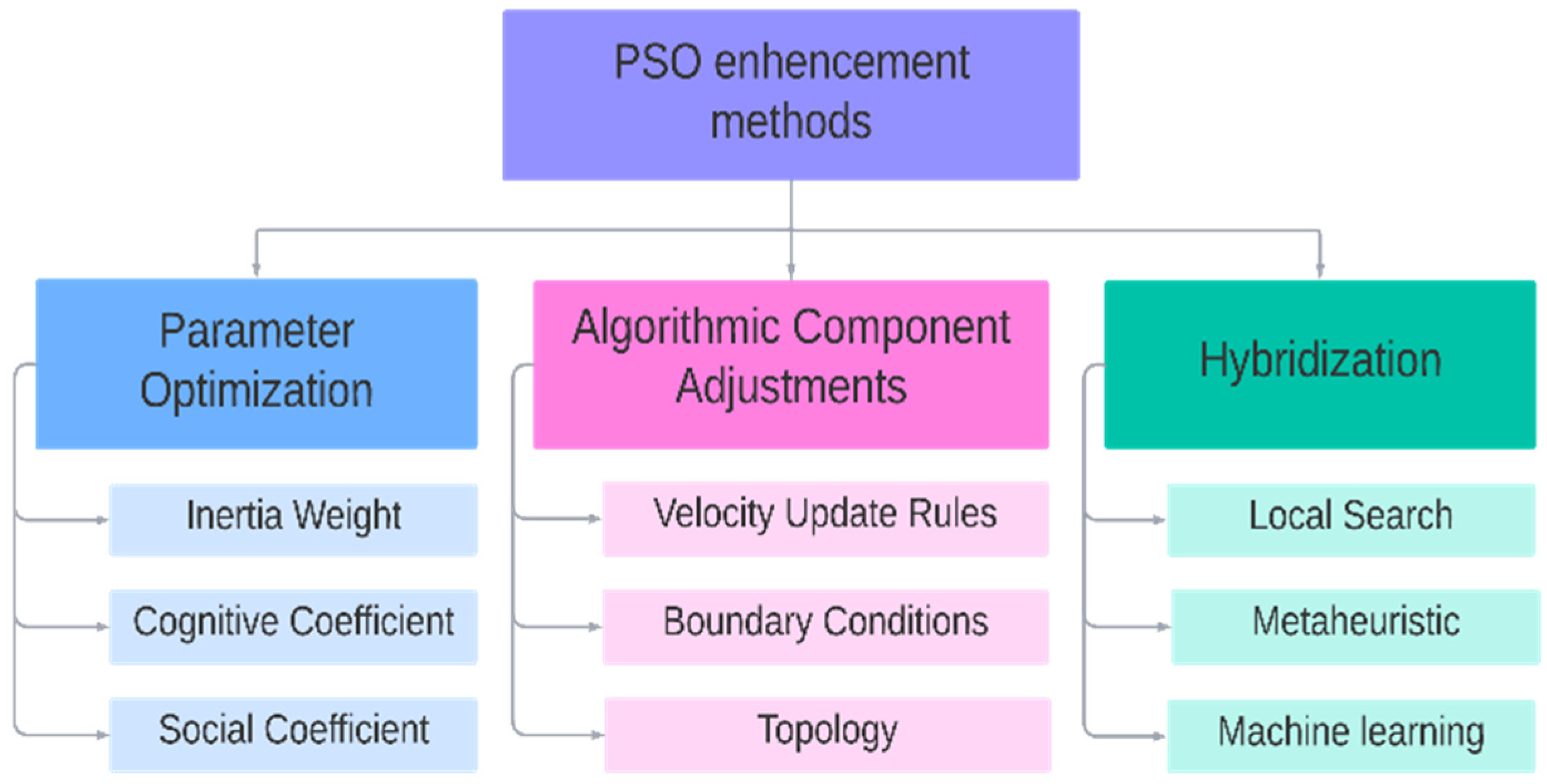
Several strategies have been established to improve Particle Swarm Optimization (PSO) in the past decade. Improvements in PSO have been categorized into three key methodologies, as shown in Figure 1: parameter optimization [9], algorithmic component adjustments [10], and integration with other algorithms (hybridization) [11]. Parameter optimization entails fine-tuning PSO settings, including topology, coefficients for acceleration and inertia, and population size. Adjustments to algorithmic components involve modifying velocity or position update rules, which may include creating or recalibrating existing elements. Hybridization with other techniques allows PSO to leverage complementary algorithms, enhancing its performance and problem-solving capabilities.

Firstly, parameter setting for PSO algorithm has caused significant difficulty in the area of iterative optimization techniques in recent years [12]. Recent research [13,14] has identified two primary approaches to parameter setting: parameter tuning and parameter control.

Parameter tuning entails establishing the algorithm’s parameters to specific values found via simulations [15]. This approach has also been applied in airline scheduling problems [16,17], where a Hidden Markov Model was investigated for tuning metaheuristics [18]. In contrast, parameter control refers to the process of dynamically modifying parameter values while the algorithm is running [19,20]. This method can be classified into static, adaptive, or self-adaptive approaches.

Static parameter control utilizes some pre-established rules, sometimes referred to as a time-varying rule, to modify parameter values depending on the PSO iteration number [21]. Adaptive control of parameters employs some function to establish a relationship between the feedback obtained from the current optimization process and the value of the PSO parameter [22].

In a previous work [8], a Hidden Markov Model (HMM) was used as an online classification method to estimate PSO states, which are exploration, exploitation, convergence, and jumping out [23]. The earlier approach adaptively adjusts the acceleration factors c1 and c2. In [9], an equivalent HMM-based approach was applied to adapt the population size along with the acceleration factors. Another work [24] leveraged HMM-detected PSO states to control the inertia weight also using HMM classification.

Self-adaptive parameter control embeds the parameters within each particle, enabling these parameters to vary and develop during the algorithm’s execution [25]. Notably, the use of a classification model has been explored for adapting PSO parameters, providing a probabilistic framework for dynamic adjustments, like in [26], where the authors proposed a probabilistic finite state machine design for self-parameter adaptations of each particle in PSO, enhancing its adaptability and robustness. Similarly, the authors of [23] further incorporated a self-dynamic adaptation of population size across iterations.

Additionally, PSO parameter adjustment may be performed in two contexts: homogeneous and heterogeneous swarms [27]. In a homogeneous swarm, all particles exhibit uniform behavior, but in a heterogeneous swarm, several distinct behaviors coexist concurrently [28]. Recent studies have introduced cooperative multi-swarm strategies and adaptive cooperation using a Markov Model, enhancing the performance and robustness of PSO in various applications [29,30].

Furthermore, the authors of [20,31] presented an in-depth investigation of the latest advances in PSO, exploring different parameter control methodologies and real-world applications. The research results jointly give important insights into the techniques and the resulting impacts on the PSO algorithm.

Other recent advancements in Particle Swarm Optimization (PSO) have focused on enhancing key algorithmic components, including velocity update rules, boundary conditions, and topology structures. These components are crucial for the overall performance, stability, and convergence of PSO algorithms. The velocity update calculus in Particle Swarm Optimization (PSO) is essential for managing particle movement and ensuring successful convergence. The authors of [32] presented adaptive velocity update techniques that dynamically alter parameters depending on the optimization process. Their analysis gives insights into how these updates boost PSO’s convergence and stability. Meanwhile, managing boundary conditions efficiently is essential for maintaining the search space’s integrity and preventing particles from running away. The authors of [33] addressed unique boundary management approaches that retain particle diversity while preserving search space boundaries. Their thorough review underlines recent measures and their influence on PSO performance.

Additionally, the topology of PSO specifies the structure of communication links within particles, significantly affecting the algorithm’s efficiency. The authors of [14] examined different topology patterns and their effects on PSO achievement. Their work offers suggestions for choosing suitable structures based on specific optimization problems. Also, the authors of [29,30] examined cooperative plans through PSO topologies, emphasizing the advantages of multi-swarm cooperation and adaptive communication frameworks. These studies indicate how cooperative strategies may boost PSO performance by enhancing exploration and exploitation balance and strengthening the robustness of the optimization process.

Hybridization in PSO leverages multiple strategies to increase the algorithm’s effectiveness. The authors of [34] reported that hybrid approaches have shown success in resolving complex optimization problems and therefore validated the usefulness of combining PSO with local search methods, meta-heuristics, and machine learning. One hybrid strategy involves adding local search methods to refine solutions near potential regions determined by PSO, which aids in attaining quicker convergence and more accurate solutions. For example, the authors of [35] combined dynamic multi-PSO with gravitational search algorithms to solve complex optimization problems. Another hybrid approach involves combining PSO with other metaheuristics like simulated annealing or a genetic algorithm, balancing their strengths to avoid local optima and the premature convergence phenomenon. The authors of [36] demonstrated a hybrid PSO–firefly algorithm to enhance cloud performances. The authors of [37] proved that integrating the global search capacity of genetic algorithms with the convergence speed of PSO will result in a significant improvement compared to other methods.

Integrating machine learning with PSO enables adaptive parameter control and dynamic modification of the algorithm’s behavior. Techniques like supervised learning [38] and deep learning [39] have been utilized to inform and optimize PSO’s parameter adjustments effectively. For instance, the authors of [40] used a multilayer PSO with ANN, adapting network topology and synaptic weights. This adaptive approach allowed for the dynamic control of parameters, boosting optimization efficiency and accuracy. The authors of [41] proposed one reinforcement learning-based parameter adaptation approach for PSO, showcasing its effective and adaptive capabilities. This approach was further validated in a recent study [42], emphasizing the usefulness of reinforcement learning hybridized with PSO for suitable adaptation. Such models can predict optimal settings, assess the optimization state, and guide the search process, significantly enhancing PSO’s efficiency [43,44]. They also handle complex optimization challenges, solidifying PSO’s role as an effective and versatile hybrid optimization method.

3. Deep Q-Network-Based Adaptive PSO

This section describes the background knowledge, some essential concepts of the literature, and our previous algorithm, HMM-APSO [8], which provided the foundation for presenting our parameter adaptation control method using a Q-network. The suggested technique is about dynamically balancing the states of PSO to identify optimal parameter values which assure success in different optimization settings. Using a Hidden Markov Model (HMM) helps identify these appropriate states via analyzing the evolution and transitions all over the PSO iterations. Once the most suitable state is determined, establishing a Deep Q-Network (DQN) permits the selection of the optimal action, indicating the best suited parameter values in that state. This combination provides adaptive and strategic adjustments to PSO parameters, boosting performance by dynamically modifying the algorithm. This dynamic adaptation helps strike a balance between PSO states, leading to higher convergence and improvements in accuracy.

3.1. Theoretical Framework

Regarding the new approach proposed this work, we utilize the classical version of Particle Swarm Optimization (PSO) given in [45], which features a global topology where each particle is connected to every other particle and influenced by the global best (gBest) particle. Each particle i is described by two vectors: velocity vector $v_i$ and position vector $x_i$. The following equations define how those vectors are updated at each iteration $t$:

$$v_i(t+1)=w{v}_i\left(t\right)+c_1{r}_1({pBest}_i-x_i(t\left)\right)+c_2{r}_2(gBest-x_i(t\left)\right)$$

(1)

$$x_i(t+1)=x_i\left(t\right)+v_i(t+1)$$

(2)

We assume that there are N particles of the swarm in S space. Here, i indicates the particle’s index, and t is the iteration’s index; $r_1$ and $r_2$ are defined in the interval [0,1], representing two independently and uniformly distributed random variables. The inertia weight w is generally adjusted to decrease linearly from 1 to 0 throughout the execution. The constants $c_1$ and $c_1$ are named acceleration factors. ${pBest}_i$ indicates the personal best position of particle $i$. $gBest$ refers to the global best position.

In Figure 2, the diagram shows the iteration steps of PSO. The stopping criteria commonly have a maximum number of loops or some convergence criteria.

3.2. Markov Chain on PSO

PSO can be analyzed by examining its stochastic behavior as a multi-stochastic process. As identified by previous researchers, notable work on PSO is based on empirical studies using simulations, and less work has been conducted to analyze PSO theoretically. In [46], a few theoretical propositions were utilized to explore the stochastic process of PSO.

According to [47], the PSO state takes into account as much detail as possible in the process. Previous researchers [46] have proven that the PSO state is memory-less. The state was defined by

$$ST\left(t\right)=(X\left(t\right),\mathrm{p}\mathrm{b}\mathrm{e}\mathrm{s}\mathrm{t}\left(t\right),\mathrm{V}\left(t\right),gbest\left(t\right))$$

(3)

W is called a state at time t. It proved the stationarity of the Markov chain on the PSO. We assume that the information contained in W(t) is enough for future moves, and it depends only on the actual iteration state and not the past iteration state. The effect of the current state on the future states is not dependent on its past states. Thus, PSO’s behavior only depends on the actual state, not on the succession of the past, which rides on previous achievements.

To evaluate the success of the state, ST, in PSO, an index is defined to reflect the current accomplishment based on particle positions and probability concepts due to their stochastic movements. These states are categorized into classes identified as levels. The levels follow a stochastic process described as

$$\left\{L\left(ST\left(t\right)\right),t=\mathrm{1,2}\dots \right\}$$

(4)

Forming a Markov chain [48,49,50] on PSO levels, this approach, detailed in [46], ensures the achievement is position-dependent, aligning with the probabilistic nature of particle movements.

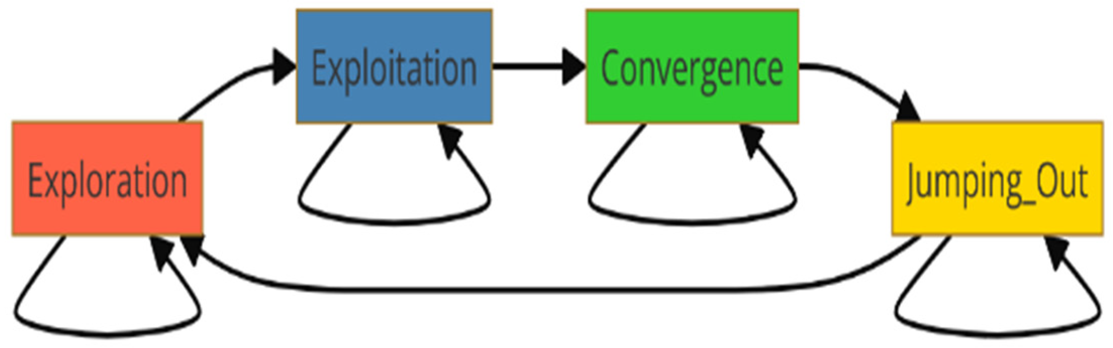
We define, as shown in [51], four evolutionary levels considered as a global state of the PSO swarm, namely the following:

L = {exploration, exploitation, convergence, jumping out}.

The Markov chain represents the PSO states in Figure 3. The arrows show the possible transitions between states.

Although the exploration state describes the process of looking at a large area in solution space to avoid local optima, in the exploitation state, the swarm adjusts the solution at the best-known locations to serve the purpose of accuracy. The convergence state involves stable particles, and it is focused on the optimal solution so that the best results may be reached. The jumping-out state adds randomness to escape local optima and continue seeking the global optimum, maintaining variety and avoiding premature convergence. One must balance these states of PSO, giving the appropriate parameter setting for it to be successful when used in optimization situations.

3.3. Partially Observed Markov Decision Process in PSO

Based on the previous paragraph, we define a POMDP [52] on the PSO to build a model of control and adaptation of PSO parameters according to the swarm state. We can characterize a POMDP over PSO since there are already PSO states in the swarm: L = {exploration, exploitation, convergence, jumping out}. The state of each particle is not directly observable. Still, it is inferred through an evolutionary factor $f$ that reflects the relative positions of particles and is defined by the average distance of each particle to all others, as described in [51]. The actions are variations in the PSO parameters, and the reward is the measured enhancement of the best solution. This approach gives a perfect way for PSO to dynamically control and optimize its parameters based on the observed swarm behavior.

Formally, the POMDP is defined as a tuple $\left(S,A,T,Z,R,b_0\right)$ as follows:

• States (S)

$$S=\left\{s\right|s\in L\}$$

(5)

• Observations (O)

$$O=\left\{o\right|o=f\left(Gbest\right)\}$$

(6)

$f\left(Gpest\right)$ is the mean distance of Gbest to all other particles:

$$f\left(Gpest\right)=\left|{\displaystyle \frac{d_{gbest}-d_{min}}{d_{max}-d_{min}}}\right|\in \left[0,1\right]$$

(7)

where $d_i$ is the distance between a particle $i$ and the other particles.

• Actions $\left(A\right)$:

$$A=\left\{a\right|aisacombinationofPSOparameterssettings\}$$

We define four parameters setting combinations ${\left\{A\right\}}_1^4$.

Actions include setting values for inertia weight, cognitive coefficient, social coefficient, and randomness.

• Transition Model (T):

$$T(s,a,s\prime )=P\left(s^{\prime }\right|s,a)$$

(8)

$T$ is the probability of transitioning from state $s$ to state $s’$ given an action $a$.

• Observation Model (Z):

$$Z(s\prime ,a,o)=P\left(o\right|s\prime ,a)$$

(9)

Z is the observation probability of $o$ given the next state $s\prime$ and the action $a$.

• Reward Function (R):

$$R(s,a)$$

(10)

This is the reward received after taking action $a$ in a state $s$ and the measurement enhancement of the best solution.

• Initial Belief State $b_0$: This is the initial probability distribution over states. It will be given as an exploration state with a probability equal to 1 and 0 for other states; this means that we assume an exploration state at iteration one.
• The objective is to select the actions a ∈ A that maximize the expected cumulative reward over time, accounting for the partially observable nature of the states through the observed parameter f.

Then, the policy π maps the history of observations and actions to actions such that the expected sum of rewards is maximized.

To solve this model, we conduct an approach integrating the Hidden Markov Model and Q-network [53]. It is an advantageous solution strategy due to the complementary strengths of these methods.

Using this approach, we can handle partial observability efficiently by using HMMs to maintain and update the belief state of the swarm. A belief state is a probability distribution over possible states that enables the swarm to make effective inferences about the state of its environment, even when the true state is not directly observable. It combines the powerful deep-learning approximation algorithms of complex functions for high-dimensional state spaces into the Q-network [53] used for action selection. This way, the agent can learn an optimal policy that maximizes the long-term reward while solving this partial observability problem. The state estimate generated by our proposed solution is effectively aggregated by HMMs, leading to scalable Q-networks that can be efficiently used for policy learning in POMDPs.

The following paragraphs will detail the HMM and Q-network models.

3.4. HMM Belief State Classification

The Hidden Markov Model (HMM) is used for PSO state classification due to its advantage in sequence analysis, notably in voice recognition and classification domains. HMMs have proven effectiveness for sequence analysis [54], especially in representing systems with hidden states and time-dependent interactions. This results from their capacity to manage sequential data with inherent stochastic processes. Algorithms including Baum–Welch and Viterbi allow HMMs to continually estimate model parameters while identifying the most probable sequence of hidden states, thereby enhancing accurate classification and prediction in intricate temporal patterns.

We set the HMM with a triple $(\mathsf{\Pi },\mathrm{A},\mathrm{B})$, and $(\mathsf{\Omega },F,P)$ is a probability space where the whole processes are defined:

• $\mathsf{\Pi }=\left({\mathsf{\pi }}_{\mathrm{i}}\right)$, the vector representing initial state probabilities. Π = [1 0 0 0]: Initial state probability specifying a first deterministic initialization in the exploration state.
• $\mathrm{A}$ = $\left({\mathrm{a}}_{\mathrm{i}\mathrm{j}}\right)$, the transition matrix between states, $\mathrm{P}(X_t=i|X_{t-1}=j)$, $i,j\in [1,N]$. We supposed a 1/2 value of transition probabilities for all possible transitions in Figure 3.
• $B=\left(b_{jk}\right)$, the emission matrix named likewise a confusion matrix, $P(Y_t=k|X_t=j)$, $j\in \left[0,\mathrm{N}\right],k\in [0,M]$.

The evolutionary factor f, representing particle distribution in a search, is used as an observation source in the Hidden Markov Model. Since f is continuous within $[0,1]$, it is discretized into seven subintervals [23]:

$$\left[\mathrm{0,0.2}\right),\left[\mathrm{0.2,0.3}\right),\left[\mathrm{0.3,0.4}\right),\left[\mathrm{0.4,0.6}\right),\left[\mathrm{0.6,0.7}\right),\left[\mathrm{0.7,0.8}\right),\left[\mathrm{0.8,1}\right]$$

(11)

Each value of f is assigned to an interval, resulting in a discrete state based on the interval number. Then, matrix B has dimensions of $4\times 7$.

Probabilities are deduced from an earlier work [23] as follows:

$$B=\left[\begin{array}{ccccccc}0& 0& 0& 0.5& 0.25& 0.25& 0\\ 0& 0.25& 0.25& 0.5& 0& 0& 0\\ {\displaystyle \frac{2}{3}}& {\displaystyle \frac{1}{3}}& 0& 0& 0& 0& 0\\ 0& 0& 0& 0& 0& {\displaystyle \frac{1}{3}}& {\displaystyle \frac{2}{3}}\end{array}\right]$$

(12)

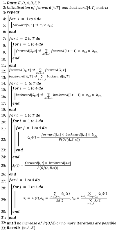
where once the parameters of the HMM are initialized, the Algorithm 1 Baum–Welch algorithm [55] is employed to compute and update the emission and transition probabilities iteratively. This process enhances the accuracy and adaptability of the HMM during the classification stage.

Algorithm 1: Baum–Welch Algorithm [55]

Subsequently, at each iteration, the Viterbi algorithm [56] is utilized to estimate the belief state of the swarm. Algorithm 2 shows the pseudo-code which describes the state sequence $\mathrm{Q}$ (where $\mathrm{Q}={\mathrm{q}}_1{\mathrm{q}}_2\dots .{\mathrm{q}}_{\mathrm{T}}$) assuming a succession of observations O ($\mathrm{O}={\mathrm{o}}_1{\mathrm{o}}_2\dots .{\mathrm{o}}_{\mathrm{T}})$. Transitions between the four states are adjusted based on the classifications provided by the HMM.

Algorithm 2: Viterbi algorithm [56]

Additionally, for each state of the swarm as determined by the HMM classification, the subsequent actions are determined by the Q-network, as detailed in the following paragraph.

3.5. Deep Q-Network-Based Parameter Setting Actions

After determining the belief state of the PSO, the Q-network is used to determine the suitable action that corresponds to the parametric adjustment control of the PSO. The Q-network, specifically the Deep Q-Network (DQN), is a kind of neural network that will be used to approximate the Q-value function in reinforcement learning, giving the optimal action selection strategy.

A formal description of the Q-network’s architecture is provided in Figure 3:

• The input layer of four possible values and four dimensions: state 1 $[1,0,0,0]$, state 2 $[0,1,0,0]$, state 3 $[0,0,1,0]$, and state 4 $[0,0,0,1]$.
  So, we have four neurons, each representing one element of the one-hot encoded state vector. It will receive the state representation of the belief state in the POMDP calculated previously by the HMM classification. Each neuron in this layer corresponds to one element of the state.
• Hidden layers include a fully connected layer with h1 = 32 neurons and ReLU activation.
• The output layer of dimension 4 that corresponds to the number of possible actions.

Q-values that represent the expected cumulative reward for each action in the provided state are determined as follows:

$$Q\left(s,a\right)=fitness\left({gBest}_{i-1}\right)-fitness\left({gBest}_i\right)$$

(13)

Fitness is the fitness function used in PSO, and $i$ is the iteration number; we are supposed to have a minimization problem.

The pseudo-code of the Algorithm 3 DQN algorithm is as follows:

Algorithm 3: DQN algorithm [57]

Regarding the action set, each of the four actions defines the parameter setting of acceleration coefficients and inertia weight. The parameter adaptation is carried out according to four actions:

• Action 1:

  -

  Random values of inertia weight between $w_{min}$ and $w_{max}$:

  $$w_i=w_{min}+\left(w_{max}-w_{min}\right)\ast rand\left(\right)$$

  (14)

  $rand\left(\right)$: the function that generates random values in [0,1].

  -

  Increase $c_1$ and decrease $c_2$.

• Action 2:

  -

  The inertia weight is calculated according to its distance from other particles:

  $$w\left(\mathrm{f}\right)={\displaystyle \frac{1}{1+1.5{\mathrm{e}}^{-2.6\mathrm{f}}}}\in [0.4,0.9]\forall \mathrm{l}\in [0,1]$$

  (15)

  -

  Increase $c_1$ and slightly decrease $c_2$.

• Action 3:

  -

  The maximum value of $w=w_{max}$.

  -

  Slightly increase $c_1$ and decrease $c_2$.

• Action 4:

  -

  The minimum value of the inertia weight: $w_i=w_{min}$.

  -

  Decrease $c_1$ and increase $c_2$.

These parameter variation actions are deduced from the best-known literature on PSO parameters’ online control, such as [24,51].

The complete applied framework for adapting the parameters in PSO is described in the next paragraph.

3.6. The PSO-Based DQN Algorithm

The parameter adaptation of PSO will be carried out according to the POMDP presented earlier. The POMDP framework enables the modeling of uncertain environments, providing a robust mechanism for dynamically adapting the parameters of PSO based on the actual state and observations. In this approach, a Hidden Markov Model (HMM) will be used to identify hidden states that correspond to various ways of adapting the optimization process, including exploration, exploitation, jumping out, and convergence. By recognizing these hidden states, the HMM can adequately track the optimization dynamics and provide information for the following actions. The DQN, with its advanced deep learning capabilities, will subsequently choose the most appropriate strategy for selecting actions in each recognized state. The following Algorithm 4 illustrates the approach steps.

Algorithm 4: DQNPSO

The PSO method is designed to optimize its parameters by maintaining a balance between exploring new solutions and exploiting established, highly effective ones. It is also successful at escaping local optima and rapidly converging to optimum solutions, enhancing overall performance. An experimental study was conducted, and it is described in the following section to display the effectiveness of the newly adopted method.

4. Experimental Study

We empirically evaluated the provided approach for adapting PSO parameters based on HMM and DQN. We simulated several benchmark functions, including unimodal and multimodal categories. Subsequently, the findings are compared with those obtained from other modern PSO variations to evaluate our method’s efficiency.

4.1. Parameters Configuration

Several interconnected variants of the PSO algorithm from the literature were chosen for comparison during testing (

Table 1. The selected PSO variants from the literature.

Algorithm	Name	Specific Settings	Reference
APSO	Adaptive PSO	$c_1=c_2=2,\omega =0.9$	[51]
LinWPSO	Linear decreasing weights PSO	${\omega }_{min}=0.0001,{\omega }_{max}=0.1$	[58]
AsyLnCPSO	Asynchronous PSO	${c_1}_{min}={c_2}_{min}=0.01$,${c_1}_{max}={c_2}_{max}=2$	[59]
RandWPSO	Random inertia weight PSO	$c_1=c_2=2,{\omega }_{min}=0.01,{\omega }_{max}=0.9$	[60]
YSPSO	PSO with compressibility factor	$c_1=c_2=2,\omega =0.9$	[61]
SecVibratPSO	Order oscillating PSO	$c_1=c_2=2,\omega =0.9$	[62]
CLSPSO	Cooperative line search PSO	$c_1=c_2=2,\omega =0.9$	[63]

).

The suggested DQNPSO approach was simulated and validated on many benchmark functions (see

Table 2. Standard test functions.

Function	Name	Category
${\mathbf{f}}_1={\sum }_{\mathbf{i}=1}^{\mathbf{D}}\left[{{(10}^6)}^{{\displaystyle \raisebox{1ex}{$\mathit{i}-1$}\!\left/ \!\raisebox{-1ex}{$\mathit{D}-1$}\right.}}{\mathit{x}}_{\mathit{i}}^2\right]$	Elliptic	Unimodal
${\mathbf{f}}_2={\sum }_{\mathbf{i}=1}^{\mathbf{D}}\left(\right|{\mathbf{x}}_{\mathbf{i}}+0.5|{)}^2$	Step	Unimodal
${\mathbf{f}}_3={\sum }_{\mathbf{i}=1}^{\mathbf{D}}{{\mathbf{x}}_{\mathbf{i}}}^2$	Sphere	Unimodal
${\mathbf{f}}_4=10^6{{\mathbf{x}}_1}^2+{\sum }_{\mathbf{i}=2}^{\mathbf{D}}{{\mathbf{x}}_{\mathbf{i}}}^2$	Tablet	Unimodal
${\mathbf{f}}_5={\sum }_{\mathbf{i}=1}^{\mathbf{D}}({\sum }_{\mathbf{i}=1}^{\mathbf{D}}{\mathbf{x}}_{\mathbf{i}}{)}^2$	Quadric	Unimodal
${\mathbf{f}}_6={\sum }_{\mathbf{i}=1}^{\mathbf{D}}[{{\mathbf{x}}_{\mathbf{i}}}^2-10\mathbf{c}\mathbf{o}\mathbf{s}(2\mathsf{\pi }{\mathbf{x}}_{\mathbf{i}})+10]$	Rastrigrin	Multimodal
${\mathbf{f}}_7=-20\mathbf{e}\mathbf{x}\mathbf{p}(-0.2\sqrt{{\displaystyle \frac{1}{\mathbf{D}}}}{{\mathbf{x}}_{\mathbf{i}}}^2)$	Ackley	Multimodal
${\mathbf{f}}_8={\displaystyle \frac{1}{4000}}{\sum }_{\mathbf{i}=1}^{\mathbf{D}}{{\mathbf{x}}_{\mathbf{i}}}^2-\mathsf{\Pi }\mathbf{c}\mathbf{o}\mathbf{s}({\mathbf{x}}_{\mathbf{i}}/\sqrt{\mathbf{i}})+1$	Griewang	Multimodal
${\mathbf{f}}_9={\sum }_{\mathbf{i}=1}^{\mathbf{D}}{\mathbf{x}}_{\mathbf{i}}\mathbf{s}\mathbf{i}\mathbf{n}\left(\sqrt{{\mathbf{x}}_{\mathbf{i}}}\right)$	Schewefel	Multimodal
${\mathbf{f}}_{10}=-{\displaystyle \frac{1+\mathbf{c}\mathbf{o}\mathbf{s}(12\sqrt{{{\mathbf{x}}_1}^2}+{{\mathbf{x}}_2}^2)}{1/2\left({{{{\mathbf{x}}_1}^2+\mathbf{x}}_2}^2\right)+2}}$	Drop wave	Multimodal

).

The empirical study was carried out by iteratively conducting simulations ten times, with identical beginning parameter values. The population size was set to 30, with each particle having a dimension of 30. In each execution, a total of 1000 generations were executed. The inertia weight was set by default to specific settings given in Table 1. The parameters $c_1$ and $c_2$ were initialized with the value 2. The learning rate for the DQN was fixed at a value of 0.001, and the number of steps was 10. The tests were executed on a system with a configuration of an Intel i7 10th-generation processor and 16 GB of RAM. We focus on two performance metrics: solution accuracy and convergence speed.

4.2. Solution Accuracy

In order to assess the efficacy of our DQNPSO approach, we performed a comparison study by testing it against several PSO variations utilizing benchmark test functions. Each benchmark function was performed over all PSO variations, and the mean and best values were obtained to evaluate the solution accuracy when measured against other PSO variants published in the literature. The findings of this comparison are shown in

Table 3. Comparative analysis of PSO variant results.

Functions		DQNPSO	PSO	APSO	YSPSO	LinWPSO	CLSPSO	AsyLnCPSO	RandWPSO	SecVibratPSO
${\mathit{f}}_1$	Best	0.010212	241×106	29 × 106	367 × 106	372 × 106	7734 × 106	222 × 106	4451 × 106	911 × 106
	Mean	6.7226	7646×106	134 × 106	1074 × 106	624 × 107	292 × 108	1002 × 106	1262 × 106	22,265 × 106
${\mathit{f}}_2$	Best	0	9.13×10−6	0	0	0	0	0	0.00001166	16,867
	Mean	0	0.21843	0	0	0	11,393	1.41 × 10−25	23,771	92,849
${\mathit{f}}_3$	Best	7.104 × 10−6	292,268	48,545	73,068	159,127	716,543	165,327	272,797	46,138
	Mean	0.00175	463,932	24,973	14,448	31,6226	2,259,075	408,782	607,237	647,525
${\mathit{f}}_4$	Best	1.67 × 10−5	985,342	11,408	220,672	34,463	2,021,904	240,971	1,186,314	3888
	Mean	0.00348	164,255	42,255	418,765	1,054,338	4,028,212	439,076	2,111,731	1,951,189
${\mathit{f}}_5$	Best	0.38443	2.44×1011	871 × 106	170 × 107	3484 × 107	2.050×1012	369 × 108	6.586 × 1011	1325 × 107
	Mean	624.22	1.61×1012	8934×106	6950 × 107	9.927×1011	7.07×1012	1856 × 107	3.105 × 1012	6.228 × 1012
${\mathit{f}}_6$	Best	0.000115	2,189,475	373,897	1,099,642	170,471	3,712,168	1,977,706	2,043,068	2,095,081
	Mean	3.6364	3,074,856	573,572	1,821,846	2,583,946	5,351,072	2,905,228	3,133,353	3,280,662
${\mathit{f}}_7$	Best	0.000725	47,818	14,562	3659	44,627	73,411	45,955	48,573	18,349
	Mean	0.020312	56,504	22,541	44,661	54,669	94,979	5951	58,876	51,858
${\mathit{f}}_8$	Best	5.46 × 10−8	15,527	59,507	71,176	13,023	38,083	68,348	15,657	39,343
	Mean	0.01632	38,999	26,352	16,698	32,301	75,682	19,472	53,535	46,518
${\mathit{f}}_9$	Best	0.012693	572,305	33,239	155,126	325,646	1,583,686	186,099	68,254	108,678
	Mean	3.6911	995,474	563,267	247,067	663,407	4,052,457	587,928	1,769,817	2,338,293
${\mathit{f}}_{10}$	Best	−1	−99,999	−1	−1	−1	−1	−1	−99,297	−9943
	Mean	−1	−9599	−9856	−98,972	−96,298	−94,403	−99,383	−94,333	−82,273

.

We can see in Table 3 that DQNPSO enhances PSO when compared to the selected PSO variants from published research. There is a considerable improvement across DQNPSO compared to the other techniques. Our suggested approach delivers much superior results. DQNPSO has developed considerably higher solution accuracy efficiency for unimodal and multimodal functions.

4.3. Process Time

We analyzed the process time of the DQNPSO approach against other PSO variants based on the CPU execution time for all benchmark functions. Since the execution is performed solely on the CPU without any parallelism or GPU implementation, our focus is exclusively on the CPU time.

The execution durations of several PSO variants are illustrated in Figure 4. It emphasizes that DQNPSO has execution durations that are substantially longer and more variable than other PSO variants. This is a result of the use of a Deep Q-Network (DQN), which incorporates complex neural network computations. The execution durations of the other PSO variants, including APSO, PSO, LinWPSO, and others, are consistently lower and more predictable, suggesting more efficient and reliable performance. This implies that DQNPSO operates at the expense of computational efficacy. However, the high accuracy performance demonstrated in the previous paragraph can largely compensate for this time consumption. In addition, this issue of CPU time consumption can be addressed, and we can implement GPU execution and incorporate parallelism capabilities into our algorithm. This approach is supported by studies such as [64].

4.4. Convergence Speed

We conducted a comparison regarding the convergence speed for the ten benchmark functions.

The charts used for the comparative analysis of the convergence speed are presented in Figure 5. The red line of the DQNPSO executions’ cross-iterations is below all other chart lines. Consequently, DQNPSO delivers a speedier convergence than the previously employed PSO variations in the literature.

4.5. Statistical Test Evaluation

To further compare DQNPSO with other selected PSO algorithms, we employed parametric two-sided testing, specifically the t-test, at a 0.05 significant level. Using this method makes it easier to assess whether the observed performance differences are due to chance and whether they are statistically significant [65]. Using the 0.05 criterion enabled us to definitely determine whether DQNPSO exhibits real gains over other PSO algorithms or if the observed changes lack a significant effect. The t-test findings define the outcomes as significant (p-value < 0.05), marginally significant (0.05 ≤ p-value < 0.1), or not significant (p-value ≥ 0.1), permitting a straightforward evaluation of comparative performance and providing an evidence-based foundation for analysis.

The statistical comparison (see

Table 4. Statistical t-test comparison of DQNPSO with other PSO algorithms.

	PSO	APSO	LinWPSO	AsyLnCPSO	RandWPSO	YSPSO	SecVibratPSO	CLSPSO
$f_1$	0	0	0	0	0	0	0	0
$f_2$	0.0260	0	0	0.0040	0.0797	0	0.0149	0.0710
$f_3$	0	0	0	0	0	0	0	0
$f_4$	0	0	0	0	0	0	0	0
$f_5$	0	0	0	0	0	0	0	0
$f_6$	0	0	0	0	0	0	0	0
$f_7$	0	0	0	0	0	0	0	0
$f_8$	0	0.0129	0	0	0	0	0	0
$f_9$	0	0	0	0	0	0	0	0
$f_{10}$	0	0.0822	0	0.0745	0	0.0536	0	0
+1 (Better)	10	9	10	9	9	9	10	9
0 (Same)	0	1	0	1	1	1	0	1
−1 (Worse)	0	0	0	0	0	0	0	0

) of DQN against multiple PSO algorithms indicates that DQN consistently outperforms other PSO versions, with only very few occasions when its performance equals that of the others. This is underscored by the large count of +1 (better) results across all comparisons, where DQN demonstrated superior performance in 90% to 100% of the cases. APSO, AsyLnCPSO, RandWPSO, YSPSO, and CLSPSO each presented a single result of 0 (Same), illustrating marginal differences where DQN performed similarly but not worse. Evidently, there were no examples of -1 (worse), indicating DQN’s robustness and better or equivalent performance across all tests. This analysis confirms DQNPSO’s strong potential compared to standard and modified PSO algorithms.

5. Conclusions

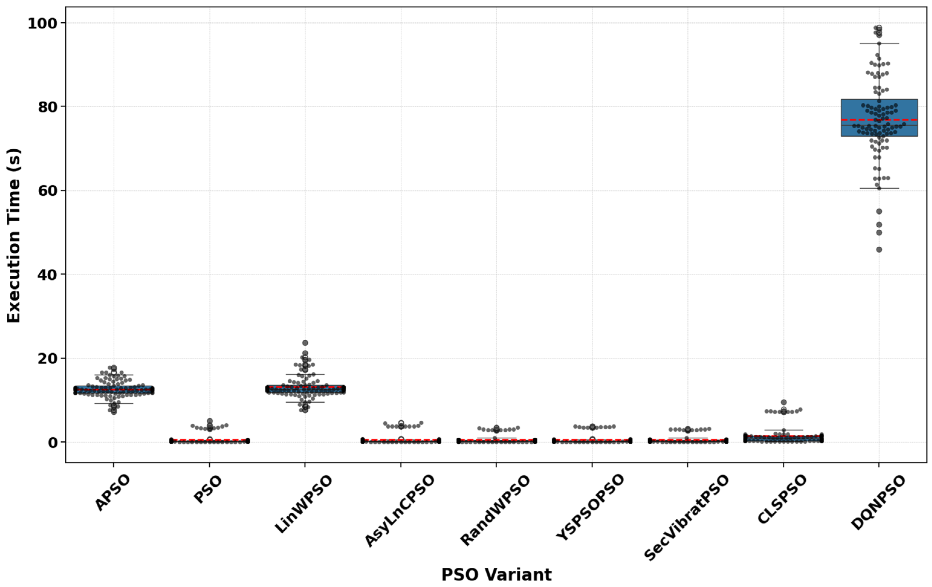
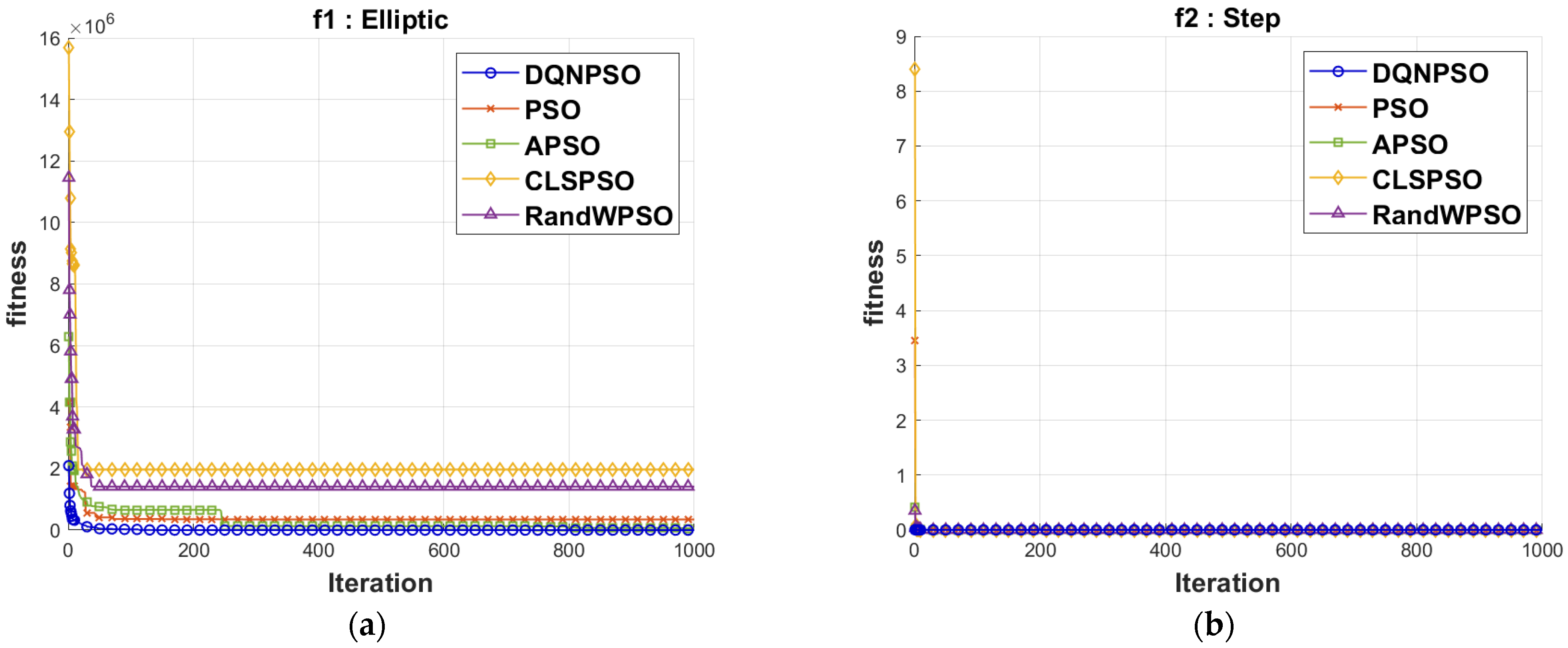
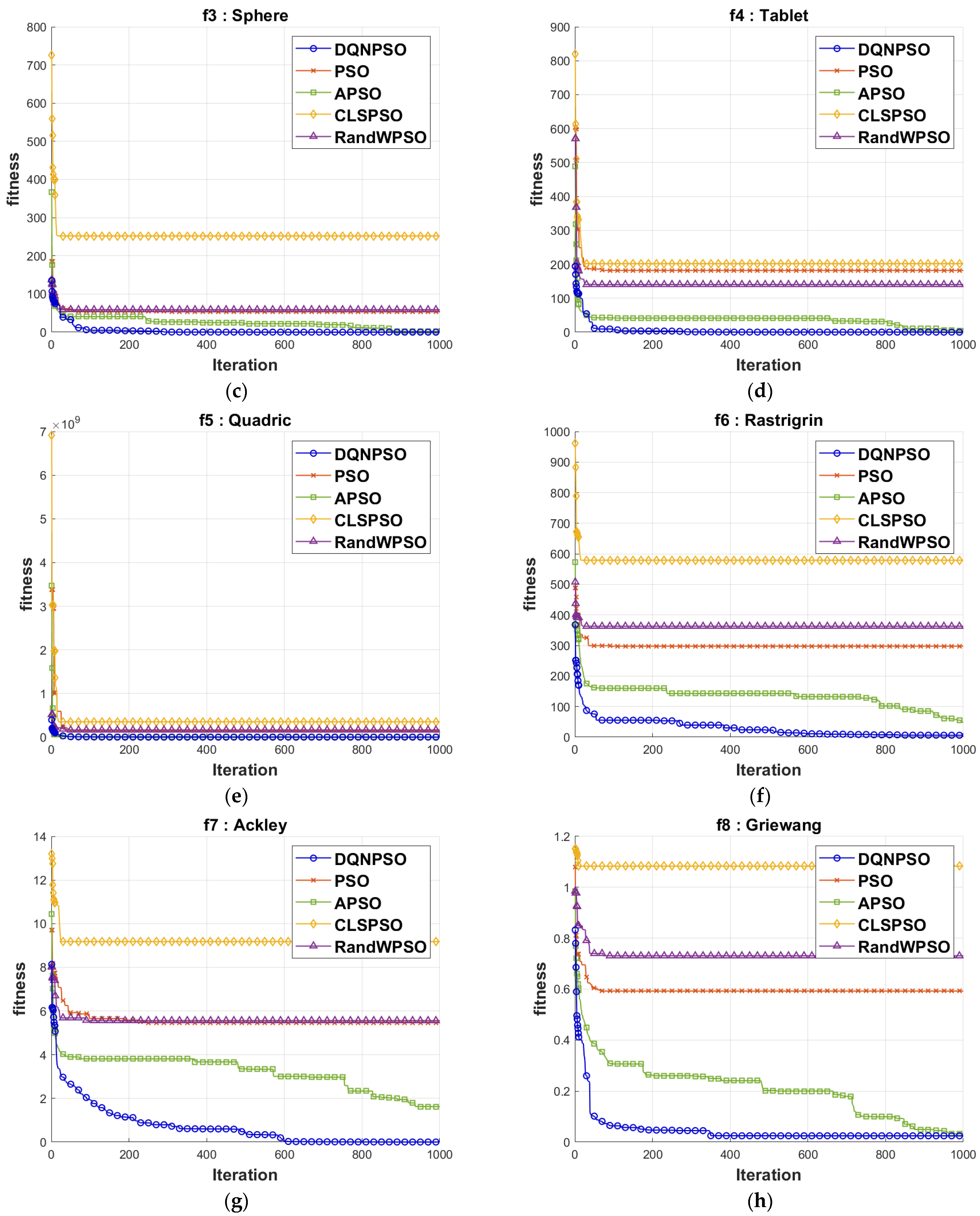
In conclusion, this research proposes significant advances in Particle Swarm Optimization (PSO) by integrating a deep machine learning approach, namely Deep Q-network, for dynamic parameter setting in a homogenous PSO framework. By solving the prevalent issues of slowing down convergence or being stuck in local optima, this suggested approach considerably boosts the entire performance of the PSO. The newly introduced DPQ-PSO framework, which combines a partly observed Markov decision process model with Hidden Markov Model classification and a Deep Q-Network, offers an adaptive method for real-time parameter adaptation. The experimental findings regarding several benchmark unimodal and multimodal functions verify the superior performance of the DPQ-PSO algorithm, providing considerable increases in solution accuracy and convergence speed compared to current techniques. However, this approach suffers from an increased CPU time due to the computational complexity introduced by the integration of deep learning. This novel method not only increases the application capacity of PSO in handling complex optimization issues but also sets a new benchmark in improving metaheuristic algorithms using deep machine learning approaches.

Future research should focus on the augmented computational time resulting from deep learning integration by exploring model optimization strategies, such as pruning the DQN parameters, alongside parallel computing methods for improved scalability. Extending DPQPSO to heterogeneous systems could increase solution variety, while integrating other advanced reinforcement learning techniques like Proximal policy optimization could further develop parameter adaptation. Furthermore, the DPQPSO framework has substantial potential for real-world applications, improving performance in several domains, and implementing this method in complex optimization tasks, such as engineering design and scheduling, will further support its efficacy.