Article

Path Planning Method for Wire-Based Additive Manufacturing Processes

1
Department of Power Engineering Machine Building and Mechanics, National Research University Moscow Power Engineering Institute, 14 Krasnokazarmennaya Street, 111250 Moscow, Russia
2
FSUE “RFNC—VNIITF Named After Academ. E.I. Zababakhin”, 111250 Moscow, Russia
*
Author to whom correspondence should be addressed.
Modelling 2024, 5(4), 2040-2050; https://doi.org/10.3390/modelling5040105
Submission received: 28 October 2024 / Revised: 10 December 2024 / Accepted: 12 December 2024 / Published: 14 December 2024

Abstract

:
The relevance of creating specialized computer programs that convert a virtual 3D model of an object into machine code (G-code) for controlling the process of 3D printing products from wire raw materials is substantiated. It is shown that for wire-based additive technologies, a fundamentally important requirement is to ensure the continuity of the surfacing trajectory within one section. A method for determining a continuous surfacing trajectory is proposed, the implementation of which requires two stages: performing a numerical analysis of a two-dimensional region with boundary conditions describing this section; and running a heuristic algorithm for the movement of the surfacing head, in which the direction of movement is selected based on the results of the analysis. The procedure for setting boundary conditions and an algorithm for numerically solving the boundary value problem of determining the field of the “height” function for each section are described. The principles of operation of the heuristic algorithm for selecting the direction of head movement based on the calculated height field and continuous determination of the proximity of adjacent layers and section boundaries are disclosed. An analysis of the algorithm operation is carried out using a section with holes as an example, and the potential of using numerical methods to calculate the change in the temperature field during the surfacing process is shown.

1. Introduction

It is known that wire-based additive manufacturing technologies are promising methods for producing medium- and large-sized products. To implement these technologies, an electric arc [1,2], plasma jet [3], laser [4], or electron beam [5] can be used as a heating source. To create a manufacturing control program, it is necessary to slice the three-dimensional model of the product into a certain number of two-dimensional layers of fixed thickness and form an individual tool movement trajectory for each layer [6,7,8]. An extremely important task is to determine the trajectory of the surfacing tool, which includes a wire feed mechanism and a heating source. Let us agree to call this tool a surfacing head and consider existing approaches to solving the problem of choosing a surfacing trajectory within one layer.
All processes based on melting the wire fed into the welding pool are characterized by a deviation in the height of the weld bead at the beginning and end of the welding (Figure 1). This is because heat exchange in these areas is not stationary [9]; initially, the molten pool is formed on a substrate that has not yet been heated, the metal is cooled more effectively, and the bead is formed higher and less wide. At the final section, the wire is no longer fed, and the molten pool will spread over the substrate, forming, on the contrary, a lower bead [10,11].
This circumstance leads to the need to minimize the number of areas where the welding path is interrupted. The simplest continuous welding trajectories are zigzag (Figure 2a) and spiral (Figure 2b). Their construction does not require complex calculations but they have significant drawbacks [11,12,13]. With a zigzag movement of the welding head, the lateral boundaries of the layer are formed in steps, and in the areas of the trajectory reversal, overheating of the metal will be observed due to the influence of reheating zones. The spiral trajectory strategy is suitable only for constructing circular sections. It should be added that both types of trajectories cannot be continuous in principle if the section contains grooves or holes (please, see the red arrows in Figure 2a,b,d).
The contour parallel strategy (Figure 2c) can solve the reproduction of both external and internal section boundaries quality problem but only for the case when both boundaries are geometrically similar and the distance between them is constant. Thus, the authors of ref. [13] rightly noted that when implementing this method, the problem of path crossing may arise (please, see red circles in Figure 2c). In other cases, it is necessary to generate several closed contours that are not connected to each other, so it is necessary to make transitions between them, interrupting the welding line.
In the hybrid strategy (Figure 2d), it is possible to reproduce smooth section boundaries and fill them using simple algorithms, for example, by moving in a snake-like pattern (zigzag); however, in the presence of grooves and holes in the contour, this method also does not allow for the construction of completely continuous trajectories.
The best results for the methods considered in [14] were found by using the pixel strategy (Figure 2e) developed by Scotti and Ferreira [13]. The pixel strategy allows for the construction of a continuous trajectory, and as the only type of defect observed during surfacing of a hollow cylinder, the authors indicated the appearance of open voids on the outer surface.
The pixel strategy consists of layer discretization on the first stage and a metaheuristic procedure for generating the trajectory of the surfacing head on the second one. In the first stage, a distribution of dots must be generated. The second stage is based the on travelling salesman problem, and it uses a metaheuristic greedy randomized adaptive search procedure (GRASP) to connect the dots continuously without intersections. According to [15], each iteration performs two perfectly defined phases: the first phase creates viable solutions to the problem, which promotes diversity; and the second phase consists of the optimization from the created solutions. The limitations of the method include the presence of a large number of turns of the welding head at angles of 45 or 90 degrees, which causes the appearance of stepped contours and defects due to limitations in the acceleration of the servomotors.
To solve the continuous path-built problem for surfacing contours with holes and grooves, a method based on the decomposition of the section by dividing it into typical solid polyhedrons has proven itself well (Figure 2f [16]). The connections of these polygonal trajectories are shown with blue circles in Figure 2f. However, if there are curvilinear or round holes in the section, the number of typical polyhedrons will have to be increased, so the trajectory will be a broken line with an excessively large number of turns, including sharp angles.
Figure 2. Path strategies for generating continuous trajectories: (a) zigzag [13]; (b) spiral [14]; (c) contour parallel [14]; (d) hybrid [16]; (e) pixel [12,14]; (f) convex polygon decomposition [16]; (g) medial axis transformation [17]; (h) level set [18].
Modelling 05 00105 g002
It is worth noting the extremely promising methods of layer analysis. They can potentially be used to determine continuous surfacing trajectories; however, at present, they have not yet been adapted to solve this problem.
These include the median axis transformation method [17] and the level set method [18]. Both methods are successfully used to find closed contours that envelop the section but still require interruption of the wire feed process and movement of the welding head between concentric contours to fill the entire layer.
The results of this analysis show the need to improve the tool path generation methods to ensure the continuity of the surfacing process throughout the entire layer cross-section. It is necessary to consider the problem in the form of two stages: analysis of the layer cross-section and construction of the line of movement of the surfacing head.

2. Methods

2.1. Layer Cross-Section Analysis
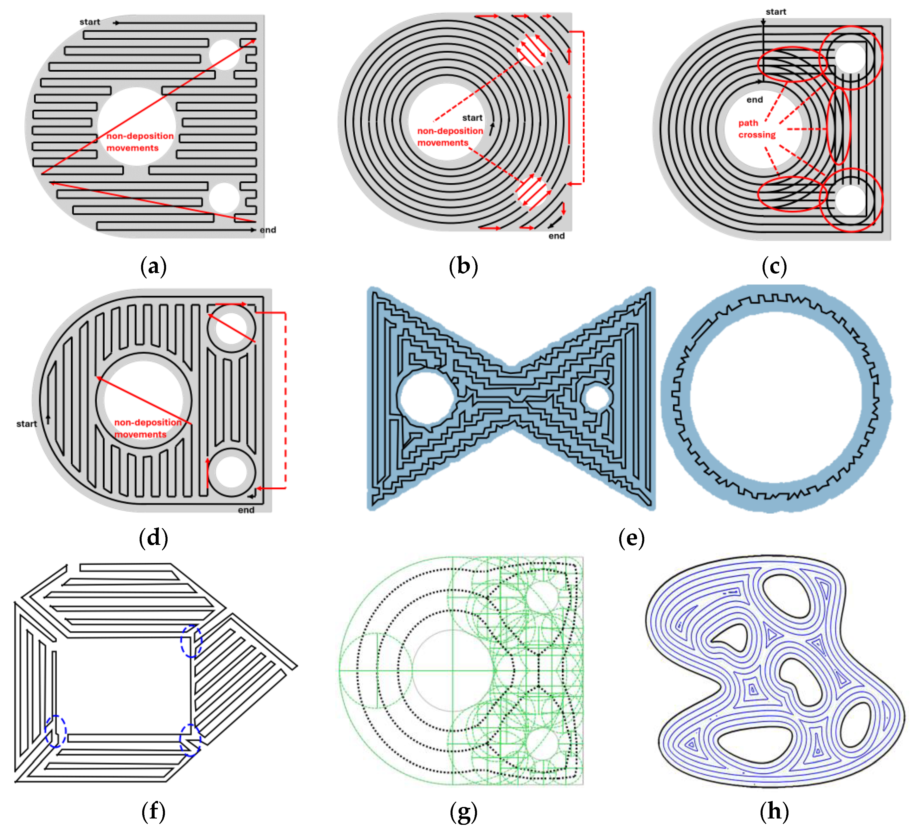
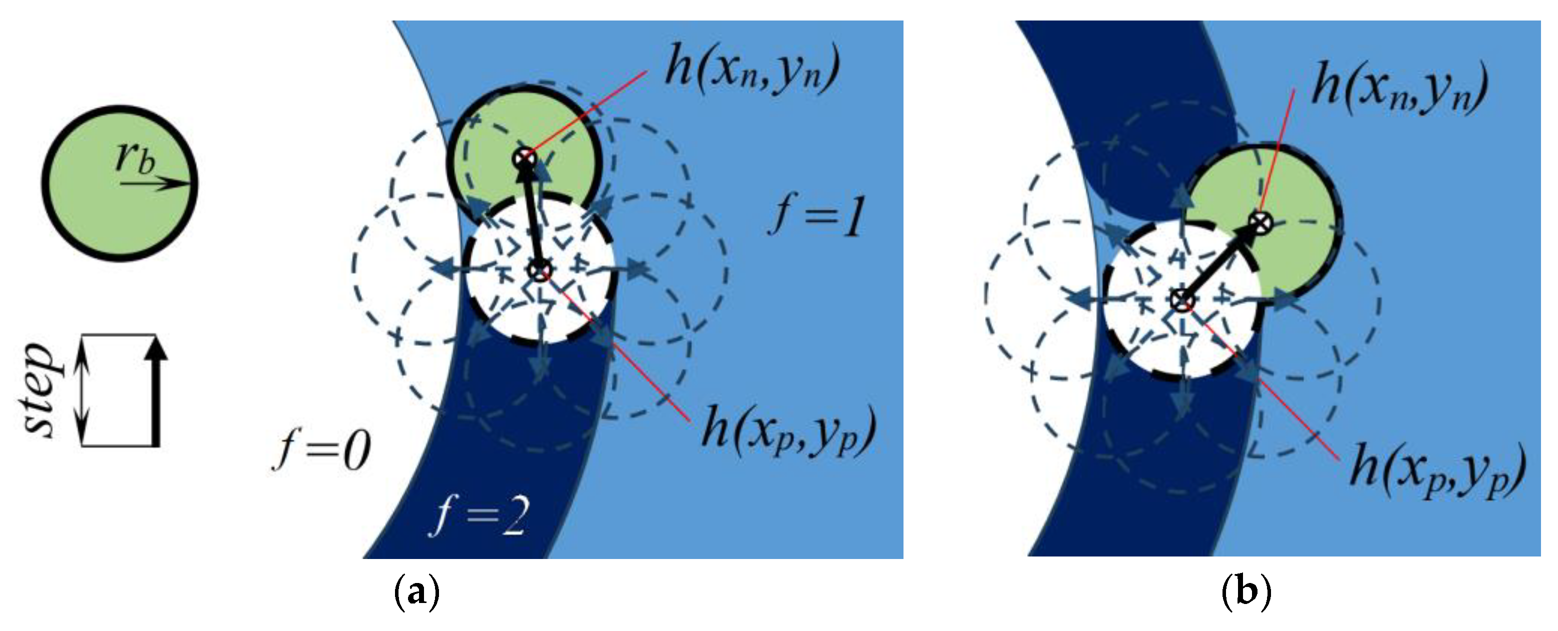
The developed analysis method is based on determining the field of a certain target function, which is a reference value for the algorithm for planning a path for moving from the center of the layer outward (or vice versa). In our case, it is convenient to interpret the function h(x,y) as a function of the imaginary layer height, just like the level set function in [18].
The analysis is reduced to solving a boundary value problem using a numerical method for solving a differential equation that describes the distribution of a scalar quantity h over a region bounded by the section under consideration and satisfying an elliptic equation:
d i v g r a d   h = 0 .
Indeed, the gradient of this function at each point will be a vector directed toward the maximum increase in height, and its absolute value will be the value of the surface “slope”. The divergence of the gradient vector field h will be a scalar value showing the curvature of the isoline at each point. There are no field sources in the problem, so the type of solution will be determined by the boundary conditions. The problem is solved by the finite difference method in a linear formulation and a grid with a uniform step in x and y is used. Then, the finite difference analogue of Equation (1) will take the following form [19]:
h i + 1 , j 2 h i , j + h i 1 , j Δ x 2 + h i , j + 1 2 h i , j + h i , j 1 Δ y 2 = 0 ,
where i and j are integer indices of control volumes of grid cells with sizes Δx and Δy (i = 0, 1, 2 … M, j = 0, 1, 2 … N).
In the problem under consideration, boundary conditions of the Dirichlet are used; that is, the function h itself is specified directly on all boundaries. The algorithm for specifying boundary conditions is a key element of the analysis stage, so it is necessary to discuss it in detail.
The reference point, at which h is taken equal to zero, is chosen at the center of mass of the section, since it is better to weld in the direction “from the inside of the section to the outside” to avoid excessive overheating of the parts. To calculate the coordinates of the center of mass in the finite-difference formulation of the problem, it is convenient to use the relations [20]:
x 0 = i = 0 M j = 0 N x i , j m i , j i = 0 M j = 0 N m i , j , y 0 = i = 0 M j = 0 N y i , j m i , j i = 0 M j = 0 N m i , j ,
where mi,j is the mass of the corresponding control volume, which vanishes outside the cross-section. After determining this point and setting the value h = 0 at it, we move on to the stage of determining the boundary conditions. To do this, using a search algorithm, the shortest distances from the region with h = 0 to all boundaries and openings (L1 and L2 in Figure 3) are determined, and in all these “empty” regions, values of h are set equal to these shortest distances.
After this, we can proceed to solving Equation (2). A typical solution in the form of isolines h is shown in Figure 3. As expected, as we approach the boundaries of the section, the shape of the isolines will approach the shape of these boundaries, and the isolines themselves will be closed, non-intersecting curves. Therefore, the field h is convenient to use as an objective function for forming the trajectory of each individual contour, which can be implemented using a tracking algorithm operating on the principle of an extremal regulator, for example, minimizing the error in deviation from the current value of h. To move from one contour to another, it is advisable to use a heuristic approach, which also requires explanation.

2.2. Path Planning

It is known that heuristic methods can provide solutions to a problem even under conditions of incompleteness or ambiguity of the stated conditions. In our case, the use of heuristics will allow us to shorten the path to solving the problem without performing a complete enumeration in the space of options [21,22].
As a rule, during surfacing, the speed of head movement, the power of the heating source, and the feed rate of the material do not change. In this case, the value of a single step of movement of the surfacing head and the transverse dimensions of the surfacing bead can be considered constant (step value on Figure 4). This is true if it is permissible to neglect deviations of the bead from the specified dimensions in height and width, which can occur due to overheating of the molten pool and repeated melting of adjacent beads. In this case, the task is reduced to determining the direction of movement of the head relative to the current position. Let us assume that for a sufficiently small step size in the shape of the layer plane, the profile of the bead will be a circle with radius rb. Let us introduce the indicator variable f = 0 for empty areas (movement into these areas is prohibited), f = 1 for layer areas in which the surfacing has not been carried out yet, and f = 2 for areas where surfacing has already been carried out (movement into these areas is prohibited too). It should be added that the starting point of the surfacing head position is defined as the area with the minimum possible value of h and f = 1. Then, the surfacing process begins, and, in the area where the surfacing head was located, the indicator variable becomes f = 2. Let us consider some arbitrary point of bead formation, shown on Figure 4.
The previous welding point has coordinates xp and yp, and the height function at this point is defined as h(xp,yp). This area is shown by the white circle. At each step, an algorithm for determining the next point of the trajectory is implemented. To determine this point, a radius vector of a fixed length (step value) is constructed from the coordinates xp, ip. The angle α of the radius vector varies from 0 to 2π and the new coordinates can be defined as follows:
x n α = x p + s t e p · cos α ,   y n α = y p + s t e p · sin α .
The algorithm uses two criteria for choosing the angle α. The first criterion is related to minimizing the deviation of h from the value at the previous point,
α = m i n h x p , y p h x n α , y n α ,
and the second criterion is to ensure the value of the indicator variable f = 1 inside the region of radius rb, with the center at the point (xn, yn) on a given fraction of the region area:
s n π · r b 2 1 s o v e r l a p .
In the last expression, sn is the part of the area with radius rb and the center at the point xn, yn (green circle on Figure 4), on which the condition f = 1 is fulfilled. The size of the area soverlap characterizes the minimum value of the mutual overlap of the beads (for intersection with areas with f = 2) or the allowance (for intersection with areas with S = 0).
To set the critical value of soverlap in case of partially occupation of green circle in Figure 4 with the areas with f = 0 and f = 2, it should be remembered that the typical machining allowance for parts built by wire-based AM methods is usually in the order of 1–3 mm [23], and the stepover distance is usually selected from the range of 0.67 … 0.738 of the width of a single bead [24].
It should also be added that the very first point of the trajectory is defined as the closest point of the layer to the center of mass that satisfies condition (6). If several points satisfy this condition, then the point with the minimum alpha is selected. Now, it is necessary to verify the performance of the described method.

3. Results

The method described above was implemented in the Microsoft Visual Studio environment in the C# language. Since the analysis of the layer cross-section is based on the numerical solution of a second-order differential equation, it is convenient to supplement the program with an algorithm for solving the heat conduction equation in a non-stationary formulation:
c ρ d T d t = q + d i v λ   g r a d   T ,
where T is the temperature; t is the time; λ, c, and ρ are the thermal conductivity, specific heat, and density of the wire material, respectively; and q is the volumetrically distributed heat source. Yanenko scheme [25] was used to solve Equation (7). During the first fractional step (t + 1/2), sweeps along the x-axis were performed in the number of grid points by y in accordance with the following equation:
T x , y , t + 1 / 2 T x , y , t Δ t = λ c ρ T x 1 , y , t + 1 / 2 2 T x , y , t + 1 / 2 + T x + 1 , y , t + 1 / 2 h 2 + 1 2 q c ρ ,
where Δt is the time step and h is the coordinate step. During the second fractional step (t + 1), sweeps along the y-axis are performed to find the number of x-grid point, resulting in a complete approximation.
T x , y , t + 1 T x , y , t + 1 / 2 Δ t = λ c ρ T x , y 1 , t + 1 2 T x , y , t + 1 + T x , y + 1 , t + 1 h 2 + 1 2 q c ρ
The heat source was represented by a Gaussian function with the center at the point with the coordinates of the surfacing head xp, yp.
q x , y = P π · r e f f 2 e x x p + y y p r e f f 2
In this expression, p is the power of heat source and reff is its effective radius, which characterizes the dispersion of the heat flow in the heating zone. The problem of path planning and temperature field calculation was solved with the parameters summarized in Table 1.
It should be added that when modeling the surfacing of the second, third, and subsequent layers, it is necessary to take into account the heat removal to the underlying layer and its initial temperature, which can be achieved by setting the heat flow function, which depends on the temperature. Figure 5 shows the computational and experimental results of tool path planning with the calculation of the temperature distribution for different time moments. To the right of the figures is a temperature scale in degrees Celsius.
The simulation of one trajectory took 13 min 18 s on Intel(R) Core(TM) i7-6700HQ CPU @ 2.60 GHz, 8 Gb RAM) computer with the calculation of the temperature field for each moment of time, and 2 min 48 s without solving the heat exchange problem.
The fundamental possibility of filling the entire layer by moving the covering head along a single continuous trajectory with 13 concentric turns has been confirmed. However, some shortcomings of the heuristic method for determining the direction of movement described by Equations (5) and (6) have also been established.
The main advantage of the method is the fundamental possibility of constructing a trajectory with only one beginning and end. Unlike the polygonal decomposition method, which is capable of solving a similar problem, this method is suitable for constructing curvilinear sections, and unlike the “pixel” method, it allows for the obtaining of trajectories that do not contain a large number of 90- or 45-degree turns.
Figure 5 and Figure 6 clearly show some deviations in the distance between adjacent weld beads, which are due to the fact that the algorithm stabilizes the value of the height function, the gradient of which has an inconstant value near the holes and grooves. Also, this disadvantage appears especially clear if there is no geometric similarity between the inner and outer contours of the section (Figure 6). To solve this problem, we can use an approach consisting of adaptive regulation of the wire feed rate simultaneously with a change in the power and size of the heating spot. This approach allows one to control the width of the formed bead and eliminate defects in the form of voids between the beads.
The second fundamental solution is the normalization of the h(x,y) distribution for constructing equidistant height lines, as proposed in [18]. However, this method is not suitable for technologies based on wire feed since a group of closed lines is formed, and to organize a continuous transition from line to line, it is necessary to solve the optimization problem additionally.
Computational experiments have shown that a situation is possible when an integer number of beads does not provide coverage of the entire section, and an unmelted area remains. Figure 6a illustrates this case well. The simplest method for eliminating this drawback is to increase the size of the area from f = 1 to a value multiple of an integer number of beads. The extra allowance value for mechanical processing can be adjusted in a similar way. This parameter can also be changed using the Soverlap value variation.
The numerical solution of the heat equation showed that the temperature becomes higher when moving along the last turns of the trajectory. This is due to the influence of the boundary condition since the Neumann conditions are adopted in the created model. Heat removal during surfacing of the last turns of the layer will always be less effective since the entire contour will be heated due to thermal conductivity, and heat removal to the outside is possible only due to radiation (with electron-beam surfacing) or convection and radiation (laser and arc surfacing). Since the model allows for this to be predicted, it can be used to adjust the process by adding idle time for cooling or reducing the heating power.

4. Conclusions

A method for analyzing layer cross-sections based on the numerical solution of an elliptic-type differential equation for the height function h is proposed. It is shown that to solve the equation, it is necessary to specify Dirichlet boundary conditions, with the zero value of the height being taken for the point corresponding to the center of mass of the cross-section.
A heuristic algorithm for determining the direction angle of surfacing head movement (α), based on minimizing the deviation of the height function h from the value determined for the previous point of the trajectory, has been developed; as a second condition for selecting alpha, the overlap value of the area of previously deposited sections and sections lying outside the layer has been proposed.
The efficiency of the developed method of tool path planning is confirmed, and the fundamental possibility of obtaining a continuous trajectory for a layer containing flat and round boundaries as well as three holes is shown. The formed trajectory has 13 concentric turns and allows for the layer to be deposited moving from the center of the layer outward. Ways to improve the algorithm to increase the accuracy of maintaining the distance between the beads and making adjustments to form the last turn of the trajectory are shown.
The possibility of detecting deviations of the molten pool temperature from the specified one by numerically solving the heat conductivity equation directly during the trajectory plotting has been demonstrated. This will allow for the implementation of new possibilities in the creation of CAM-modules for additive technologies, such as automatic correction of heating power.

Author Contributions

Conceptualization, A.S. (Alexey Shcherbakov) and A.G. (Alexey Goncharov); Funding acquisition, A.G. (Alexey Goncharov); Investigation, A.S. (Alexey Shcherbakov), A.G. (Alexander Gudenko), D.G., A.S. (Andrey Sliva) and A.G. (Alexey Goncharov); Methodology, A.S. (Alexey Shcherbakov); Project administration, A.G. (Alexey Goncharov); Software, A.S. (Alexey Shcherbakov); Validation, A.S. (Alexey Shcherbakov), A.S. (Andrey Sliva) and A.G. (Alexander Gudenko); Visualization, A.S. (Alexey Shcherbakov), A.M. and D.G. (Daria Gaponova); Writing—original draft, A.S. (Alexey Shcherbakov); Writing—review and editing, A.S. (Alexey Shcherbakov) and A.G. (Alexey Goncharov). All authors have read and agreed to the published version of the manuscript.

Funding

The reported study was carried out in National Research University “Moscow Power Engineering Institute”; it was funded by the Ministry of Science and Higher Education of the Russian Federation (project no. FSWF-2023-0016).

Data Availability Statement

The data presented in this study are available on request from the corresponding authors.

Conflicts of Interest

The authors declare no conflicts of interest.

References

  1. Pant, H.; Arora, A.; Gopakumar, G.S.; Chadha, U.; Saeidi, A.; Patterson, A.E. Applications of wire arc additive manufacturing (WAAM) for aerospace component manufacturing. Int. J. Adv. Manuf. Technol. 2023, 127, 4995–5011. [Google Scholar] [CrossRef]
  2. Stavropoulos, P.; Panagiotopoulou, V.C. Developing a Framework for Using Molecular Dynamics in Additive Manufacturing Process Modelling. Modelling 2022, 3, 189–200. [Google Scholar] [CrossRef]
  3. Li, Y.; Su, C.; Zhu, J. Comprehensive review of wire arc additive manufacturing: Hardware system, physical process, monitoring, property characterization, application and future prospects. Results Eng. 2022, 13, 100330. [Google Scholar] [CrossRef]
  4. Shaikh, M.O.; Chen, C.C.; Chiang, H.C.; Chen, J.R.; Chou, Y.C.; Kuo, T.Y.; Ameyama, K.; Chuang, C.H. Additive manufacturing using fine wire-based laser metal deposition. Rapid Prototyp. J. 2020, 26, 473–483. [Google Scholar] [CrossRef]
  5. Fuchs, J.; Schneider, C.; Enzinger, N. Wire-based additive manufacturing using an electron beam as heat source. Weld World 2018, 62, 267–275. [Google Scholar] [CrossRef]
  6. Jafari, D.; Vaneker, T.H.J.; Gibson, I. Wire and arc additive manufacturing: Opportunities and challenges to control the quality and accuracy of manufactured parts. Mater. Des. 2021, 202, 109471. [Google Scholar] [CrossRef]
  7. Jiang, J.; Ma, Y. Path Planning Strategies to Optimize Accuracy, Quality, Build Time and Material Use in Additive Manufacturing: A Review. Micromachines 2020, 11, 633. [Google Scholar] [CrossRef] [PubMed]
  8. Schmitz, M.; Wiartalla, J.; Gelfgren, M.; Mann, S.; Corves, B.; Hüsing, M. A Robot-Centered Path-Planning Algorithm for Multidirectional Additive Manufacturing for WAAM Processes and Pure Object Manipulation. Appl. Sci. 2021, 11, 5759. [Google Scholar] [CrossRef]
  9. Martina, F.; Mehnen, J.; Williams, S.W.; Colegrove, P.; Wang, F. Investigation of the benefits of plasma deposition for the additive layer manufacture of Ti–6Al–4V. J. Mater. Process. Technol. 2012, 212, 1377–1386. [Google Scholar] [CrossRef]
  10. Zhang, Y.; Chen, Y.; Li, P.; Male, A.T. Weld deposition-based rapid prototyping: A preliminary study. J. Mater. Process. Technol. 2003, 135, 347–357. [Google Scholar] [CrossRef]
  11. Nguyen, Q.L. Tool Path Planning for Wire-Arc Additive Manufacturing Processes. Ph.D. Dissertation, Faculty of Mechanical Engineering, Electrical and Energy Systems of the Brandenburg University of Technology Cottbus, Cottbus, Germany, 2022. [Google Scholar]
  12. Ferreira, R.P.; Vilarinho, L.O.; Scotti, A. Enhanced-pixel strategy for wire arc additive manufacturing trajectory planning: Operational efficiency and effectiveness analyses. Rapid Prototyp. J. 2024, 30, 1–15. [Google Scholar] [CrossRef]
  13. Ferreira, R.P.; Scotti, A. The Concept of a Novel Path Planning Strategy for Wire + Arc Additive Manufacturing of Bulky Parts: Pixel. Metals 2021, 11, 498. [Google Scholar] [CrossRef]
  14. Ferreira, R.P.; Vilarinho, L.O.; Scotti, A. Development and implementation of a software for wire arc additive manufacturing preprocessing planning: Trajectory planning and machine code generation. Weld. World 2022, 66, 455–470. [Google Scholar] [CrossRef]
  15. Sohrabi, S.; Ziarati, K.; Keshtkaran, M.A. Greedy randomized adaptive search procedure for the orienteering problem with hotel selection. Eur. J. Oper. Res. 2020, 283, 426–440. [Google Scholar] [CrossRef]
  16. Ding, D.; Pan, Z.; Cuiuri, D.; Li, H. A tool-path generation strategy for wire and arc additive manufacturing. Int. J. Adv. Manuf. Technol. 2014, 73, 173–183. [Google Scholar] [CrossRef]
  17. Ding, D.; Pan, Z.; Cuiuri, D.; Li, H.; Larkin, N. Adaptive path planning for wire-feed additive manufacturing using medial axis transformation. J. Clean. Prod. 2016, 133, 942–952. [Google Scholar] [CrossRef]
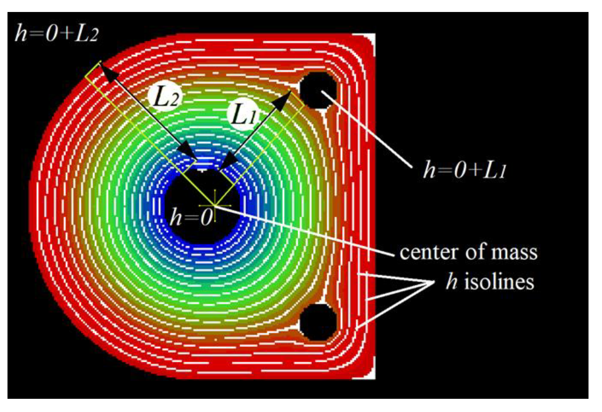
  18. Hong, X.; Xiao, G.; Zhang, Y.; Zhou, J. A new path planning strategy based on level set function for layered fabrication processes. Int. J. Adv. Manuf. Technol. 2022, 119, 517–529. [Google Scholar] [CrossRef]
  19. Le Dret, H.; Lucquin, B. The Finite Difference Method for Elliptic Problems. In Partial Differential Equations: Modeling, Analysis and Numerical Approximation; International Series of Numerical Mathematics; Birkhäuser: Cham, Switzerland, 2016; Volume 168. [Google Scholar] [CrossRef]
  20. Herman, E.; Strang, G. Calculus. Volume 3; OpenStax: Houston, TX, USA, 2016. [Google Scholar]
  21. Zhang, C.; Sun, P. Heuristic Methods for Solving the Traveling Salesman Problem (TSP): A Comparative Study. In Proceedings of the 2023 IEEE 34th Annual International Symposium on Personal, Indoor and Mobile Radio Communications (PIMRC), Toronto, ON, Canada, 5–8 September 2023; pp. 1–6. [Google Scholar] [CrossRef]
  22. Kadyrova, G.R. Intelligent Systems; Ul’anovsk State Technical University: Ul’anovsk, Russia, 2017. [Google Scholar]
  23. Fuchs, C.; Baier, D.; Semm, T.; Zaeh, M.F. Determining the machining allowance for WAAM parts. Prod. Eng. Res. Devel. 2020, 14, 629–637. [Google Scholar] [CrossRef]
  24. Soh, G.S.; Oh, X.Y. Wire Arc Additive Manufacturing Stepover Optimization based on Varying-Ratio Flat-Top Overlapping Model. In Proceedings of the 9th International Conference of Asian Society for Precision Engineering, Nanotechnology (ASPEN 2022), Singapore, 15–18 November 2022; Sharon, N.M.L., Kumar, A.S., Eds.; [Google Scholar] [CrossRef]
  25. Yanenko, N.N. The Method of Fractional Steps: The Solution of Problems of Mathematical Physics in Several Variables; Springer: Berlin/Heidelberg, Germany, 1971. [Google Scholar]
Figure 1. Deviation of layer height at the initial and final sections of formation: (a) photographs of typical multilayer thin walls; (b) schematic representation in section.
Modelling 05 00105 g001
Figure 3. Graphical view of the solution of the boundary value problem for h(x,y).
Modelling 05 00105 g003
Figure 4. Illustration of defining a destination point with coordinates xn, yn: (a) formation of a bead with constant h value; (b) transition to the next layer of the contour (the direction is chosen so that there is no overlap with the deposited bead, and the change in h value is minimal).
Modelling 05 00105 g004
Figure 5. The results of planning the welding path with the calculation of the temperature (°C) distribution for different moments of time: (a) 0.5 s; (b) 62 s; (c) 124 s; (d) 186 s; (e) 248 s; (f) 310 s; electron beam surfacing process photo (g); and the section deposited on the ELA-15I electron-beam installation (h).
Modelling 05 00105 g005
Figure 6. Computational results of trajectory planning for sections with no geometric similarity between the inner and outer boundaries: (a) section from Figure 4 with a rectangular hole; (b) section considered in [16]; (c,d) experimental trajectories of the electron beam movement on the surface of AISI 316L steel plate, treated without feeding filler wire.
Modelling 05 00105 g006
Table 1. Parameters of path planning simulation.
ParameterDescriptionValueUnit
Xlayer size along x-axis0.2m
Ylayer size along y-axis0.2m
hcoordinate step0.001m
Δttime step0.5s
rbsurfacing spot radius0.004m
steppath planning step0.0068m
λheat conductivity30W/(m·K)
cspecific heat450J/(kg·K)
ρdensity7800kg/m3
pheat source power800W
reffheat source effective radius0.003m
soverlapoverlap area fraction0.35-
Disclaimer/Publisher’s Note: The statements, opinions and data contained in all publications are solely those of the individual author(s) and contributor(s) and not of MDPI and/or the editor(s). MDPI and/or the editor(s) disclaim responsibility for any injury to people or property resulting from any ideas, methods, instructions or products referred to in the content.

