Article

Finite Element In-Depth Verification: Base Displacements of a Spherical Dome Loaded by Edge Forces and Moments

by
Vasiliki G. Terzi
* and
Triantafyllos K. Makarios
Institute of Structural Analysis and Dynamics of Structures, School of Civil Engineering, Aristotle University of Thessaloniki, 56124 Thessaloniki, Greece
*
Author to whom correspondence should be addressed.
Modelling 2024, 5(1), 37-54; https://doi.org/10.3390/modelling5010003
Submission received: 24 November 2023 / Revised: 12 December 2023 / Accepted: 19 December 2023 / Published: 21 December 2023

Abstract

:
Nowadays, engineers possess a wealth of numerical packages in order to design civil engineering structures. The finite element method offers a variety of sophisticated element types, nonlinear materials, and solution algorithms, which enable engineers to confront complicated design problems. However, one of the difficult tasks is the verification of the produced numerical results. The present paper deals with the in-depth verification of a basic problem, referring to the axisymmetric loading by edge forces/moments of a spherical dome, truncated at various roll-down angles, φ o . Two formulations of analytical solutions are derived by the bibliography; their results are compared with those produced by the implementation of the finite element method. Modelling details, such as the finite element type, orientation of joints, application of loading, boundary conditions, and results’ interpretation, are presented thoroughly. Four different ratios of the radius of curvature, r and shell’s thickness, and t are examined in order to investigate the compatibility between the implementation of the finite element method to the “first-order” shell theory. The discussion refers to the differences not only between the numerical and analytical results, but also between the two analytical approaches. Furthermore, it emphasizes the necessity of contacting even linear elastic preliminary verification numerical tests as a basis for the construction of more elaborated and sophisticated models.

1. Introduction

Nowadays, designers have the ability to implement various numerical methods in order to study an engineering problem. Sophisticated numerical models are produced by utilizing elaborated finite element types, laws of materials, analysis types, and loading and boundary conditions. However, the major difficult task is twofold and regards the process of the validation and verification of the numerical models, which acquires a particular significance [1]. In particular, the validation is related to the physics of the problem or otherwise, namely the correctness of the mathematical equations constructed for modeling certain mechanical phenomena. Furthermore, the verification is related to the correctness of the solution of the assumed approximation [2] or otherwise, namely the level of confidence that an approximate result corresponds to a given tolerance range of the exact solution of the mathematical model [3]. The aforementioned processes can be fulfilled by a comparison of the numerical results to laboratory/in situ experimental or analytical results [4,5].
The construction of shells, such as roofs of industrial buildings, pressure vessels, nuclear reactors, sports centers, and auditoriums, has been expanded in recent years, since they combine practical, functional, cost-effective, and aesthetic needs [6,7,8]. Among shells’ structures, rotationally symmetric domes are frequently designed not only due to their small mass and high stiffness, but also due to their attractive architectural forms [9]. One of the principal modeling aspects that the designer faces is the decision of performing a “thin”/“thick” shell or fully three-dimensional analysis.
The theory of thin-walled shells is based on fundamental assumptions, which allows the efficient analysis of shell structures to be conducted in the two-dimensional rather in the three-dimensional space [10,11]. The “thin” or “first-order” plate/shell theory, which is also known as the “Kirchhoff-Love” theory [12,13,14,15], is fοunded on the following assumptions [16]: (i) normals to the shell mid-surface remain straight and normal after deformation; (ii) the transverse normal stress is negligible (Figure 1a). Additional simplifications refer also to the following assumptions: (i) the strains receive very small values compared with unity [17,18]; (ii) the shell thickness remains constant. On the other hand, the “thick” or “second-order” plate/shell theory, which is also known as the “Mindlin-Reissner” theory, takes transverse shear deformation into account; therefore, the normals to the shell mid-surface do not remain normal after deformation (Figure 1b) [19,20]. As a general comment, it could be stated that the “first-order” and “second-order” plate/shell theories are the analogies of Euler–Bernoulli [21] and Timoshenko–Ehrenfest [22,23] beam theories, respectively [24].
The first question that arises is regarding the criteria under which the engineer will perform an analysis by the implementation of shell finite elements by applying the “first-order” or the “second-order” theory. Furthermore, an additional question that arises regards the criteria for the conduction of a full three-dimensional analysis by the implementation of solid finite elements. Both answers depend on the physics and geometric nature of the problem under study. However, Vlassov, in 1958 [25], proposed that the limit ratio between the radius of curvature, r , and the shell’s thickness, t , for the application of the “thin” shell theory, receives the value of r / t = 30. In 1959, Timoshenko and Woinowsky-Krieger proposed that if the shell’s thickness, t , is comparable to its radius of curvature, r , then the “second-order” theory should be applied or even a three-dimensional analysis should be conducted [26]. Additionally, in 1975, Flügge proposed that the “first-order” theory produces rigorous results in the case of the shell’s thickness, t , which is small [27] and is almost the same as the criterion of r / t 1, proposed by Brush and Almroth [17]. In 1977, Heyman defined the limit ratio for the application of the “thin” shell theory as r / t > 20 [28]. Moreover, in 1983 and 1985, Calladine and Bushnell [15,16], respectively, defined the aforementioned limit ratio as r / t = 10.
The behavior of “thin” or “thick” shells under various loading conditions can be studied by a number of the available approaches: analytical [29,30,31,32]; a combination of analytical and numerical [33,34,35,36]; a combination of analytical, experimental, and numerical [37,38,39,40]; semi-analytical [41,42,43].
The development and evolution of numerical methods have limited the utilization of “thin” shell theory [3]. However, the comparison between analytical and numerical results remains a challenging task. The most characteristic case is the Girkmann problem [44], which refers to the behavior of a concrete spherical dome that is stiffened by a foot ring under a dead gravity load. The verification challenge was posed in 2008 by the International Association of Computational Mechanics (ICAM) to the finite element community [45]. Different models and formulations were implemented during various verification processes [3,46,47,48].
The behavior of the shell is a combination of the membrane and bending theory. The membrane theory is valid only in shell regions that are sufficiently distant from supports; concentrated loads; geometrical discontinuities, such as shell thickness; slope; curvature [49,50,51]. In all of the aforementioned cases, membrane theory provides adequate solutions to each problem [52]. The present paper deals with a case of edge loading, which, even though it is a basic problem, has been poorly investigated. In particular, it refers to the in-depth verification of the implementation of the finite element method considering a basic problem of a spherical dome’s behavior. The shell structure is loaded along its perimeter by edge horizontal forces and moments. The basic asset of the present paper is that two analytical formulations are derived by the bibliography, characterized as the first and second approximation, which refer to the determination of the base’s translational and rotational displacements. Therefore, the necessary comparisons are performed between the results of the two analytical approaches. Fundamental aspects of the finite element modeling are investigated and discussed in detail, such as: the finite element type, mesh discretization, orientation of the joint coordinate system, the loading application, boundary conditions, and results’ interpretation. In order to determine the limits of the application of the “thin” shell assumption, four different ratios r / t are taken into account. The numerical results are compared with the analytical ones. Both the convergence and differences are discussed in detail and are attributed to certain modeling aspects or theoretical assumptions.

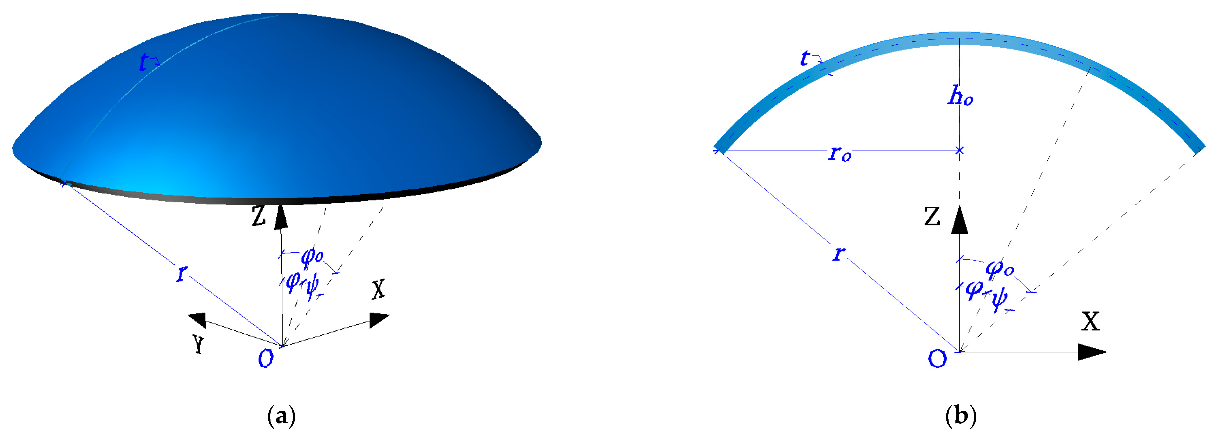
2. Theoretical Background

Consider the spherical dome of radius, r , and thickness, t , which is truncated at a roll-down angle, φ o , increasing in clock-wise way (Figure 2). The circumference of the spherical cap is characterized by the radius, r o , and by the corresponding height, h o . The dome’s material is considered as an isotropic linear elastic and is characterized by Young’s modulus, E , and Poisson’s ratio, v .
Figure 3 depicts the forces and moments which develop according to the membrane and bending theory of shells [26]. The forces Ν φ , Ν θ , and N φ θ = Ν θ φ form the basis of the membrane theory. The moments M φ , M θ , and M φ θ = M θ φ , in combination with the transverse shear forces Q φ and Q θ , form the basis of the bending theory.
The bending behavior of the spherical shell is described by the two approximated equations proposed by Geckeler J.W. [53].
d 2 Q φ d φ 2 + c o t φ · d Q φ d φ + c o t 2 φ ν · Q φ = Ε · t · V
d 2 V d φ 2 + c o t φ · d V d φ + c o t 2 φ + ν · V = r 2 · Q φ D
where V is the rotation of a tangent to a meridian; and D = E · t 3 / 12 · 1 v 2 . The shear force, Q φ , receives the following form.
Q φ = e β · φ s i n φ · C 1 · c o s β · φ + C 2 · s i n β · φ
where
β 4 = 1 v 2 4 · 1 + 12 · r 2 t 2
In the case of very thin shells and for large values of angle φ , both Q φ and V are damped out rapidly as the distance from the edge increases. Furthermore, in the case of thin shells, according to Equation (3), β receives large values and the first derivative of Q φ is large in comparison with Q φ . Moreover, the second derivative of Q φ is large in comparison with the first derivative of Q φ . The aforementioned conclusions enable us to proceed with the approximation of neglecting the functions Q φ and V , as well as their first derivatives in the left part of Equation (1). Therefore, Equation (1) receives the following form.
d 2 Q φ d φ 2 = Ε · t · V
d 2 V d φ 2 = r 2 · Q φ D
Finally, the general solution of the shear force, Q φ , is given by Equation (5).
Q φ = C 1 · e λ · φ · c o s λ · φ + C 2 · e λ · φ · s i n λ · φ + C 3 · e λ · φ · c o s λ · φ + C 4 · e λ · φ · s i n λ · φ
where
λ 4 = 3 · 1 v 2 · r t 2
Two cases of edge conditions along the dome’s perimeter are taken into account: (i) base force, H o ; (ii) base moment, M o (Figure 4). The edge force, H o , causes the horizontal translation Δ H , H ο and the rotation Δ φ , H ο of the base. Furthermore, the edge moment, M o , causes the horizontal translation Δ H , M ο and the rotation Δ φ , M ο of the base.
In the case that the aforementioned two loading types are imposed on the shell’s edge and no hole exists at the top, Equation (5) can be simplified, as follows:
Q φ = C 1 · e λ · φ · c o s λ · φ + C 2 · e λ · φ · s i n λ · φ
Q φ = C · e λ · φ · s i n λ · ψ + γ
Therefore, for each loading type, two boundary conditions suffice in order to solve Equation (7a) in terms of C 1 , C 2 or Equation (7b) in terms of C , γ . For the horizontal edge force, H o , the boundary conditions are described by Equation (8), while for the edge moment, M o , they are described by Equation (9). In particular, the horizontal force, H o , which is applied at the edge, φ ο , produces only N φ types of forces (Equation (8b)) and no edge moments, M φ (Equation (8a)). Furthermore, the moment M ο , which is applied at the edge, φ ο , produces only M φ moments (Equation (9a)) and no edge N φ type of forces (Equation (9b)).
M φ φ = φ ο = 0
Ν φ φ = φ ο = H ο · c o s φ ο
M φ φ = φ ο = M ο
Ν φ φ = φ ο = 0
Timoshenko and Woinowsky–Krieger [26] provide, as a first approximation, Equation (10), in order to determine the dome’s base displacements under various values of the roll-down angle, φ o . The first observation is that the rotation, due to the edge force, H o (Equation (10b)), equals to the translation due to the edge moment, M o (Equation (10c)), due to the reciprocity theorem, and under the assumption that H o = M o , since H o and M o , which are applied at the edge circumference of the dome, receive the same values expressed in kN/m or kNm/m, respectively.
The second observation refers to the rotation due to the edge moment, M o (Equation (10d)). In particular, Δ φ , M o is independent of the roll-down angle, φ o and corresponds to a fixed value.
Δ H , H o = 2 · r · λ · s i n φ o 2 E · t · H o
Δ φ , H o = 2 · λ 2 · s i n φ o E · t · H o
Δ H , M o = 2 · λ 2 · s i n φ o E · t · M o
Δ φ , M o = 4 · λ 3 E · r · t · M o
Hetényi M., in 1937/1938, provided a closer approximation to the determination of the dome’s base displacements, described by Equation (1) [54]. In particular, the following new variables were introduced.
Q 1 = Q φ · s i n φ
V 1 = V · s i n φ
The quantities Q φ and V are substituted in Equation (1); by applying the aforementioned procedure, the shear force is given by Equation (12).
Q φ = C · e λ · ψ s i n φ ο ψ · s i n λ · ψ + γ
The two unknowns, C , γ , are determined by the application of the boundary conditions that are described in Equations (7) and (8) and correspond to the two loading types. Finally, the equations of the displacements, according to Hetényi’s approach, are described by the following:
k 1 = 1 1 2 · v 2 · λ · c o t φ o
k 2 = 1 1 + 2 · v 2 · λ · c o t φ o
Δ H , H o = r · λ · s i n φ o 2 E · t · k 2 + 1 k 1 · H o
Δ φ , H o = 2 · λ 2 · s i n φ o E · t · k 1 · H o
Δ H , M o = 2 · λ 2 · s i n φ o E · t · k 1 · M o
Δ φ , M o = 4 · λ 3 E · r · t · k 1 · M o
The comparison between Equations (10) and (13) leads to the conclusion that according to the second analytical approach, the rotation due to the edge moment, M o (Equation (13f)), depends on the roll-down angle, φ o , through the value of the k 1 parameter (Equation (13a)).

3. Finite Element Approach

Consider a spherical dome of the radius, r = 25 m, which is subjected to the edge force, H o = 1 kN/m, and edge moment, M o = 1 kNm/m, along its perimeter. In order to investigate the behavior of the “thin” shell finite element, four different cases of ratios r / t are taken into account: (i) 1000, (ii) 500, (iii) 100, and (iv) 30. The first three ones definitely belong to the range of “thin” shells, while the fourth one belongs to the transitional area of the definition between “thin” and “thick” shells. The roll-down angle, φ o , receives different values ranging from 5° to 90° by a step of 5°. The Young’s modulus of the concrete material equals to E = 33 GPa and the Poisson’s ratio equals to v = 0.15. All that is necessary for the calculations’ data are presented in Table 1.

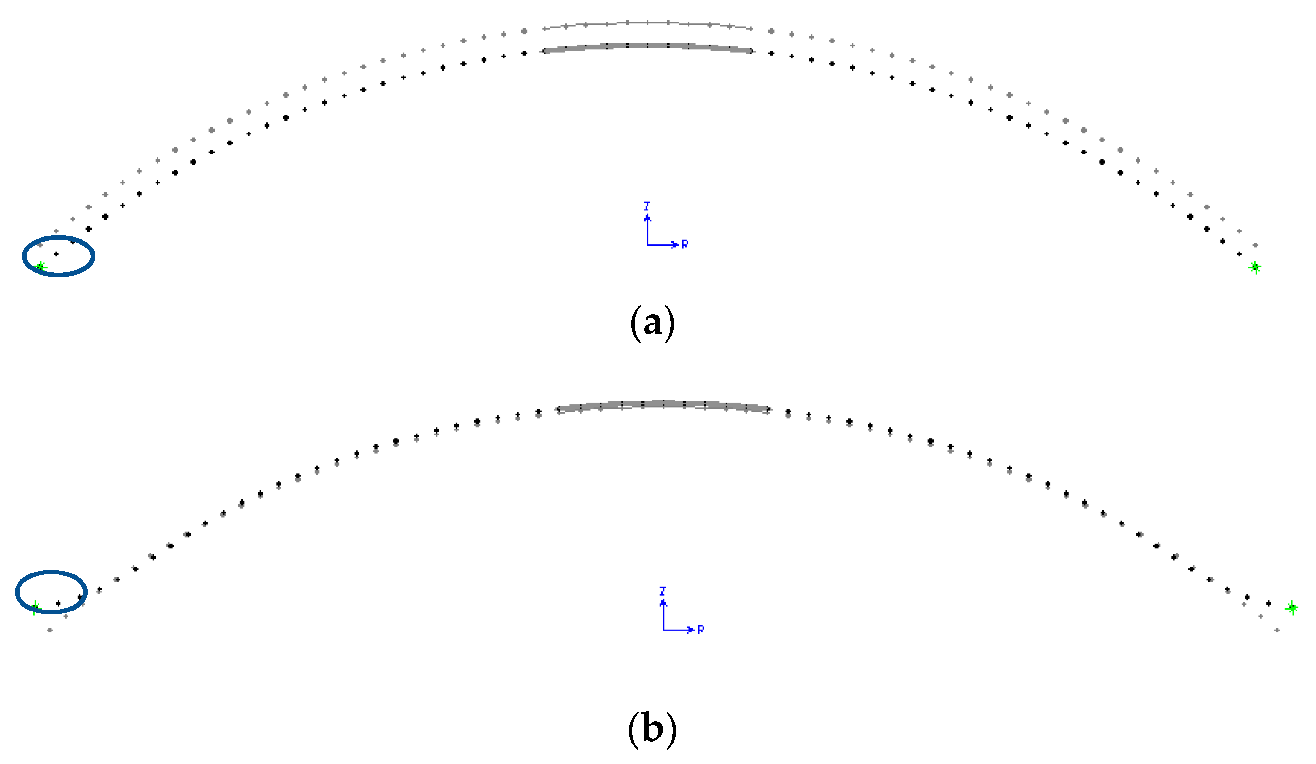
3.1. Finite Element Modelling

The present section covers some of the basic modeling aspects, such as: (i) the finite element type; (ii) model discretization; (iii) orientation of the joint local coordinate system; (iv) loading definition; (v) boundary conditions; (vi) results’ interpretation. The finite element software applied for the analyses is SAP2000v.24 [55].

3.1.1. Finite Element Type

The homogeneous shell element, provided by SAP2000v.24, is implemented, since it combines independent membrane and plate behavior. Once the element is warped (non-planar), these behaviors become coupled. The isoparametric formulation is used by the membrane behavior, which includes both translational in-plane stiffness components and a “drilling” rotational stiffness in the direction normal to the plane of the element [56,57]. Two-way, out-of-plane, plate rotational stiffness components and a translational stiffness component in the direction normal to the plane of the element are included in the plate-bending behavior. The thin-plate or otherwise stated as the Kirchhoff formulation, which neglects the transverse shearing deformation, is chosen in order to achieve the compatibility between the numerical and analytical results. All the in-plane displacements are quadratic and all the out-of-plane displacements are cubic.
Figure 5 depicts the forces and moments, which develop in a typical shell element of SAP2000v.24 (grey colored). Each shell element possesses a local coordinate system denoted by 123 axes. The dashed line in the middle of its thickness corresponds to the mid-surface. Forces F 11 ,   F 22 , and F 12 correspond to the membrane theory, while forces V 13 and V 23 are the transverse shear forces that correspond to the bending theory. Furthermore, moments M 11 ,   M 22 , and M 12 also correspond to the bending theory. Both forces and moments are expressed in kN/m and kNm/m, respectively.
The analogy between the numerical and theoretical definitions of the forces’ and moments’ parameters is described as follows: F 11 = N θ ; F 12 = N θ φ ; V 13 = Q θ ; F 22 = N φ ; V 23 = Q φ ; M 11 = M θ ; M 12 = M θ φ ; and M 22 = M φ .

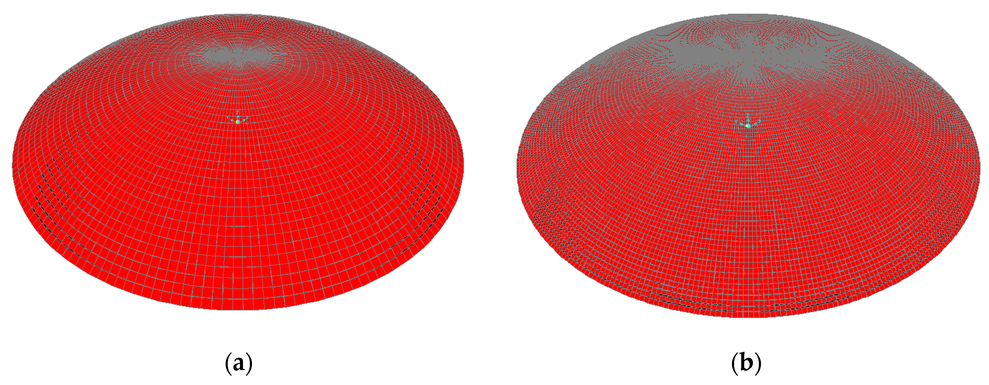
3.1.2. Model Discretization

The density and the number of finite elements in a model are of primary importance. The finite element mesh is produced automatically by the software, once certain values of the following geometry parameters are inserted: the radius of the spherical dome, r ; roll-down angle, φ ο ; angular number of divisions; and number of divisions along height, h o . Special attention was given to the determination of the number of divisions. In particular, the discretization along the perimeter of the truncated spherical dome and along the height of the spherical cap must produce shell elements characterized by almost equal dimensions along the meridian and circumferential direction. The perimeter of the spherical cap equals to L o = 2 · π · r o . The dimension of the base finite elements along the perimeter equals to l f . e . , p e r . = L o / n . o . d p e r . , where n . o . d p e r . is the number of divisions along the perimeter. The height of the spherical cap equals to h o = r r o / t a n φ ο . Therefore, the number of divisions along the height is determined by the ratio, n . o . d h e i g h t . = h o / l f . e . , p e r . .
In order to investigate the discretization effects on the numerical results, two different schemes were formulated: (i) coarse and (ii) dense mesh. Specifically, in the case of the coarse mesh discretization, the perimeter of the spherical cap of radius, r o , is divided into sections corresponding to an angle of 2°, while in the case of the dense mesh discretization, the aforementioned angle receives a value of 1°. Both discretization schemes lead to a high concentration of strains and stresses at the top of the spherical dome due to the high number of meridians that pass through. However, taking into account that the loading is not applied at the top but at the edges of the truncated spherical dome, and that the target is the estimation of the base displacements, the discretization effects at the top of the dome are considered to be not only local but negligible as well. In the case that the loading passes through the top of the dome, such as gravitational loading, or is applied exactly at the aforementioned point, as a concentrated force/moment, then the engineer should seek a different discretization scheme that lacks a node at this geometrical point. Furthermore, in order to achieve the optimum stress distribution, the mesh should be characterized by symmetry. Figure 6 depicts the two mesh formulations, which correspond to a spherical dome of a roll-down angle, φ o = 40°.

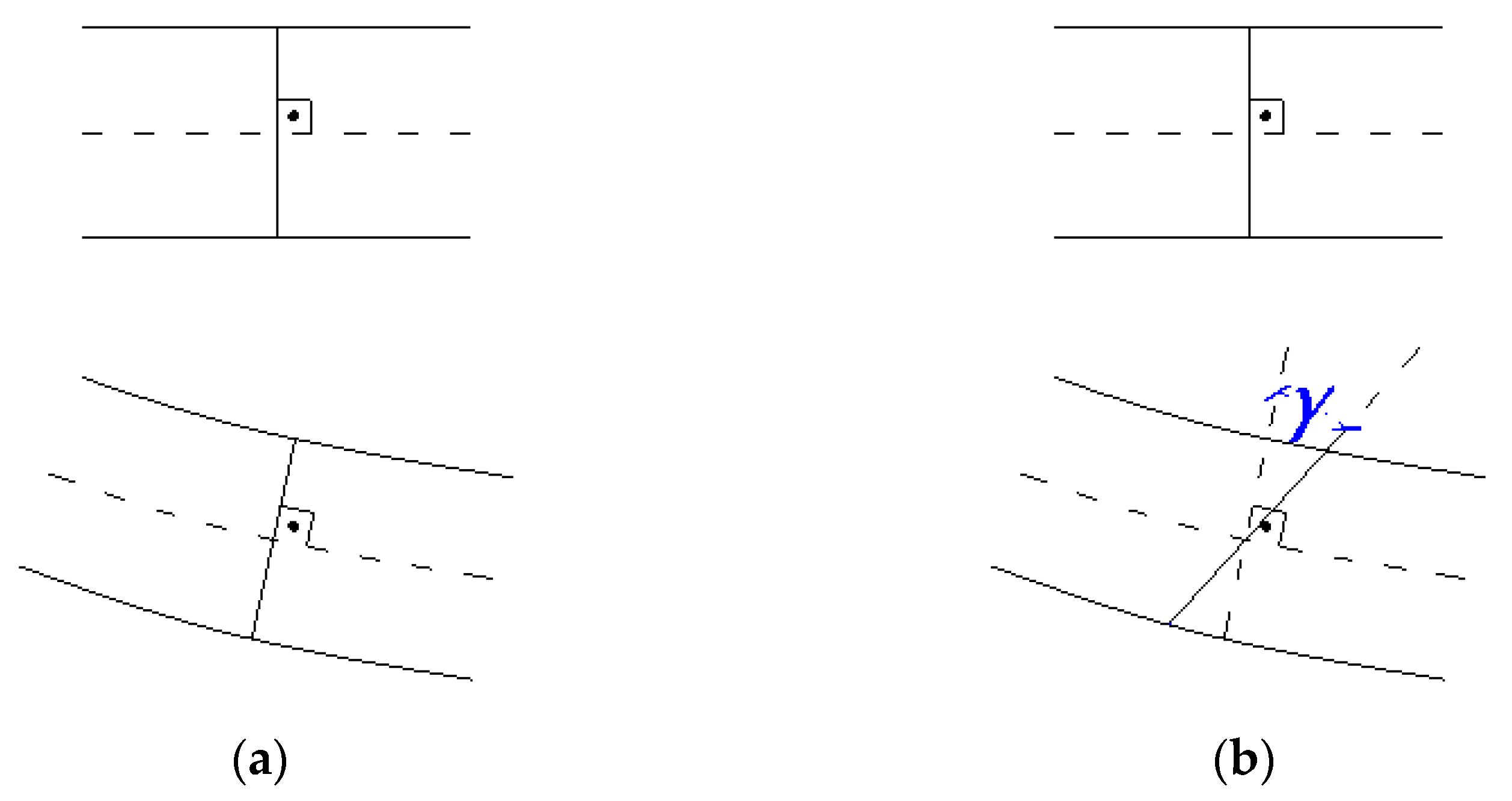
3.1.3. Orientation of Joint Local Coordinate System

The joint local coordinate system is denoted as 123 in SAP2000 and coincides with the global coordinate system, XYZ. However, in order to achieve compatibility with the theoretical definitions, the local coordinate of the base joints is rotated around the: (i) Z and (ii) Y axis. The first rotation causes the local axis 1 to pass through the center of the spherical cap, while the second rotation causes the local axis 1 to pass through the center of the sphere. In this way, the local axis 3 is always tangential to the shell’s mid-surface, and the local axis 2 is perpendicular to the plane defined by local axes 1 and 3. Figure 7a depicts the final orientation of the joint local coordinate system in a typical cross-section, and Figure 7b depicts a typical rotated finite element of one of the created numerical models. The purple lines correspond to the bounding box of the finite element, while the grey plane corresponds to the shell’s mid-surface. The red, white and cyan axes located at the mid-surface of the finite element correspond to local axes 1, 2, and 3, respectively. Axes 1 and 2 belong to the mid-plane, while axis 3 is perpendicular to it. Therefore, in correlation to Figure 5 (forces and moments), forces F 11 = N θ develop along the red axis, while forces F 22 = N φ develop along the white axis. Furthermore, the red, white, and cyan axis axes located at the four nodes of the finite element correspond to local axes 1, 2, and 3, respectively.

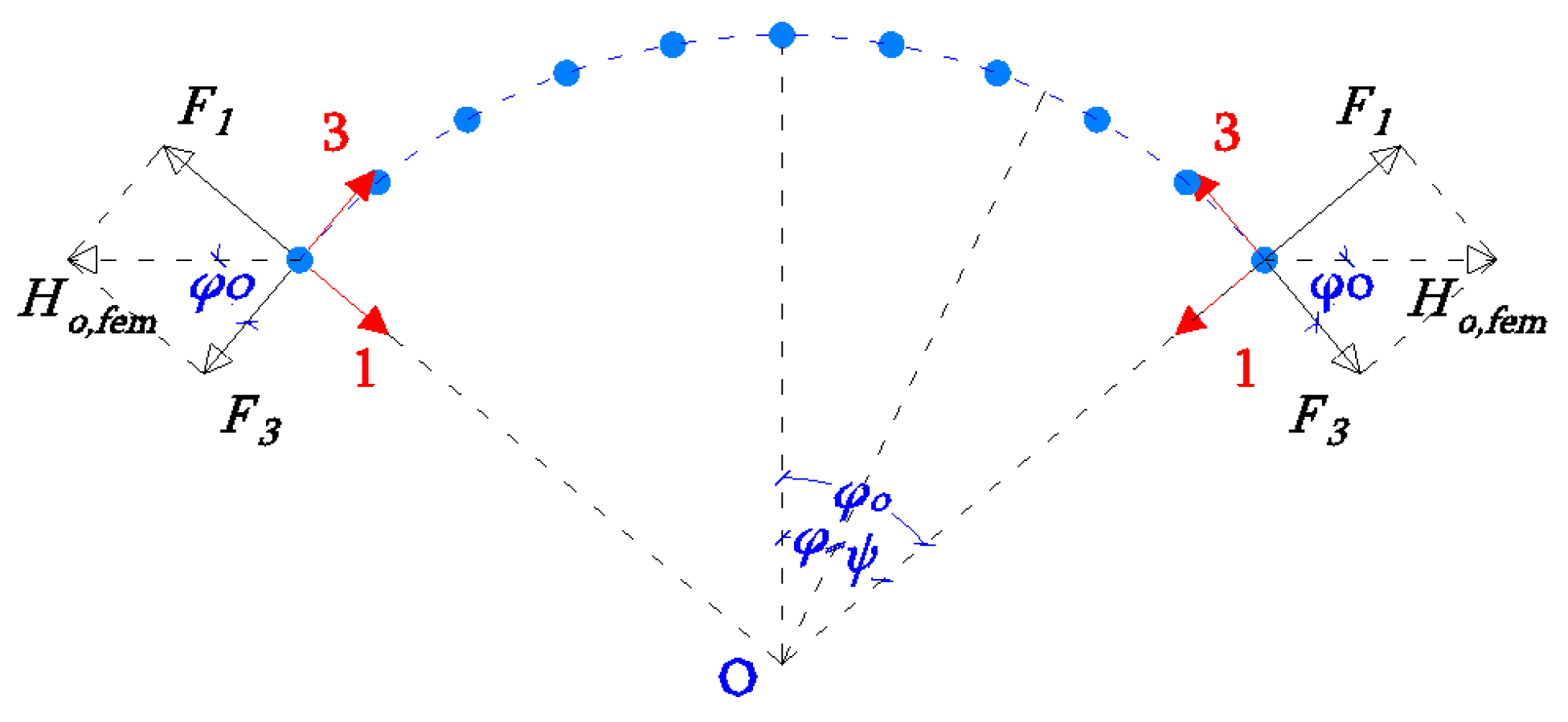
3.1.4. Loading Definition

According to the theory, the edge horizontal force receives the value of H o = 1 kN/m, and the edge moment receives the value of M o = 1 kNm/m. Therefore, in the finite element model, the horizontal force receives the value of H o , f e m = H o / n . o . n . and the moment receives the value of M o , f e m = M o / n . o . n . , where n . o . n . corresponds to the number of nodes that belong to the perimeter of the spherical cap, according to each mesh discretization formulation. The loading is assigned as joint load (forces and moments). The value of the edge moment M o , f e m is assigned to local axis 2 of the base joints. Furthermore, in the case of the horizontal load application, the edge force H o , f e m is analyzed in two components along the joint local axes 1 and 3 by the application of Equation (14).
F 1 = H o , f e m · s i n φ ο
F 3 = H o , f e m · c o s φ ο
Figure 8 depicts the appropriate geometry for the definition of application of the horizontal edge load, H o , f e m .
.

3.1.5. Boundary Conditions

Each joint of the homogeneous shell element corresponds to six degrees of freedom: three translational along local axes 1, 2, and 3; and 3 rotational about local axes 1, 2, and 3. In order to achieve compatibility with the theoretical assumptions, the translation along local axes 1 and 3, as well as the rotation around local axis 2 is unrestrained. More specifically, according to the first load case which corresponds to the application of edge force, H o , the base nodes are free to translate along local axes 1 and 3 and to rotate around local axis 2. The same also issues to the second load case, which corresponds to the application of the edge moment, M o , around local axis 2.

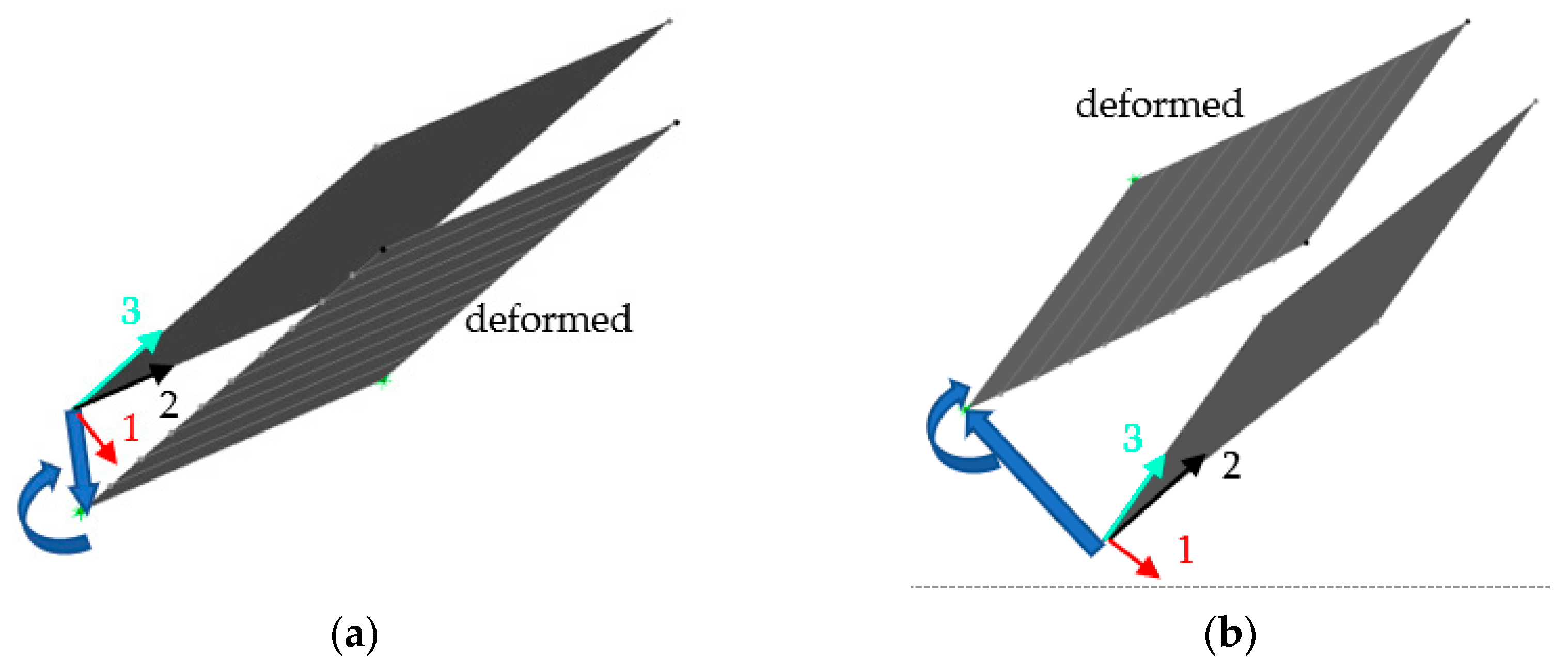
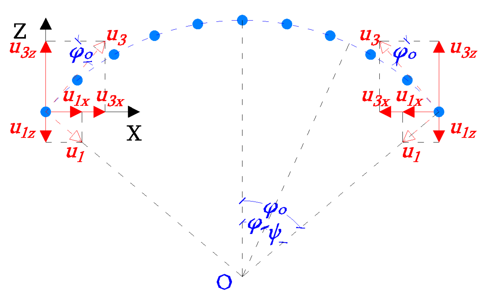
3.1.6. Results’ Interpretation

Figure 9 depicts the deformation of a typical shell element that belongs to the perimeter/base of the truncated spherical dome under the application of horizontal edge force, H , o and edge moment, M o . Under both types of loading, the base points translate along local axes 1 and 3 and rotate about local axis 2.
The terms Δ φ , H o and Δ φ , M o correspond to the rotational displacement caused by the horizontal edge force, H o , and edge moment, M o , respectively. Therefore, in the framework of the finite element method, the aforementioned rotational displacements correspond to the rotation of the base joints around local axis 2, according to the loading definition. Furthermore, the terms Δ H , H o and Δ H , M o correspond to the horizontal displacement caused by the horizontal edge force, H o , and edge moment, M o , respectively. Hence, the translational joint displacements along local axes 1 and 3 must be analyzed along global coordinate axes X and Z, in order to determine the horizontal displacement (Figure 10).
The theoretical term is expressed by Equation (15).
Δ H , i = u 1 x + u 3 x = u 1 · s i n φ ο + u 3 · c o s φ ο

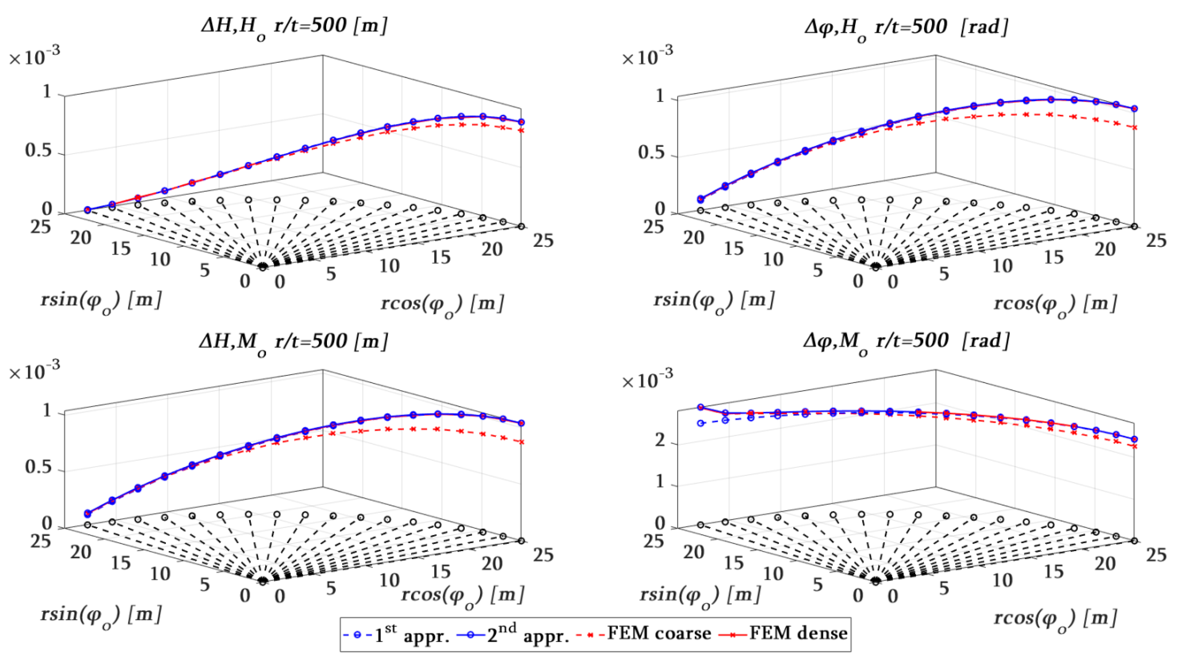
3.2. Comparison between Analytical and Numerical Results

Figure 11 depicts the typical deformation of a cross-section of the truncated spherical dome under the action of both types of loading. The grey dots represent the initial position of the finite element nodes, while the black dots represent the final deformed shape, after the application of loading. The horizontal edge force, H o , affects the deformed shape of the spherical dome in total, while in the case of the edge moment, M o , the deformation is more locally pronounced near the edge. Due to the symmetry of the loading and the structural geometry, as well, the results of the numerical analyses, either in terms of stresses or displacements, at any cross-section in the r -Z plane, are the same. Therefore, only the base displacements of the point which belongs to Χ = r , Z = 0, and ψ = φ ο are extruded from the results’ data base.
Figure 12, Figure 13, Figure 14 and Figure 15 depict the comparison diagrams between the results of the theoretical and numerical analyses for the four ratios of r / t . In particular, the blue dashed line corresponds to the analytical results according to the first approach (Equation (10)), while the blue continuous line corresponds to the analytical results according to the second approach (Equation (13)). Moreover, the red dashed line corresponds to the numerical results under the assumption of a coarse mesh discretization, while the continuous one is under the assumption of a dense mesh discretization. Each black dashed line depicted in the XY plane of the 3D diagrams corresponds to the radius of the spherical cap from a roll-down angle from 5° to 90°.
Figure 12 depicts the results of a very thin shell, which is characterized by r / t = 1000. The two analytical approaches coincide, except in the case of the rotational displacement due to edge moment loading, Δ φ , M o , and for small values of roll-down angles. The aforementioned difference is attributed to the dependence of the rotation on trigonometric terms of the roll-down angle, according to the second theoretical approach. The existence of the trigonometric term k 1 (Equation (13a)), in the denominator of Δ φ , M o (Equation (13f)), alters the analytical results for small values of φ ο . Furthermore, the difference between the coarse and dense finite element formulation is obvious for large numbers of roll-down angles for all degrees of freedom and under both loading cases. On the contrary, for small values of roll-down angles, the coarse discretization scheme suffices and converges to the second theoretical approach. The aforementioned can be explained by the fact that at small values of φ ο , the radius of the spherical cap, r o and consequently, the perimeter of the spherical cap, L o , receives small values. Therefore, taking into account the small thickness, t , the selection of the discretization at 1° or 2° angles is meaningless.
Therefore, in the case of very thin shells characterized by r / t = 1000, the following two cases can be distinguished: (i) large values of roll-down angles, φ ο 20°, at which a dense mesh discretization scheme must be applied; (ii) small values of roll-down angles, φ ο < 20°, at which a coarse mesh discretization scheme suffices.
Figure 13 depicts the results of a very thin shell, which is characterized by r / t = 500. Both translational and rotational displacements receive smaller values than the case of r / t = 1000. The results of the two analytical approaches coincide, except in the range of small values of roll-down angles ( φ ο < 20°) for rotational displacements under the application of edge moments, Δ φ , M o . The discrepancy between the results of a coarse and a dense finite element discretization mesh are prominent for large values of roll-down angles ( φ ο 30°), for all the degrees of freedom. The dense finite element mesh provides the best coincidence with the results of the second theoretical approach. However, it has to be pointed out that the coarse finite element mesh also produces excellent results for Δ φ , M o in the range of small values of roll-down angles.
Therefore, in the case of very thin shells characterized by r / t = 500, the following two cases can be distinguished: (i) large values of roll-down angles, φ ο 30°, at which a dense mesh discretization scheme must be applied; (ii) small values of roll-down angles, φ ο < 30°, at which a coarse mesh discretization scheme suffices.
Figure 14 depicts the results of a thin shell, which is characterized by r / t = 100. All four approaches are in excellent coincidence, except for the case of the smallest roll-down angle, which equals 5°. Furthermore, the difference between the two theoretical approaches regarding the term Δ φ , M o for small values of roll-down angles ( φ ο < 40°) remains characteristic. Therefore, in the case of thin shells characterized by r / t = 100, the finite element density discretization does not affect the results except in the case of φ ο = 5°.
Figure 15 depicts the results of a thin shell, which is characterized by r / t = 30 and belongs to the transitional area of the definition between “thin” and “thick” shells. The difference between the first and second theoretical approach is not only detected in Δ φ , M o terms but also in Δ φ , H o , which is equal to Δ H , M o in the range of roll-down angles less than 50°. Another interesting observation refers to the coincidence of the results between the coarse and dense finite element discretization. The aforementioned can be explained by the following. Taking into account that the dome’s thickness receives a large value ( t = r / 30 = 0.833 m), even the coarse mesh, which corresponds to an angle of 2°, can be considered as a dense one, which corresponds to an angle of 1ο. Furthermore, for all degrees of freedom, except the translational one, Δ H , H o , a great discrepancy can be noticed between the second theoretical approach and the finite element results in the small range of roll-down angles, φ ο 10°. The aforementioned is attributed to the fact that the dome can be considered as a “thick” shell but also as a “shallow” one as well.
Therefore, according to Figure 15, in the case of shells characterized by r / t = 30, the finite element density discretization does not affect the results. Furthermore, the discrepancy between the two theoretical approaches cannot be ignored for values of roll-down angles that are smaller than 50°.
The previous comparison of the results was performed optically. Since data already exist, the comparison can be also performed statistically. Therefore, in order to quantify the error according to the second (2nd) analytical approach, the Mean Average Error is implemented, which is described by Equation (16).
M P E = 100 % n · i = 1 n a i f i a i
where n is the number of samples and is equal to 18; a i is the value of displacements for each degree of freedom according to the second analytical approach; and f i is the corresponding value of displacements according to the three remaining approaches, which are regarding the first (1st) analytical approach, the coarse mesh finite element formulation, and the dense mesh finite element formulation. Table 2 presents the calculated Mean Average Errors for each one of the aforementioned cases.
The following observations can be made: (i) the increase in the ratio r / t results to an increase in the Mean Average Error for all the degrees of freedom and for all of the approaches; (ii) the Mean Average Error is the same for the all the approaches in the cases of the coupling terms, Δ φ , H o and Δ H , M o , since their values are the same for each roll-down angle, φ 0 ; (iii) the higher values of Mean Average Errors correspond to the coarse mesh finite element formulation except for ratios r / t equal to 100 and 30, at which the first analytical approach deviates from the solution of the second analytical approach for the Δ φ , M o degree of freedom; (iv) the smallest values of Mean Average Errors correspond to the dense mesh finite element formulation; (v) for the ratio r / t equal to 30, the coarse and dense finite element formulation produce results of the same quality.

4. Conclusions

The present paper refers to the in-depth verification of the application of the finite element method in order to determine the base displacements of a thin spherical dome, which is truncated for various roll-down angles under the action of edge horizontal forces and rotational moments. Some of the general basic conclusions are summarized in the following.
  • The validation and verification of finite element models implemented to study a specific engineering case are not only crucial but also of vast importance.
  • In the absence of laboratory or in situ experiments, the engineer should refer to the results of an analytical approach. The verified finite element model, even under the assumptions of linearity and elasticity, forms a stable basis for its evolution and development under non-linear assumptions.
  • Special attention should be given by the engineer on the assumptions by which an analytical approach is governed and on the appropriate available finite element tools.
  • The engineer must be fully conversant with the capabilities or restrictions of the available finite element software.
Furthermore, some of the conclusions derived by the specific problem under study are the following:
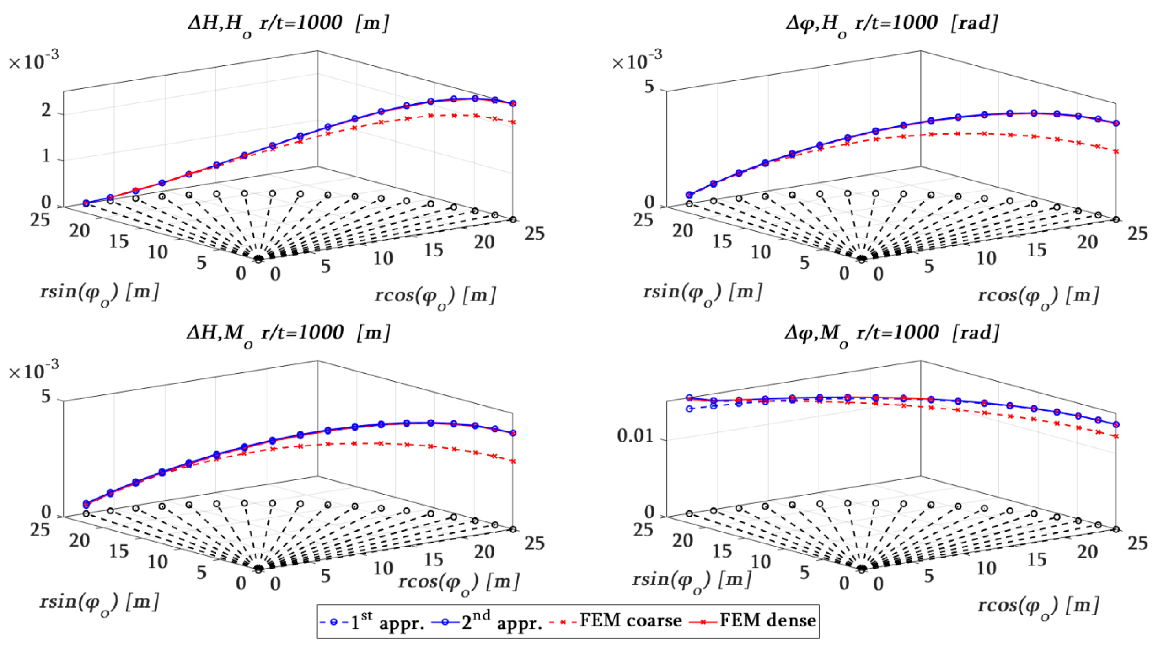
  • Two theoretical and analytical approaches have been implemented. The basic difference refers to the dependency of the rotational displacements caused by edge moments, on the value of the roll-down angle for all the considered values of the ratio, r / t .
  • As the ratio, r / t , becomes larger, or in other words, the shell becomes thicker, the discrepancy between the two analytical approaches is evident not only in rotational but also in translational displacements.
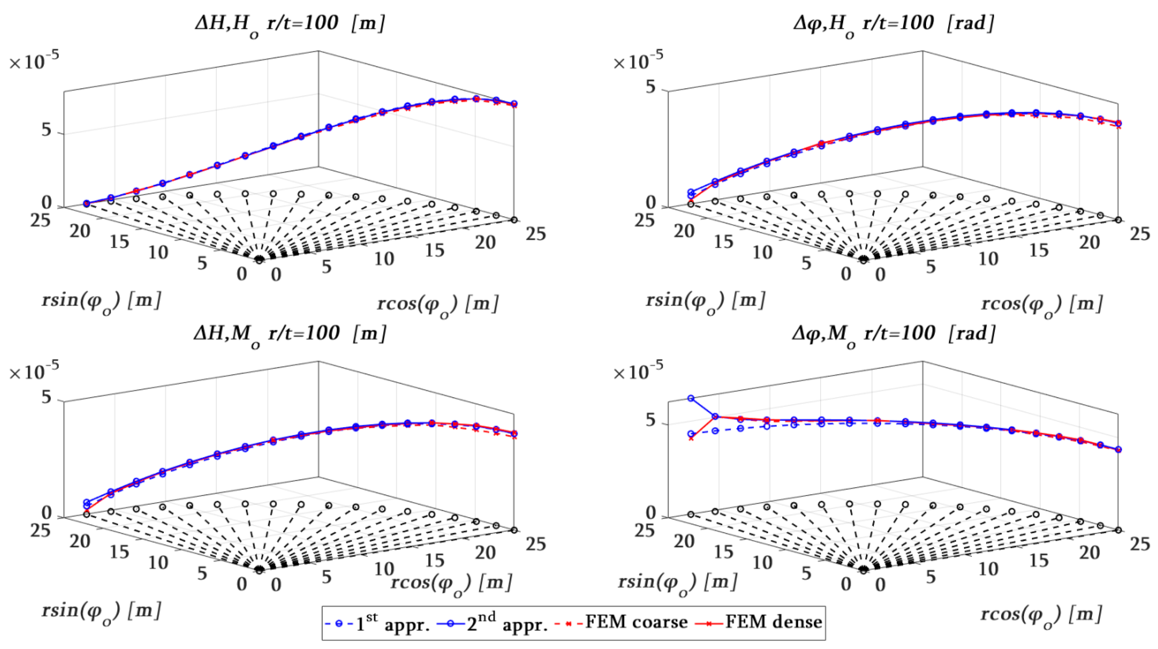
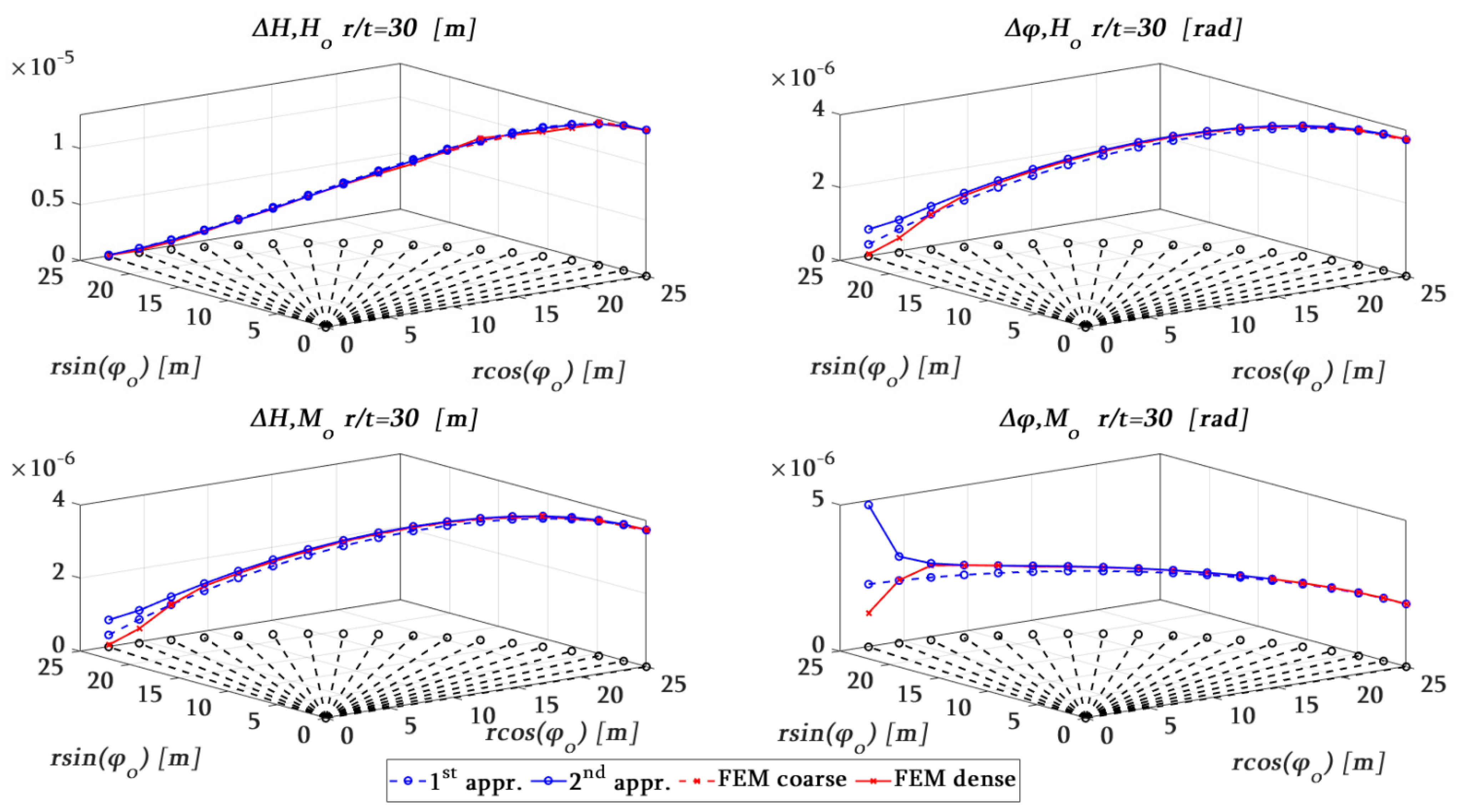
  • The numerical results considering the dense finite element discretization approach are in excellent agreement with the analytical ones derived by the second analytical approach for all ratios of r / t .
  • The effect of the finite element mesh discretization on numerical results is more pronounced in the case of very thin shells. In particular, for r / t 500 and for the roll-down angle φ o 30°, a dense mesh should be applied. On the contrary, as the shell thickness increases ( r / t 100), no difference between the coarse and dense mesh is detected.
  • Differences between the numerical and analytical results are detected for the case of r / t = 30, which belongs to the transitional area of definition between “thin” and “thick” shells but only in the range of small values of roll-down angles ( φ ο 10°). The behavior of the dome as a “thick shallow” shell cannot be captured by the implementation of homogeneous and thin shell elements. The use of the thick shell formulation or of three-dimensional finite elements is proposed.
  • According to the aforementioned conclusions, the main future research direction regards the finite element modeling of “thick shallow” shells by the use of three-dimensional elements.
In conclusion, the process of verification of the numerical models demands a thorough knowledge not only of the available software and its capabilities, but also on the physics of the case study, which can be derived by analytical solutions. Although, in most cases, the theoretical approach is usually based on assumptions that simplify the case study, a successful verification will form the basis for the development of more sophisticated numerical models.

Author Contributions

Conceptualization, V.G.T.; methodology, V.G.T.; software, V.G.T.; validation, V.G.T.; formal analysis, V.G.T.; investigation, V.G.T.; resources, V.G.T. and T.K.M.; data curation, V.G.T.; writing—original draft preparation, V.G.T.; writing—review and editing, V.G.T. and T.K.M.; visualization, V.G.T.; supervision, V.G.T. All authors have read and agreed to the published version of the manuscript.

Funding

This research received no external funding.

Data Availability Statement

Data will be shared upon request.

Conflicts of Interest

The authors declare no conflict of interest.

References

  1. Kwasniewski, L.; Bojanowski, C. Principles of verification and validation. J. Struct. Fire Eng. 2015, 6, 29–40. [Google Scholar] [CrossRef]
  2. Roache, P. Verification and Validation in Computational Science and Engineering, 1st ed.; Hermosa Publishers: Albuquerque, NM, USA, 1998. [Google Scholar]
  3. Niemi, H.A. Benchmark computations of stresses in a spherical dome with shell finite elements. SIAM J. Sci. Comput. 2016, 38, B440–B457. [Google Scholar] [CrossRef]
  4. Pitilakis, K.; Terzi, V. Experimental and theoretical SFSI studies in a model structure in Euroseistest. In Special Topics in Earthquake Geotechnical Engineering. Geotechnical, Geological and Earthquake Engineering, 1st ed.; Sakr, M., Ansal, A., Eds.; Springer: Dordrecht, The Netherlands, 2012; Volume 16, pp. 175–215. [Google Scholar] [CrossRef]
  5. Manolis, G.D.; Makarios, T.K.; Terzi, V.; Karetsou, I. Mode shape identification of an existing three-story flexible steel stairway as a continuous dynamic system. Theor. Appl. Mech. 2015, 42, 151–166. [Google Scholar] [CrossRef]
  6. Chandrashekhra, K. Analysis of Thin Concrete Shells, 2nd ed.; New Age International Publishers: Bengaluru, India, 1995. [Google Scholar]
  7. Sun, G.; Longman, R.W.; Betti, R.; Che, Z.; Xue, S. Observer Kalman filter identification of suspen-dome. Math. Prob. Eng. 2017, 2, 16101534. [Google Scholar] [CrossRef]
  8. Hussain, N.L.; Mohammed, S.A.; Mansor, A.A. Finite element analysis of large-scale reinforced concrete shell of domes. J. Eng. Sci. Technol. 2020, 15, 782–791. [Google Scholar]
  9. Kobielak, S.; Zamiar, Z. Oval concrete domes. Arch. Civ. Mech. Eng. 2017, 17, 486–501. [Google Scholar] [CrossRef]
  10. Sadowski, A.J.; Rotter, J.M. Solid or shell finite elements to model thick cylindrical tubes and shells under global bending. Int. J. Mech. Sci. 2013, 74, 143–153. [Google Scholar] [CrossRef]
  11. Makarios, T.K. Equivalent torsional-warping stiffness of cores with thin-walled open cross-section using the Vlasov torsion theory. Am. J. Eng. App. Sci. 2023, 16, 44–55. [Google Scholar] [CrossRef]
  12. Donell, L.H. Stability of Thin-Walled Tubes under Torsion; NACA Report No. 479; National Advisory Committee for Aeronautics: Washington, DC, USA, 1933. [Google Scholar]
  13. Timoshenko, S.P. History of Strength of Materials, 1st ed.; McGraw-Hill Book Company: New York, NY, USA, 1953. [Google Scholar]
  14. Novozhilov, V.V. The Theory of Thin Shells, 2nd ed.; P. Noordhoff Ltd.: Groningen, The Netherlands, 1964. [Google Scholar]
  15. Calladine, C.R. Theory of Shell Structures, 1st ed.; Cambridge University Press: Cambridge, UK, 1983. [Google Scholar]
  16. Bushnell, D. Computerized Buckling Analysis of Shells, 1st ed.; Martinus Nijhoff Publishers: Mortsel, Belgium, 1985. [Google Scholar]
  17. Brush, D.O.; Almroth, B.O. Buckling of Bars, Plates and Shells; McGraw-Hill Book Company: New York, NY, USA, 1975. [Google Scholar]
  18. Seide, P. Small Elastic Deformations of Thin Shells; P. Noordhoff Ltd.: Groningen, The Netherlands, 1975. [Google Scholar]
  19. Reissner, E. The effect of transverse shear deformation on the bending of elastic plates. J. Appl. Mech. 1945, 12, A69–A77. [Google Scholar] [CrossRef]
  20. Mindlin, R.D. Influence of rotary inertia and shear on flexural motions of isotropic elastic plates. J. Appl. Mech. 1951, 18, 31–38. [Google Scholar] [CrossRef]
  21. Euler, L. De motu vibratorio laminarum elasticarum, ubi plures novae vibrationum species hactenus non pertractatae evolvunter. Novi Comment. Acad. Sci. Metrop. 1773, 17, 449–487. [Google Scholar]
  22. Timoshenko, S.P. On the correction factor for shear of the differential equation for transverse vibrations of bars of uniform cross-section. Lond. Edinb. Dubl. Phil. Mag. 1921, 41, 744–746. [Google Scholar] [CrossRef]
  23. Elishakoff, I. Who developed the so-called Timoshenko beam theory? Math. Mech. Solids 2020, 25, 97–119. [Google Scholar] [CrossRef]
  24. Terzi, G.V. Soil-structure interaction effects on the flexural vibrations of a cantilever beam. Appl. Math. Model. 2021, 97, 138–181. [Google Scholar] [CrossRef]
  25. Vlassov, S. Algemeine Schalentheorie und ihre Anwendung in der Technik; Akademie-Verlag: Berlin, Germany, 1958. [Google Scholar]
  26. Timoshenko, S.; Woinowsky-Krieger, S. Theory of Plates and Shells; McGraw-Hill: New York, NY, USA, 1959. [Google Scholar]
  27. Flügge, W. Statik und Dynamik der Schalen; Springer: Berlin/Heidelberg, Germany, 1975. [Google Scholar]
  28. Heyman, J. Equilibrium of Shell Structures; Oxford University Press: Oxford, UK, 1977. [Google Scholar]
  29. Mbakogu, F.C.; Pavlović, M.N. Bending and stretching actions in shallow domes. Part 1. Analytical derivations. Thin-Walled Struct. 1996, 26, 61–82. [Google Scholar] [CrossRef]
  30. Mbakogu, F.C.; Pavlović, M.N. Bending and stretching actions in shallow domes. Part 2. A comparative study of various boundary conditions. Thin-Walled Struct. 1996, 26, 147–158. [Google Scholar] [CrossRef]
  31. Barsotti, R.; Stagnari, R.; Bennati, S. Searching for admissible thrust surfaces in axial-symmetric masonry domes: Some first explicit solutions. Eng. Struct. 2021, 242, 112547. [Google Scholar] [CrossRef]
  32. Cusano, C.; Montanino, A.; Olivieri, C.; Paris, V.; Cennamo, C. Graphical and Analytical Quantitative Comparison in the Domes Assessment: The Case of San Francesco di Paola. Appl. Sci. 2021, 11, 3622. [Google Scholar] [CrossRef]
  33. Bacigalupo, A.; Brencich, A.; Gambarotta, L. A simplified assessment of the dome and drum of the Basilica of S. Maria Assunta in Carignano in Genoa. Eng. Struct. 2013, 56, 749–765. [Google Scholar] [CrossRef]
  34. Balasubramanian, M.; Sathish Kumar, M.K.; Stalin, B.; Ravichandran, M. Theoretical predictions and experimental investigation on three stage hemispherical dome in superplastic forming process. Mater. Today Proc. 2020, 24, 1424–1433. [Google Scholar] [CrossRef]
  35. Cusano, C.; Angjeliu, G.; Montanino, A.; Zuccaro, G.; Cennamo, C. Considerations about the static response of masonry domes: A comparison between limit analysis and finite element method. Int. J. Mason. Res. Innov. 2021, 6, 502–528. [Google Scholar] [CrossRef]
  36. Padovec, Z.; Vondráček, D.; Mareš, T. The analytical and numerical stress analysis of various domes for composite pressure vessels. Appl. Comput. Mech. 2022, 16, 151–166. [Google Scholar] [CrossRef]
  37. Al-Hashimi, H.; Seibi, A.C.; Molki, A. Experimental Study and Numerical Simulation of Domes under Wind Load. In Proceedings of the ASME 2009 Pressure Vessels and Piping Division Conference, Prague, Czech Republic, 26–30 July 2009; pp. 519–528. [Google Scholar]
  38. Hamed, E.; Bradford, M.A.; Gilbert, R.I.; Chang, Z.-T. Analytical Model and Experimental Study of Failure Behavior of Thin-Walled Shallow Concrete Domes. J. Struct. Eng. 2011, 137, 88–99. [Google Scholar] [CrossRef]
  39. Shaheen, Y.B.I.; Eltaly, B.A.; Hanesh, A.A. Experimental and FE simulations of ferrocement domes reinforced with composite materials. Concr. Res. Lett. 2014, 5, 873–887. [Google Scholar]
  40. Gohari, S.; Sharifi, S.; Burvill, C.; Mouloodi, S.; Izadifar, M.; Thissen, P. Localized failure analysis of internally pressurized laminated ellipsoidal woven GFRP composite domes: Analytical, numerical, and experimental studies. Arch. Civ. Mech. Eng. 2019, 19, 1235–1250. [Google Scholar] [CrossRef]
  41. Zona, R.; Ferla, P.; Minutolo, V. Limit analysis of conical and parabolic domes based on semi-analytical solution. J. Build. Eng. 2021, 44, 103271. [Google Scholar] [CrossRef]
  42. Nodargi, N.A.; Bisegna, P. Minimum thrust and minimum thickness of spherical masonry domes: A semi-analytical approach. Eur. J. Mech. A/Solids 2021, 87, 104222. [Google Scholar] [CrossRef]
  43. Zona, R.; Esposito, L.; Palladino, S.; Totaro, E.; Minutolo, V. Semianalytical Lower-Bound Limit Analysis of Domes and Vaults. Appl. Sci. 2022, 12, 9155. [Google Scholar] [CrossRef]
  44. Girkman, K. Die Faltwerke. In Flächentragwerke; Springer: Vienna, Austria, 1963. [Google Scholar] [CrossRef]
  45. Pitkäranta, J.; Babuška, I.; Szabó, B. The Girkmann problem. IACM Expr. 2008, 22, 28. [Google Scholar]
  46. Szabó, B.; Babuška, I.; Pitkäranta, J.; Nervi, S. The problem of verification with reference to the Girkmann problem. Eng. Comput. 2010, 26, 171–183. [Google Scholar] [CrossRef]
  47. Niemi, A.H.; Babuška, I.; Pitkäranta, J.; Demkowicz, L. Finite element analysis of the Girkmann problem using the modern hp-version and the classical h-version. Eng. Comput. 2012, 28, 123–134. [Google Scholar] [CrossRef]
  48. Pitkäranta, J.; Babuška, I.; Szabó, B. The dome and the ring: Verification of an old mathematical model for the design of a stiffned shell roof. Comput. Math. Appl. 2012, 64, 48–72. [Google Scholar] [CrossRef]
  49. Novozhilov, V.V. Thin Shell Theory; Wolter-Noordhoff: Groningen, The Netherlands, 1970. [Google Scholar]
  50. Gould, P.L. Analysis of Shells and Plates; Springer: New York, NY, USA, 1988. [Google Scholar]
  51. Zingoni, A. Shell Structures in Civil and Mechanical Engineering: Theory and Closed-Form Analytical Solutions; Thomas Telford, The Institution of Civil Engineers: London, UK, 1997. [Google Scholar]
  52. Zingoni, A.; Enoma, N. On the strength and stability of elliptic toroidal domes. Eng. Struct. 2020, 207, 110241. [Google Scholar] [CrossRef]
  53. Geckeler, J. Über die Festigkeit achsensymmetrischer Schalen. Forschungesarbeiten Auf Dem Geb. Dse Ingenieurwesens 1926, 276, 52. [Google Scholar]
  54. Hetényi, M. Spherical shells subjected to axial symmetrical bending. Publ. Int. Assoc. Brid. Struct. Eng. 1938, 5, 173. [Google Scholar]
  55. SAP2000v.24; Computers and Structures, Inc.: Berkeley, CA, USA, 2022.
  56. Taylor, R.L.; Simo, J.C. Bending and membrane elements for analysis of thick and thin shells. In Proceedings of the NUMEETA, Swansea, Wales, 7–11 January 1985. [Google Scholar]
  57. Ibrahimbegovic, A.; Wilson, E.L. A unified formulation for triangular and quadrilateral flat shell finite elements with six nodal degrees of freedom. Commun. Appl. Numer. Methods 1991, 7, 1–9. [Google Scholar] [CrossRef]
Figure 1. Deformation according to: (a) “thin”, γ = 0 τ = 0 and (b) “thick” shell theory, γ 0 τ 0 .
Modelling 05 00003 g001
Figure 2. Truncated spherical dome representation: (a) 3d space and (b) 2d plane.
Modelling 05 00003 g002
Figure 3. Forces and moments according to: (a) membrane theory; (b) bending theory.
Modelling 05 00003 g003
Figure 4. Edge conditions along the dome’s perimeter: (a) horizontal force and (b) moment [blue line: initial state; red line: deformed state].
Modelling 05 00003 g004
Figure 5. Shell finite element: (a) forces (membrane and bending theory); (b) moments (bending theory).
Modelling 05 00003 g005
Figure 6. Model discretization: (a) coarse; (b) dense mesh.
Modelling 05 00003 g006
Figure 7. Local axes: (a) rotation of base joints (plane depiction); (b) final formulation of a typical finite element (3d depiction).
Modelling 05 00003 g007
Figure 8. Application of horizontal edge load, H o , f e m .
Modelling 05 00003 g008
Figure 9. Deformation of typical base shell element: (a) horizontal edge force, H o ; (b) edge moment, M o .
Modelling 05 00003 g009
Figure 10. Determination of horizontal displacement, Δ H , i , based on finite element results.
Modelling 05 00003 g010
Figure 11. Typical deformation of a cross-section (grey:initial state; black: final state): (a) horizontal force, H o ; (b) moment, M o ; and selected joint under consideration.
Modelling 05 00003 g011
Figure 12. Dome’s base displacements for r / t = 1000.
Modelling 05 00003 g012
Figure 13. Dome’s base displacements for r / t = 500.
Modelling 05 00003 g013
Figure 14. Dome’s base displacements for r / t = 100.
Modelling 05 00003 g014
Figure 15. Dome’s base displacements for r / t = 30.
Modelling 05 00003 g015
Table 1. Data for calculations.
E [GPa]v [−] r [m] H o [kN/m] M o [kNm/m] r / t φ o [°]
330.15251130, 100, 500, 10005:5:90
Table 2. Mean Average Error quantification according to the 2nd analytical approach in [%].
r / t 1st AnalyticalFEM CoarseFEM Dense
Δ H , H o Δ φ , H o Δ H , Μ o Δ φ , Μ o Δ φ , H o Δ φ , H o Δ H , Μ o Δ φ , Μ o Δ H , H o Δ φ , H o Δ H , Μ o Δ φ , Μ o
1000−0.673.21.748.1317.676.70−0.142.240.15
500−0.972.442.414.289.213.92−0.010.900.09
100−1.845.445.443.296.432.842.704.992.05
30−1.749.939.946.0810.566.266.2610.156.02
Disclaimer/Publisher’s Note: The statements, opinions and data contained in all publications are solely those of the individual author(s) and contributor(s) and not of MDPI and/or the editor(s). MDPI and/or the editor(s) disclaim responsibility for any injury to people or property resulting from any ideas, methods, instructions or products referred to in the content.

