Comparison of the Effectiveness of Drag Reduction Devices on a Simplified Truck Model through Numerical Simulation

Abstract

The aerodynamic efficiency of trucks is very low because of their non-streamlined box shape, which is subject to practical constraints, leaving little room for improvement in terms of aerodynamic efficiency. Hence, other means of improving the aerodynamic efficiency of trucks are needed, and one practical yet relatively simple method to reduce aerodynamic drag is deploying drag reduction devices on trucks. This paper describes a numerical study of flow over a simplified truck with drag reduction devices. The numerical approach employed was Reynolds-averaged Navier–Stokes (RANS). Four test cases with different drag reduction devices deployed around the tractor–trailer gap region were studied. The effectiveness of those drag reduction devices was assessed, and it was demonstrated that in all four cases, the aerodynamic drag was reduced compared with the baseline case without any drag reduction devices. The most effective device was case 4 (about 24% reduction), with a roof deflector, side extenders, and five cross-flow vortex trap devices (CVTDs). Flow field analysis was performed to shed light on drag reduction mechanisms, which confirmed our previous findings that the main reason for the drag reduction was the reduced pressure on the front face of the trailer, while the reduction in the turbulence level in the tractor–trailer gap region contributed much less to the overall drag reduction.

1. Introduction

In order to tackle climate change globally, many governments have committed to a significant reduction in greenhouse gas (GHG) emissions. The transportation sector is a notable source of GHG emissions, as nearly all forms of ground vehicles rely on liquid fossil fuels and will continue to do so in the foreseeable future. Hence, one important way to cut down on the emissions of ground vehicles is through reductions in aerodynamic drag, which result in less fuel consumption. These are particularly relevant to heavy trucks, which produce proportionally much higher aerodynamic drag than other ground vehicles because of their box-shaped bodies [1].

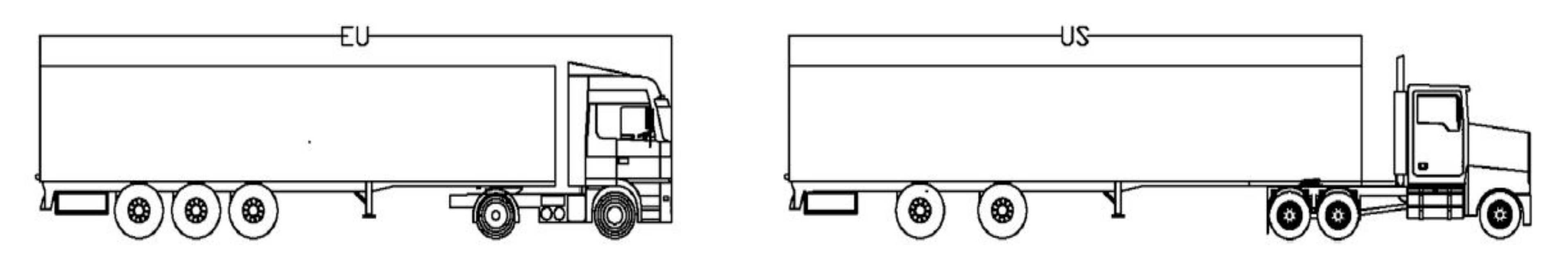
Typically, heavy trucks consist of two simple box-shaped bodies (tractor and trailer) in a tandem arrangement, as shown in Figure 1, and the shape and size of heavy trucks are strongly constrained by practical needs and regulations. As a result, the aerodynamic efficiency of trucks is very low, and a truck requires an estimated 50% of its engine power to overcome its aerodynamic drag at a typical highway cruising speed of 90–100 km/h [2]. At 80 km/h, an approximately 20% reduction in drag can lead to a 10% reduction in fuel consumption, and greater reduction can be achieved at higher speeds, with approximately 15% less fuel consumption at 120 km/h. In Europe, the maximum allowable length includes the whole truck, which ultimately influences the shape of the tractor and therefore the aerodynamic performance of the whole truck. In the United States, only the length of the trailer is fixed, which gives slightly more freedom in designing tractors to be more streamlined. Nevertheless, there is not much that can be done to reduce the aerodynamic drag of a truck through the design or redesign of its shape. An alternative way to reduce aerodynamic drag is through flow control and drag reduction devices [3,4].

There are two main types of drag reduction devices: (i) active devices, which require external energy to manipulate or control flow characteristics (for example, by suppressing flow separation) and usually involve a control system, and (ii) passive devices, add-on devices that alter flow fields at no extra energy expenditure. In comparison, it is easier and more cost effective to implement passive devices. One effective yet relatively simply way to reduce the aerodynamic drag of a truck is to deploy passive drag reduction devices at various regions of the truck.

The aerodynamic drag of a truck is generated mainly in the following four regions [5,6,7]:

• The front part of the truck;
• The tractor–trailer gap;
• The underbody of the truck;
• The rear end of the truck.

For the front part of a truck, some of most common drag reduction devices are cab roof fairing and side fairing. For the rear end of a truck, it has been demonstrated that some simple drag reduction devices with a boat-tail configuration can reduce the aerodynamic drag significantly [8,9]. For the underbody of a truck, side skirts are usually used, and a previous study showed that straight- and flap-type side skirts could significantly alter the flow structures under a vehicle model, leading to reductions in the drag coefficient of 3.1% and 6.1%, respectively [10]. The present study focused on passive drag reduction devices deployed around the tractor–trailer gap region of a simplified truck model.

There are three main types of devices used for reducing aerodynamic drag around the tractor–trailer gap region: tractor (cab) roof deflectors, tractor side extenders, and devices in the gap. One relatively simple drag reduction device used in the gap is called a cross-flow vortex trap device (CVTD) and consists of equally spaced vertical slabs mounted on the front face of the trailer [11]. It was suggested in an experimental study [12] that the drag mechanisms were lower average pressure on the trailer’s front face, removal of flow separation on the leeward side of the trailer due to less gap cross flow, and increased pressure on the back of the tractor. The authors of [12] investigated the effect of the size (horizontal length) of CVTDs on drag reduction, and their results showed that larger CVTDs led to greater drag reduction. It was also found in the same study [12] that the drag reduction performance did not change with the number of CVTDs when that number was between one and four. However, it was demonstrated in a numerical study [13] that while roughly the same drag reduction was obtained using one and two CVTDs, further drag reduction was achieved when three CVTDs were deployed. So far, there have been very limited studies on this specific topic, so to clarify this point, two test cases, with four and five CVTDs, were investigated in the present study. Furthermore, a combination of drag reduction devices could lead to further reductions in aerodynamic drag, as shown in our previous study [14] (three cases: baseline case with cab roof deflector; baseline case with cab roof deflector and side extenders; and baseline case with cab roof deflector, side extenders, and three CVTDs), so this paper presents a further study using a combination of four or five CVTDs, cab roof deflectors, and side extenders.

The numerical method used in the present study was the RANS approach. The computational cost of one other approach, direct numerical simulation (DNS), is hugely expensive, as all details of a turbulent flow are computed directly using a very fine mesh and a very small time step. Hence it is not feasible currently or in the near future to apply DNS for practical engineering flows. Another approach, large-eddy simulation (LES), in which only large scale turbulent motions are computed directly while small scale motions are modeled, is less expensive than DNS and has become more widely used [15,16,17]. However, LES is still very expensive computationally, especially for engineering design simulations and optimization studies where numerous computations need to be performed. Hence, RANS is the most cost-effective yet reasonably accurate approach for practical engineering flow simulations and optimization studies. It has been applied successfully in previous studies similar to the present study [8,13,14,18,19].

This paper is structured as follows: the governing equations and computational details are discussed briefly in Section 2, numerical results and analysis are presented in Section 3, and the concluding remarks are presented in Section 4.

2. Governing Equations and Computational Details

2.1. Governing Equations

The RANS equations are obtained by time averaging the instantaneous three-dimensional governing equations (Navier–Stokes equations) for fluid flows, which are based on the mass and momentum conservation principles. The variables (velocity, pressure) obtained from the RANS approach are hence time-averaged values, usually called mean values. Extra terms, called Reynolds stresses, appear in the RANS equations because of the averaging process, and those terms need to be modeled (approximated) by a turbulence model. Otherwise, the number of unknowns in the RANS equations would be larger than the number of equations. The advantages of the RANS approach are that it is very computationally efficient compared with DNS and LES and that it has been proven to be reasonably accurate for many practical engineering calculations. The main disadvantage of the RANS approach is that only time-averaged variables can be obtained, and hence, instantaneous flow features cannot be captured. Furthermore, in certain flow cases, the results predicted by this approach may not be sufficiently accurate.

In the present study, there was no heat transfer involved, and the velocity was quite low, so the flow was treated as isothermal and incompressible. The RANS equations can be found in many textbooks and publications [20,21,22], so they are presented below very briefly.

Continuity equation:

$$\frac{\partial {\overline{U}}_i}{\partial x_i}=0$$

(1)

Momentum equations:

$$\frac{\partial {\overline{U}}_i{\overline{U}}_j}{\partial x_i}=-\frac{1}{\rho }\frac{\partial \overline{P}}{\partial x_i}+\frac{\partial }{\partial x_i}\left[v\frac{\partial {\overline{U}}_j}{\partial x_i}\right]-\frac{\partial \overline{(u_i^{\prime }{u}_j^{\prime })}}{\partial x_i}$$

(2)

In the above equations ${\overline{U}}_i$ is the mean velocity component in the x, y, and z directions; $\overline{P}$ is the mean pressure; ρ is density; and v is kinematic viscosity. The last term on the right hand of Equation (2) is the Reynolds stress term, and a turbulence model is needed to approximate this term. There are many available turbulence models, but selecting an appropriate one is quite hard, as the performance of these models is usually flow dependent. It was demonstrated in our previous study [14] that among the three highly rated turbulence models tested (the realizable k-ε, the SST k-ω, and a Reynolds stress model), the SST k-ω model predicted the closest drag coefficient (0.809) to the measured value (0.77). Since the present study had the same configuration, apart from the tractor height, with the same flow conditions, the SST k-ω model was employed in the present study.

A commercial computational fluid dynamics (CFD) code, STAR CCM+, was used in the present study. A second-order upwind scheme was selected for spatial discretization, and a pressure-based approach, which is best suited for incompressible flow, was employed, as the flow was treated as incompressible in the present study.

2.2. Computational Details

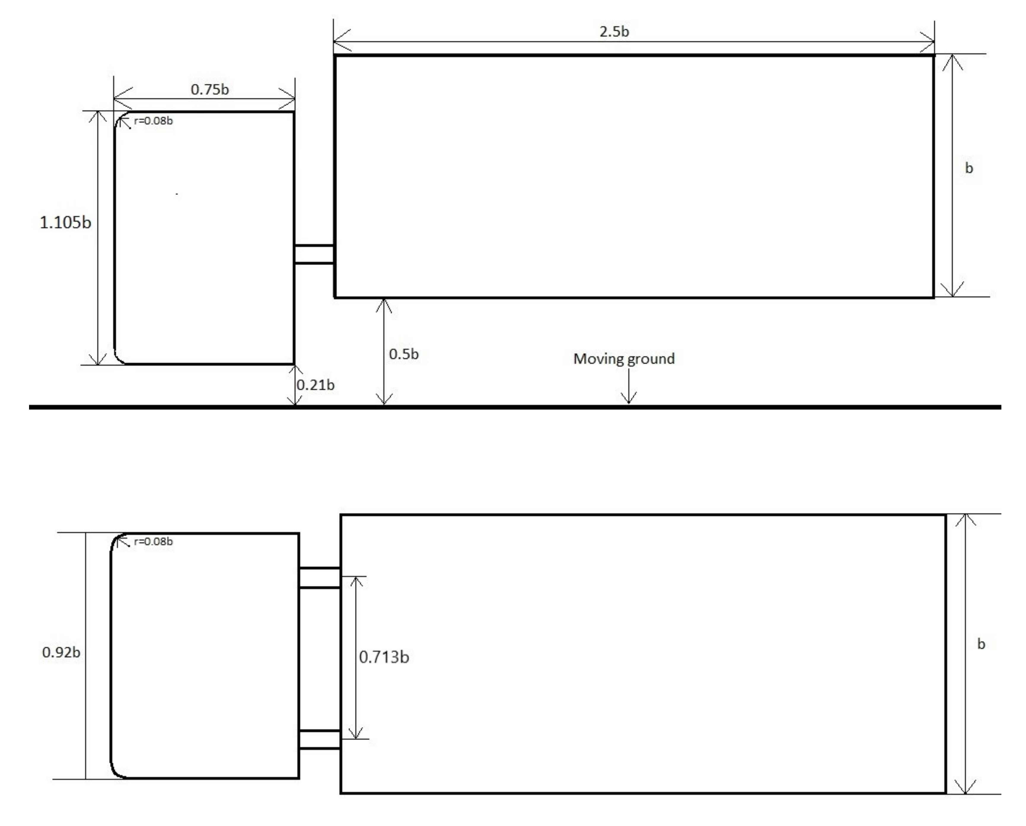
The baseline case in the present study was based on a wind tunnel experiment by Allan [23]. Figure 2 shows a schematic view of the truck model used in the present study, with a Reynolds number of 0.51 × 10⁶ based on the inlet velocity and the height of the trailer. All the dimensions of the truck are shown in Figure 2 as measured relative to the trailer height and width, b = 0.305 m. The gap ratio g/b was equal to 0.17, and the front edges of the tractor were curved at a radius of 0.08b.

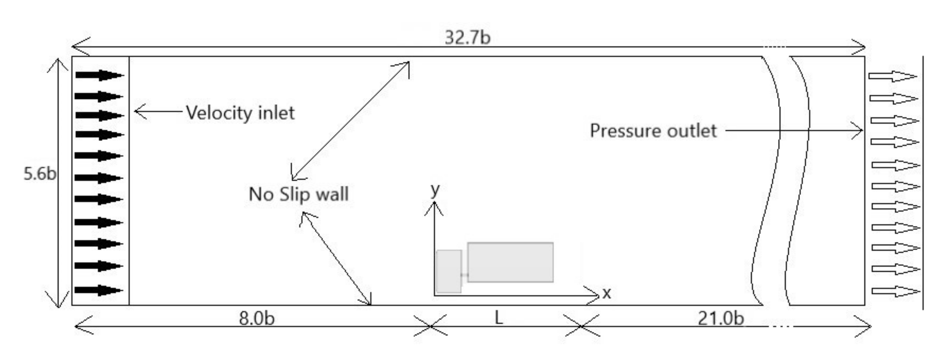
The dimensions of computational domain in the present study were selected to match those of the wind tunnel used in [23]. Figure 3 below shows the side view of the computational domain, with all the dimensions marked on the figure and the width of the domain being 16b.

At the inflow boundary, a constant velocity of 24.4 m/s was specified, matching the value used in [23], and at the outlet, a pressure outlet boundary condition was applied. On the top and side walls, a viscous no-slip wall boundary condition was used, which was also applied to all solid surfaces of the model. To simulate the moving ground condition in the experiment, the streamwise velocity in the horizontal direction was set equal to the inlet velocity on the lower wall, while the vertical velocity was zero. The inlet turbulence intensity was not available from [23], and hence, a representative low-turbulence wind tunnel value of 0.1% was used in the present study.

2.3. Grid Indepedence Study

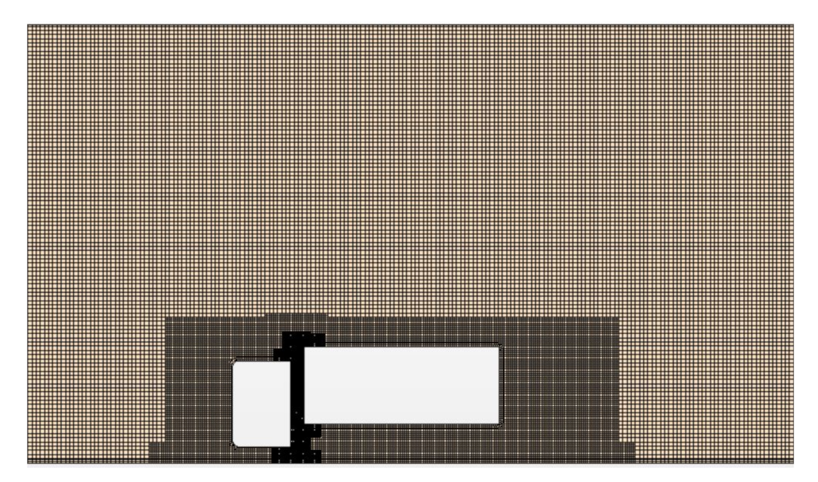
In CFD studies, it is crucial to carry out a grid independence study in order to minimize numerical errors and reduce unnecessary computational cost. Details of the grid independence study can be found in our previous study [14], since the computational domain in the present study was the same as that in [14], and hence the analysis is not repeated here. Figure 4 shows part of the domain and the final mesh of about 5.8 million cells around the truck, with the nearest wall y+ being around 1 so that a wall function was not needed. Figure 4 shows that the mesh was refined in important flow regions around the truck in order to capture accurately the complicated turbulent flow field due to flow separation and recirculation in those regions.

2.4. Test Cases

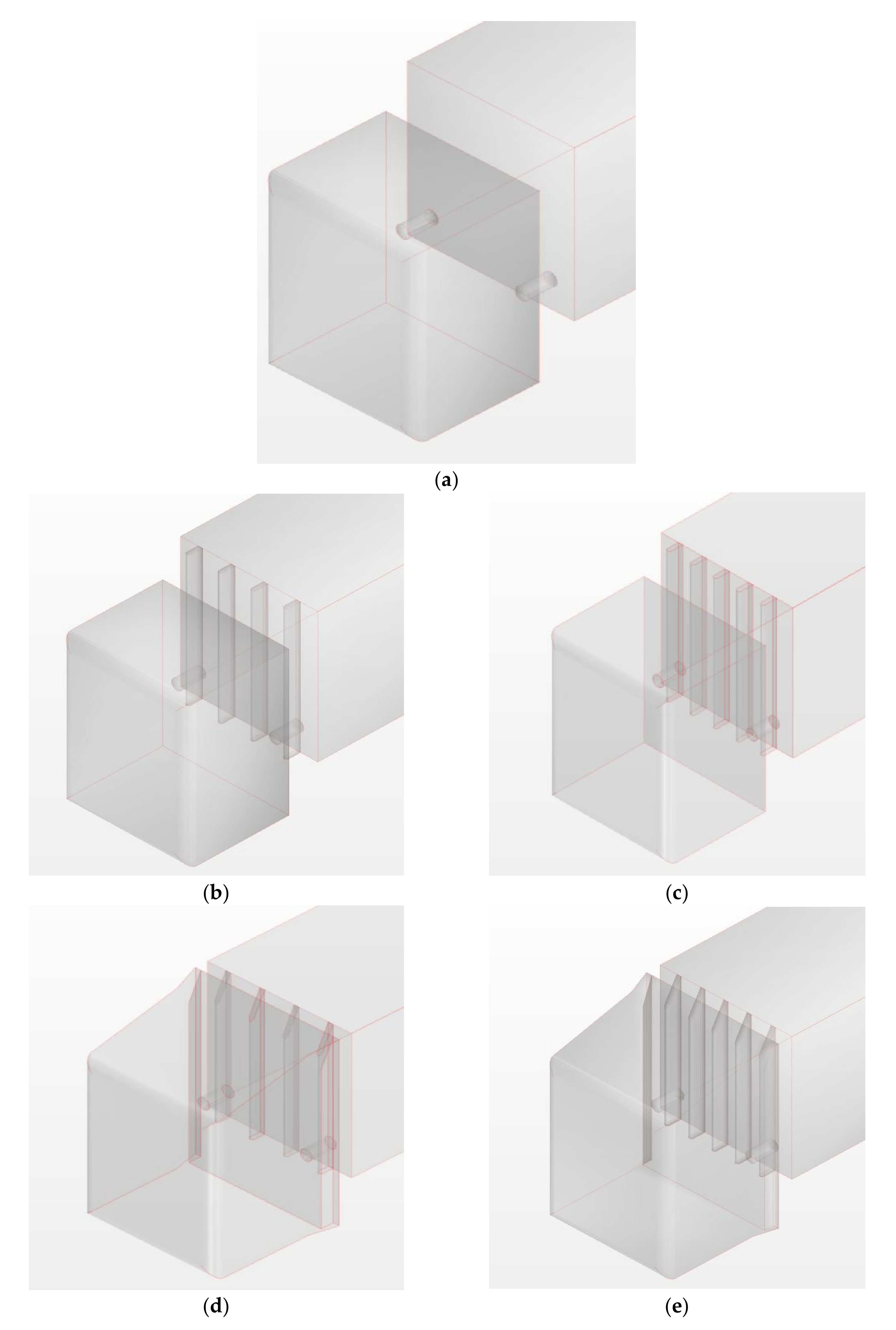
The baseline case and four cases with different configurations of drag reduction devices, as shown in Figure 5, were simulated in the present study.

Baseline case.

• Case 1—baseline case with four CVTDs mounted on the trailer’s front face.
• Case 2—baseline case with five CVTDs mounted on the trailer’s front face.
• Case 3—similar to case 1, plus roof deflector and side extenders.
• Case 4—similar to case 2, plus roof deflector and side extenders.

The dimensions of the CVTDs were 0.026 m in the streamwise direction (x-axis), 0.305 m in the vertical direction (y-axis), and 0.01 in the spanwise direction (z-axis).

3. Results and Discussion

Validation of predictions against experimental data is a very important step in CFD studies to make sure that a computational model is correct and robust. The computational model employed in the present study has already been validated, and comparisons between the predictions obtained from the model and experimental data can be found in our previous studies [5,13,24] and are therefore not presented here again.

3.1. Drag Coefficient

The simulation was run until the residual was down to about 10⁻⁶ and stayed more or less there after about 1500 iterations, indicating that a fully converged solution was obtained. Figure 6 shows the computed drag coefficient (C_d) variation with the number of iterations for the baseline case. C_d hardly changed, confirming that a fully converged solution was obtained. C_d was obtained as an output parameter from the CFD code (STAR CCM+) used in the present study based on three inputs: a reference area, air density, and inlet velocity.

Table 1. Predicted drag coefficients (C_d) and corresponding drag reduction.

	Cd	Drag Reduction
Baseline	0.537
Case 1	0.522	2.8%
Case 2	0.516	3.9%
Case 3	0.421	21.6%
Case 4	0.407	24.2%

shows the predicted drag coefficients for the baseline case and the four cases with drag reduction devices in the present study. The reference area used for the drag coefficient computation was the trailer front surface area (bxb). The percentage drag reduction presented below was defined as 100 × (C_d-baseline − C_d-cases)/C_d-baseline. It is obvious that drag reductions were obtained for all four cases compared with the baseline case, especially for cases 3 and 4, where significant drag reductions were achieved (21.6% and 24.2%). For case 1, with four CVTDs mounted on the trailer front, 2.8% drag reduction was obtained against the baseline case. When five CVTDs were deployed in case 2, 3.9% drag reduction was obtained against the baseline case, representing 1.1% further drag reduction compared with case 1. This demonstrates that deployment of more CVTDs can lead to slightly more drag reduction. However, the benefits of adding more CVTDs may diminish, and it becomes impracticable to mount more and more CVTDs on the limited area of the trailer’s front face. As demonstrated in our previous study [14], combinations of different drag reduction devices (CVTDs, roof deflector and side extender) represent the most effective way to reduce the aerodynamic drag. This was confirmed in the present study, since 21.6% and 24.2% drag reductions against the baseline case were obtained for cases 3 and 4, respectively, where CVTDs plus a roof deflector and side extenders were deployed. An in-depth flow field analysis is presented below to elucidate how the drag reduction was achieved.

3.2. Surfcae Pressure Distribution

The total drag of a vehicle consists of two parts and is generated by two different mechanisms: skin friction drag due to the friction force between the air and vehicle surface and form drag or pressure drag due to the pressure difference on the front and back areas of the vehicle. In the case of a heavy truck, as in the present study or any bluff body, the total drag is due mainly to pressure drag. Therefore, the analysis in the present study focused on the pressure distribution on the trailer’s front face, as the pressure on the tractor’s front face and the trailer’s back face would remain the same. In other words, the drag reduction device configurations investigated in the present study mainly manipulated the pressure on the trailer’s front face.

Figure 7 shows contours of the pressure coefficients for the baseline and four cases in the present study. As mentioned above, the drag reduction devices deployed in the present study resulted mainly in pressure changes on the trailer’s front face. This is evident from Figure 7, since the pressure distributions on the front face of the tractor are virtually the same for all the cases. However, the pressure distributions in the four cases were different from the baseline case on the trailer’s front face, as can be seen clearly from Figure 7. For the baseline case, there was a high and uniform pressure region on the top part of the trailer’s front surface, as shown in Figure 7a. This was because the tractor top surface was not at the same level with the trailer top surface, so a certain amount of flow directly impinged onto the top part of the trailer’s front surface. For case 1, as shown in Figure 7b, this high-pressure region on the top part of the trailer’s front face was still there, but with slight reductions in both the area and pressure, resulting a drag reduction. For case 2, as shown in Figure 7c, this high-pressure region was slightly further reduced when one more CVTD was employed, especially in a small region of the middle part of the trailer’s front face where the pressure decreased, leading to a further drag reduction for case 2. There was a small, long, narrow region near the edges of the trailer’s front face where the pressure was reasonably high, as shown in Figure 7a for the baseline case. This region was slightly reduced in both cases 1 and 2 as shown in Figure 7b,c, which also contributed to the drag reduction for these cases. However, for cases 3 and 4, those high-pressure regions on the trailer’s front face were eliminated completely, as shown in Figure 7d,e, when the roof deflector and side extenders were deployed, leading to significant drag reductions as shown in Table 1. This was because the deployment of the roof deflector and side extenders prevented the flow impingement onto the trailer’s front face. Further analysis of flow filed is presented below to shed light on how these drag reduction devices changed the flow fields inside the gap.

3.3. Flow Field

Figure 8 presents the predicted velocity vectors on the XZ plane at y = 0.2 m for the baseline and four cases in the present study. The flow fields inside the gap region in all four cases were quite different from those in the baseline case and from each other as a result of the deployment of different drag reduction devices. In the baseline case, three vortices were clearly observable, and there was a relatively strong cross flow within the gap, as shown in Figure 8a. Figure 8b shows that for case 1, with four CVTDs, those three vortices were broken down, and a few recirculation regions were formed locally between each CVTD, leading to a reduction in cross flow. This indicates that the deployment of four CVTDs in case 1 stabilized the flow to some extent compared with the situation in the baseline case. For case 2, with five CVTDs, the flow was further stabilized slightly, or more constrained because of the additional CVTD, leading to a further reduction in cross flow, as shown in Figure 8c. When the roof deflector and side extenders were added in cases 3 and 4, the amount of flow entering the gap region from the top and side was significantly reduced, resulting in a smooth cross-flow field and a significant reduction in cross flow, as shown in Figure 8d,e. This confirms that CVTDs were capable of stabilizing the flow within the gap and hence may result in a reduction in the turbulence level. Nevertheless, the major reason for the smooth cross-flow field within the gap was the reduced flow entering the gap from the top and both sides as a result of deploying the roof deflector and side extenders.

Figure 9 shows the velocity vectors on an YZ plane within the gap region for the baseline and four cases. It can be seen that complicated flow field is formed in the gap for the baseline case with cross flow at the bottom half, especially there are three distinct vortices formed towards the bottom as shown in Figure 9a. The cross flow and those three vortices were eliminated for all four cases when CVTDs were deployed, leading to less turbulent flow. For the baseline case and cases 1 and 2, there was a very strong down flow due to the amount of flow entering from the top of the gap region, as shown in Figure 9a–c. This down flow was reduced significantly by the use of the roof deflector mounted on top of the tractor for cases 3 and 4, as shown in Figure 9d,e. It is obvious that the flow became relatively much smoother with the deployment of drag reduction devices, especially in cases 3 and 4, when the roof deflector, side extenders, and CVTDs were all used. Further analysis of turbulence intensity in the gap is presented below to show how the turbulence level changed when those drag reduction devices were used.

3.4. Turbulence Intensity

To clarify the point at which the flow became less turbulent, Figure 10 presents the turbulence intensity for the baseline and four cases on the YZ plane at x = 0.26 m inside the gap. Only the lower part of the region, with a relatively high turbulence level, is shown in Figure 10, since turbulence level was very low and hardly visible on the top part of the region. For the baseline case, there were a few regions where the turbulence intensity was above 4%, with the maximum value being about 6%, as shown in Figure 10a. For cases 1 and 2, the turbulence intensity was indeed reduced, with the maximum value being below 4%, as shown in Figure 10b,c. However, interestingly, the turbulent flow region increased compared with the baseline case, especially in case 2, when five CVTDs were employed. As shown in Figure 10d,e, in cases 3 and 4, there were significant reductions in turbulence intensity, and the flow actually became more or less laminar in most regions, apart from the bottom part, where the maximum turbulence intensity was about 3%. This was due to much less flow entering the gap when the roof deflector and side extenders were used and especially to the much reduced interactions between flow entering from top of the gap and flow entering from sides of the gap. The stabilizing flow with less turbulent kinetic energy may be beneficial, as less kinetic energy would be lost (dissipated), which could possibly lead to less drag, as in the case of an aircraft wing, where induced drag can be reduced by the use of a winglet to diminish the kinetic energy loss of the wing-tip vortices. However, it is worth pointing out that a major part of the drag reduction was due to the deployment of the roof deflector, which prevented the flow impingement directly onto the top part of the trailer’s front face, resulting in the elimination of the high-pressure region on the top part of the trailer’s front face, and the side extenders, which further eliminated the small, long, narrow high-pressure regions near the edges of the trailer’s front face.

4. Conclusions

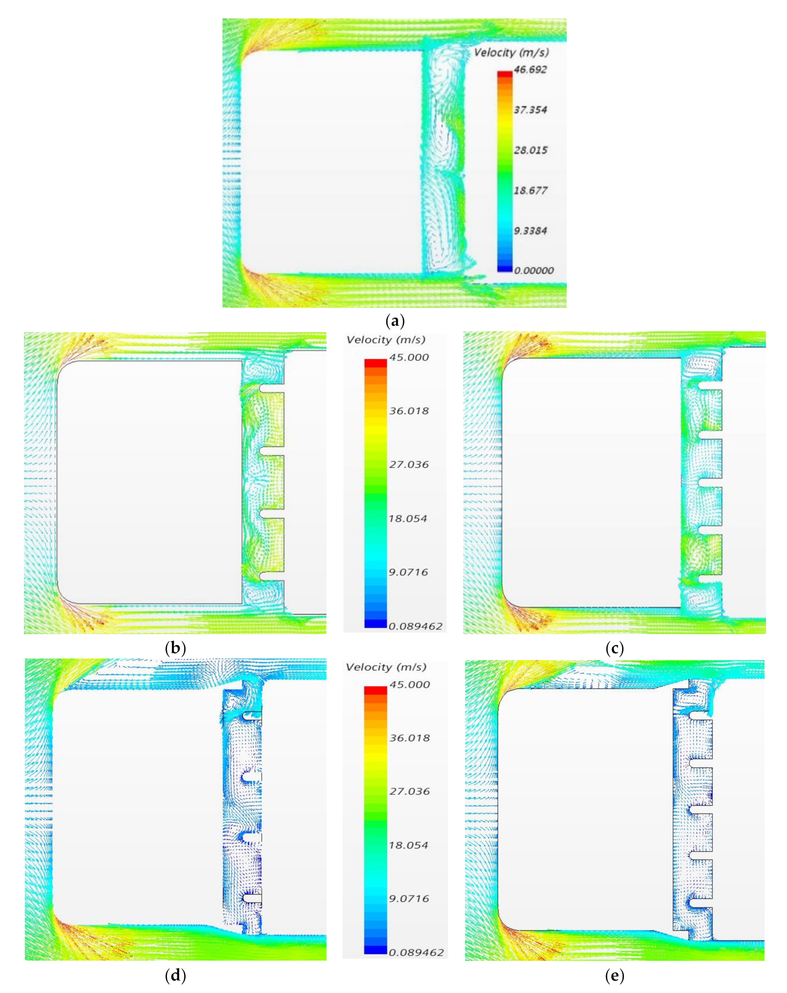
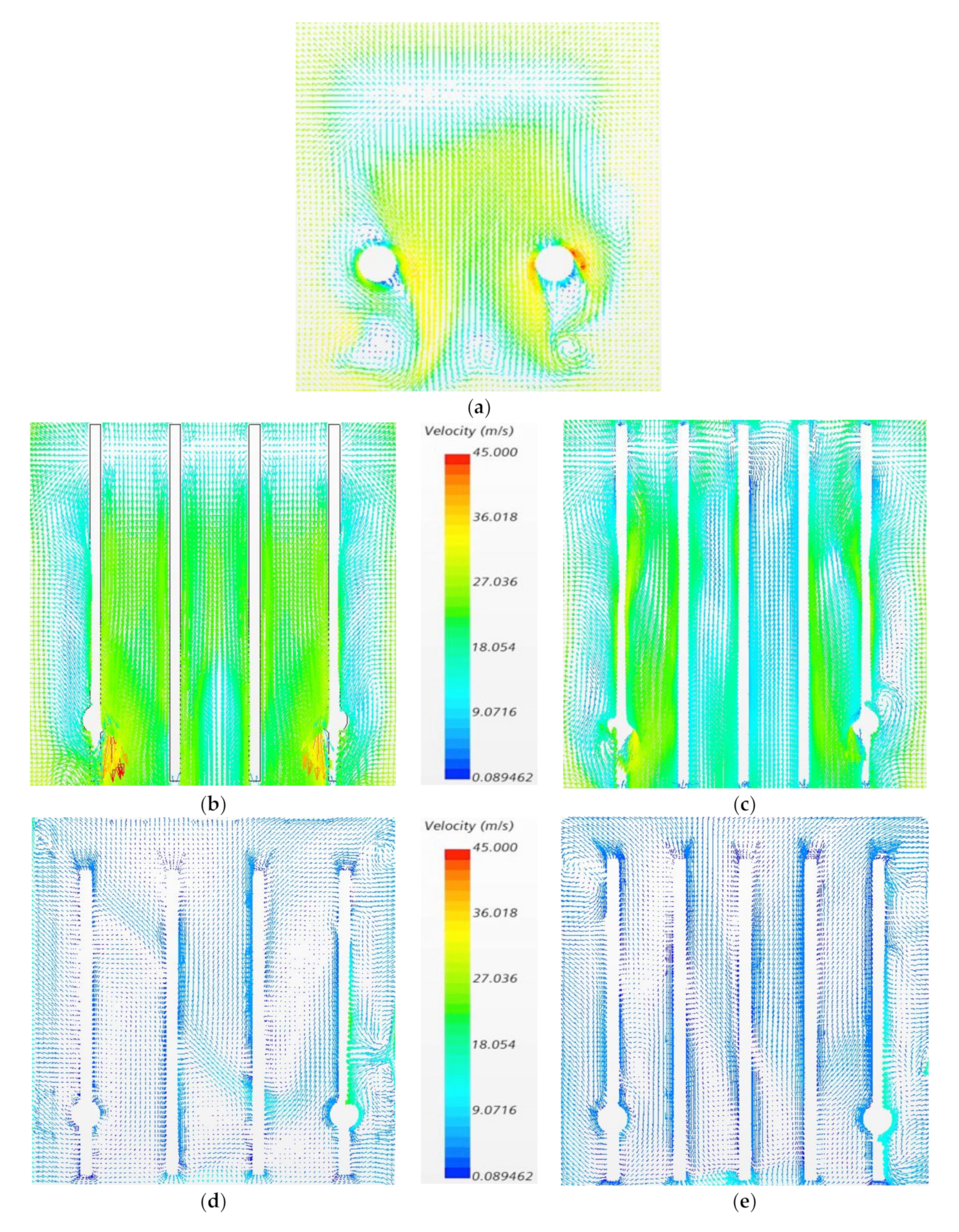
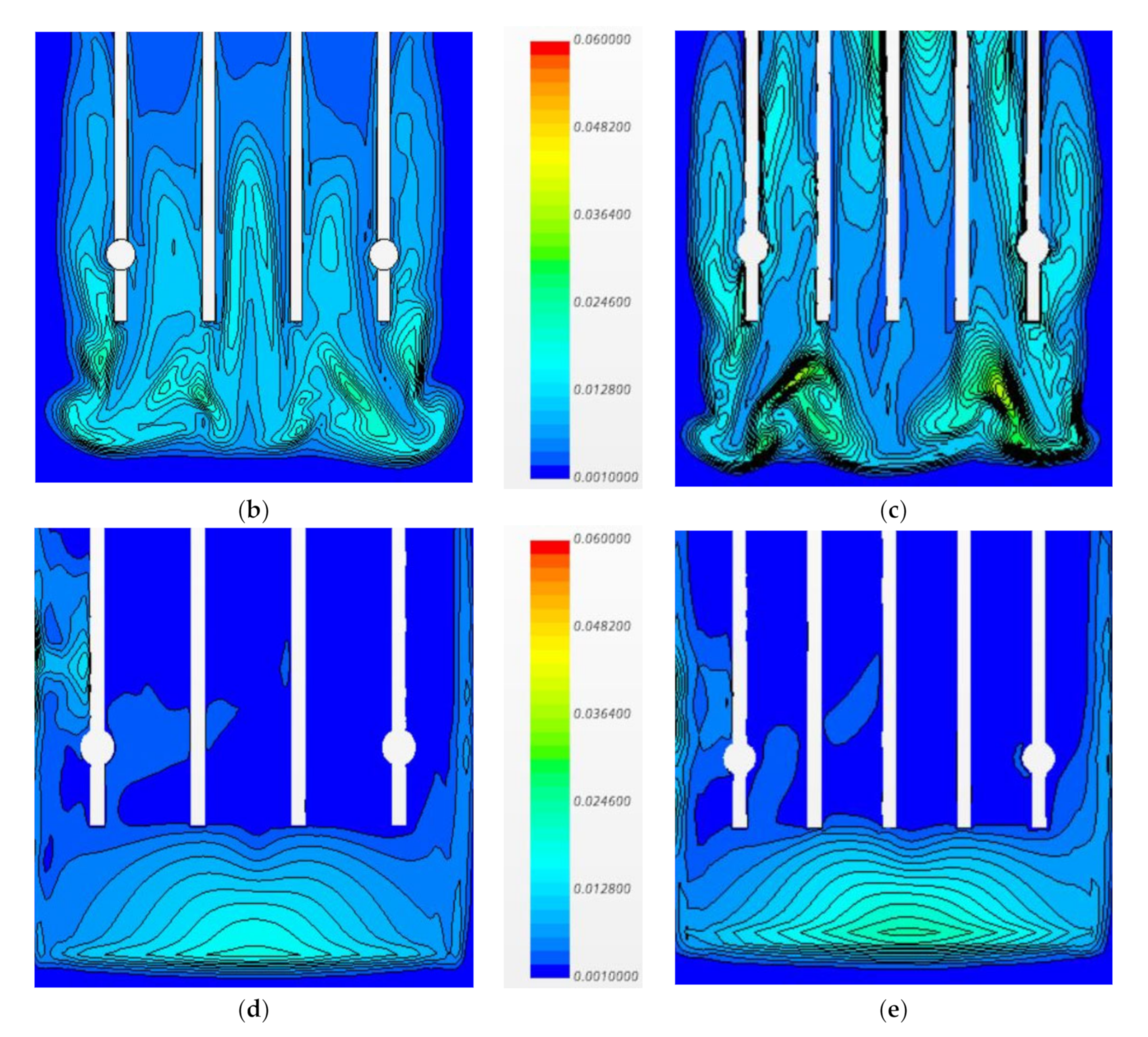
Turbulent flow over a simplified tractor–trailer truck model was simulated using the RANS approach to assess the effectiveness of four drag reduction device configurations deployed on the tractor and gap region. The surface pressure distributions, velocity fields, and turbulence intensity levels in the gap region were thoroughly analyzed to understand how the drag reduction was achieved for those four configurations. The main findings are summarized as follows:

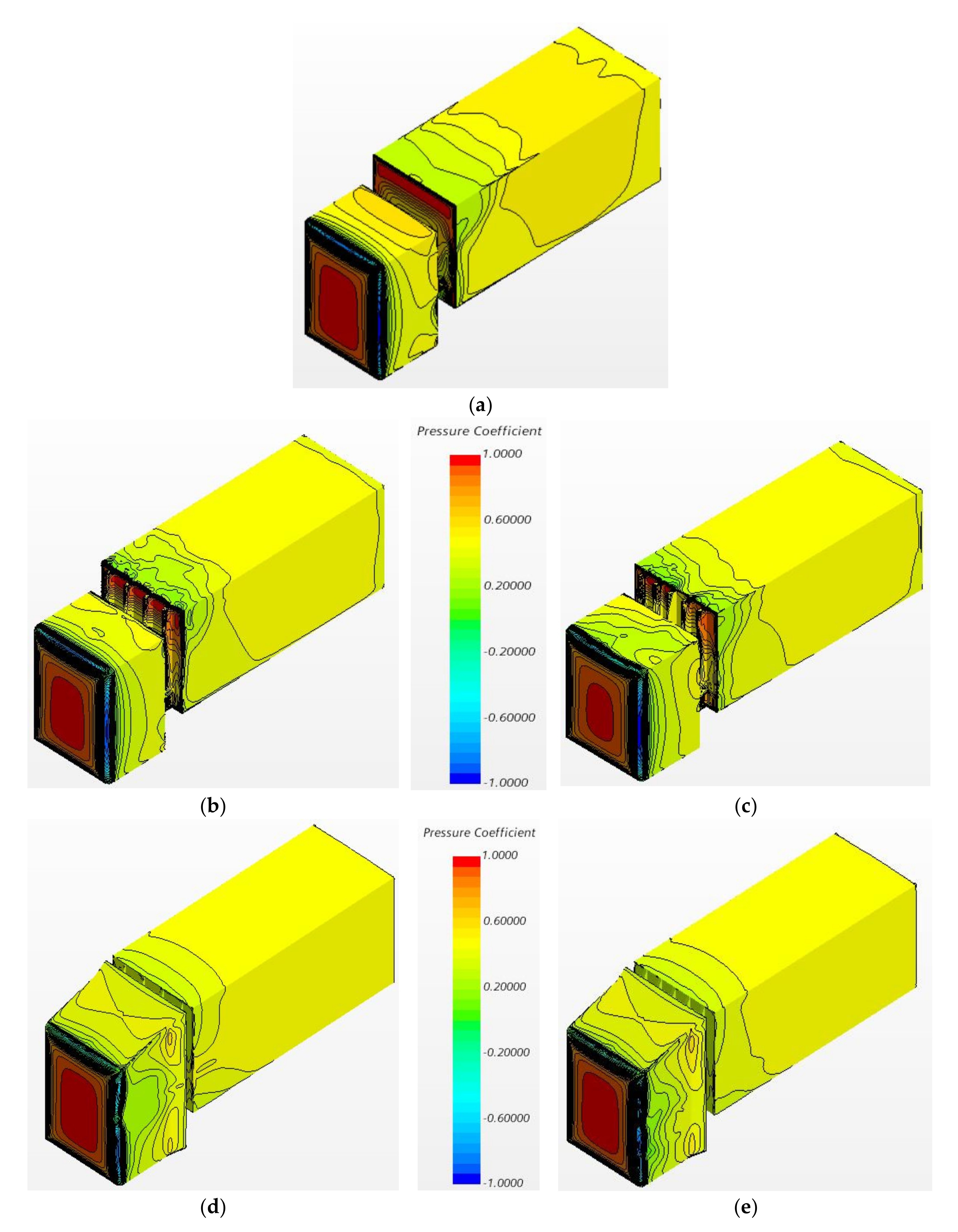
This study further confirmed that the major drag reduction mechanism was the elimination of a high-pressure region on the top part of the front face of the trailer, whereas the reduction in the turbulence level by stabilizing the flow inside the gap region via the use of CVTDs played only a minor role in the overall drag reduction.

The most effective drag reduction configuration among the four different configurations tested in the current study was case 4, with a roof deflector, side extenders, and five CVTDs. The employment of the roof deflector on top of the tractor successfully eliminated the high-pressure region on the top part of the front face of the trailer more or less completely, making it the main contributor to the overall drag reduction. In addition, it cut down the amount of flow entering the gap region significantly, which helped to reduce the turbulence level inside the gap region.

The use of side extenders resulted in the elimination of two narrow, vertical high-pressure regions near the edges of the trailer’s front face, which contributed to a further drag reduction. These two narrow, vertical high-pressure regions were formed because the width of the tractor was slightly smaller than that of the trailer, so a small amount of flow impinged directly onto those two regions. The use of side extenders prevented this flow impingement and hence eliminated those two high-pressure regions. Furthermore, the amount of flow entering the gap region from both sides was reduced by the side extenders, which helped to reduce the interaction of flow inside the gap region, leading to an additional reduction in the turbulence level.

The CVTDs mounted on the front face of the trailer had several benefits: 1. reduction in the inward turning flow from both sides of the gap; 2. stabilization of the flow inside the gap region; 3. decreased cross flow inside the gap region. Nevertheless, the amount of drag reduction due to the use of CVTDs themselves was limited, and slightly more drag reduction is achieved with five CVTDs than four.

References

1. Bearman, P. Bluff body flow research with application to road vehicles. In The Aerodynamics of Heavy Vehicles II: Trucks, Buses and Trains; Browand, F., McCallen, R., Ross, J., Eds.; Springer: Berlin, Germany, 2009; Volume 41, pp. 3–13. [Google Scholar]
2. Schoon, R. On-road evaluation of devices to reduce heavy truck aerodynamic drag. In Proceedings of the SAE 2007 Commercial Vehicle Engineering Congress & Exhibition, Rosemont, IL, USA, 30 October–1 November 2007; Available online: https://saemobilus.sae.org/content/2007-01-4294/ (accessed on 18 May 2022).
3. Choi, H.; Lee, J.; Park, H. Aerodynamics of Heavy Vehicles. Annu. Rev. Fluid Mech. 2014, 46, 441–468. [Google Scholar] [CrossRef]
4. Minelli, G.; Hartono, E.; Chernoray, V.; Hjelm, L.; Basara, B.; Krajnovic, S. Development of active flow control for trucks. In Proceedings of the 3rd Thermal and Fluids Engineering Conference (TFEC), Fort Lauderdale, FL, USA, 4–7 March 2018. [Google Scholar]
5. Charles, T.; Lu, Y.; Yang, Z. Impacts of the gap size between two bluff bodies on the flow field within the gap. In Proceedings of the 13th International Conference in Heat Transfer, Fluid Mechanics and Thermodynamics, Portorož, Slovenia, 17–19 July 2017. [Google Scholar]
6. Castejon, L.; Mirables, R. Aerodynamic Analysis of Some Boat Tails for Heavy Vehicles. Int. J. Heavy Veh. Syst. 2012, 19, 115–127. [Google Scholar]
7. Wood, R. A discussion of a heavy truck advanced aerodynamic trailer system. In Proceedings of the 9th International Symposium on Heavy Vehicle Weights and Dimensions, State College, PA, USA, 18–22 June 2006. [Google Scholar]
8. Abikan, A.; Yang, Z.; Lu, Y. Computational Analysis of Turbulent Flow over a Bluff Body with Drag Reduction Devices. J. Appl. Comput. Mech. 2020, 6, 1210–1219. [Google Scholar]
9. Khalighi, B.; Balkanyi, S.R.; Bernal, L.P. Experimental Investigation of Aerodynamic Flow over a Bluff Body in Ground Proximity with Drag Reduction Devices. Int. J. Aerodyn. 2013, 3, 217–233. [Google Scholar] [CrossRef]
10. Kim, J.J.; Lee, S.J. Drag-reducing underbody flow of a heavy vehicle with side skirts. J. Vis. 2017, 20, 369–378. [Google Scholar] [CrossRef]
11. Bauer, S.; Wood, R. Simple and Low Cost Aerodynamic Drag Reduction Devices for Tractor Trailer Trucks. SAE Technical Paper. 2003. Available online: https://saemobilus.sae.org/content/2003-01-3377/ (accessed on 18 May 2022).
12. Story, J.; Garcia, I.; Babinsky, H. The Effect of Cross-Flow Vortex Trap Devices on the Aerodynamic Drag of Road Haulage Vehicles. SAE Technical Paper. 2021. Available online: https://saemobilus.sae.org/content/2021-01-5040/ (accessed on 18 May 2022).
13. Charles, T.; Yang, Z.; Lu, Y. Numerical Analysis of Flow in the Gap between a Simplified Tractor-Trailer Model with Cross Vortex Trap Device. Int. J. Mech. Mechatron. Eng. 2019, 13, 707–711. [Google Scholar]
14. Charles, T.; Yang, Z.; Lu, Y. Assessment of Drag Reduction Devices Mounted on a Simplified Tractor-Trailer Truck Model. J. Appl. Comput. Mech. 2021, 7, 45–53. [Google Scholar]
15. Yang, Z. Large-eddy simulation: A glance at the past, a gaze at the present and a glimpse at the future. In Proceedings of the 5th International Symposium on Jet Propulsion and Power Engineering, Beijing, China, 15–19 September 2014. [Google Scholar]
16. Yang, Z. High fidelity numerical simulations of gas turbine flows. In Proceedings of the 3rd Chinese International Turbomachinery Conference (CITC), Chongqing, China, 12–14 April 2018. [Google Scholar]
17. Bennett, W.; Yang, Z.; McGuirk, J.J. Large-eddy simulation of effusion cooling flows. In Proceedings of the 2nd International Symposium on Jet Propulsion and Power Engineering, Guilin, China, 22–26 September 2008. [Google Scholar]
18. Charles, T.; Yang, Z.; Lu, Y. Computational Study of Flow around 2D and 3D Tandem Bluff Bodies. J. Appl. Comput. Mech. 2021, 7, 528–534. [Google Scholar]
19. Kumar, P.; Chaurasia, N. Enhancement of Aerodynamic Efficiency of Truck-Trailer. Int. J. Innov. Res. Sci. Eng. Technol. 2016, 5, 9563–9573. [Google Scholar]
20. Zikanov, O. Essential Computational Fluid Dynamics, 2nd ed.; John Wiley & Sons: Hoboken, NJ, USA, 2019. [Google Scholar]
21. Worth, N.; Yang, Z. Simulation of an Impinging Jet in a Crossflow Using a Reynolds Stress Transport Model. Int. J. Numer. Methods Fluids 2006, 52, 199–211. [Google Scholar] [CrossRef]
22. Yang, Z. Assessment of Unsteady-RANS Approach against Steady-RANS Approach for Predicting Twin Impinging Jets in a Cross-Flow. Cogent Eng. 2014, 1, 936995. [Google Scholar] [CrossRef] [Green Version]
23. Allan, J. Aerodynamic drag and pressure measurements on a simplified tractor-trailer model. J. Wind Eng. Ind. Aerodyn. 1981, 9, 125–136. [Google Scholar] [CrossRef]
24. Charles, T. Numerical Study of Tractor-Trailer Gap Aerodynamics. Ph.D. Thesis, University of Derby, Derby, UK, December 2020. [Google Scholar]
Figure 1. A schematic view of European and American heavy trucks.
Modelling 03 00019 g001
Figure 2. Schematics of the tractor–trailer truck model.
Modelling 03 00019 g002
Figure 3. Computational domain.
Modelling 03 00019 g003
Figure 4. Side view of the mesh around the truck.
Modelling 03 00019 g004
Figure 5. Baseline and four cases with different configurations of drag reduction devices: (a) baseline case; (b) Case 1; (c) Case 2; (d) Case 3; (e) Case 4.
Modelling 03 00019 g005
Figure 6. The predicted Cd variation with the number of iterations.
Modelling 03 00019 g006
Figure 7. Contours of surface pressure coefficient: (a) baseline case; (b) Case 1; (c) Case 2; (d) Case 3; (e) Case 4.
Modelling 03 00019 g007
Figure 8. Velocity vectors on the XZ plane at y = 0.2 m: (a) baseline case; (b) Case 1; (c) Case 2; (d) Case 3; (e) Case 4.
Modelling 03 00019 g008
Figure 9. Velocity vectors on the YZ plane in the gap at x = 0.26 m: (a) baseline case; (b) Case 1; (c) Case 2; (d) Case 3; (e) Case 4.
Modelling 03 00019 g009
Figure 10. Turbulence intensity on the YZ plane at x = 0.026 m: (a) baseline case; (b) Case 1; (c) Case 2; (d) Case 3; (e) Case 4.
Modelling 03 00019 g010aModelling 03 00019 g010b