1. Introduction
A three-dimensional (3D) model of factory buildings and inventory, as well as the simulation of process steps, play a major role in different planning domains. In general, virtual planning has many advantages when compared to analogue planning. The most stringent benefit is the detection of planning mistakes early on in the planning process. This is favourable, as planning mistakes are detected well before implementation [
1], i.e., before factory ramp-up, before new machinery is ordered, before construction is under way, or before the production process is detailed. This is due to the fact that the structure and layout of the building influence several other domains. A changing building model can entail changes in spatial availability for production or logistics assets. Thus, the layout of production lines or the concept of machines may have to be adapted accordingly. Further, virtual planning reduces travel efforts, as planners do not have to meet on-site to discuss modifications or reorganizations. They can rather meet in a multi-user simulation model or a virtual reality supported 3D environment, which saves a substantial amount of travel time and cost. Digital 3D models are the basis for building reorganizations as well as the introduction of completely new or modified manufacturing process steps.
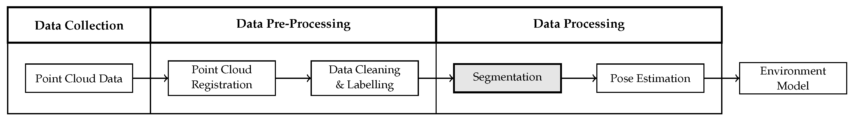
There are several challenges to tackle in order to determine the as-is state of a production plant. First of all, the current data in the respective plant have to be collected. In order to acquire 3D information, laser scanning and photogrammetry are useful digitalization techniques. After plant digitalization, the collected data have to be pre-processed, including data fusion of inputs from different sources, as well as subsequent data cleaning and labelling. The data fusion includes a registration step, where the point clouds from different scans or different sources are fused in a common global coordinate system. However, simulating the factory or the assembly process on the basis of the pre-processed point clouds alone is not possible. Generally, the point clouds generated by laser scanners and photogrammetry techniques suffer from occlusions, i.e., a set of objects blocks the sight to other objects, which results in holes within the point cloud. For instance, the outcomes of collision checking are not reliable when the point cloud is not complete. Additionally, a point cloud does not contain any information regarding how to separate different objects. Therefore, the introduction of new or the displacement of existing objects is time consuming, as the respective set of points has to be selected manually. A segmentation step can be introduced in order to separate different objects from one another automatically. Finally, to generate an environment model, the poses of the relevant objects need to be estimated and the point sets have to be replaced by computer-aided design (CAD) models.
Figure 1 summarizes the process for generating an environment model on the basis of a point cloud, which was introduced in our previous work [
2]. Each of the process steps can be subdivided into further building blocks. This paper discusses the segmentation step in more detail. The remaining process steps are described in our next contribution.
The semantic segmentation of a point cloud is widely solved using deep neural networks. Most of the existing deep learning architectures make use of the frequentist notion of probability. However, these so-called frequentist neural networks suffer from two major drawbacks. They do not quantify uncertainty in their predictions. Often, the softmax output of frequentist neural networks is interpreted as network uncertainty, which is, however, not a good measure. The softmax function only normalizes an input vector but cannot as such be interpreted as network (un)certainty [
3]. Especially for out of distribution samples, the softmax output can give rise to misleading interpretations [
4]. In the case of deep learning frameworks being integrated into safety critical applications, like autonomous driving, it is important to know what the network is uncertain about. There was one infamous accident that was caused by a partly autonomous driving car that confused the white trailer of a lorry with the sunlit sky or a bright overhead sign [
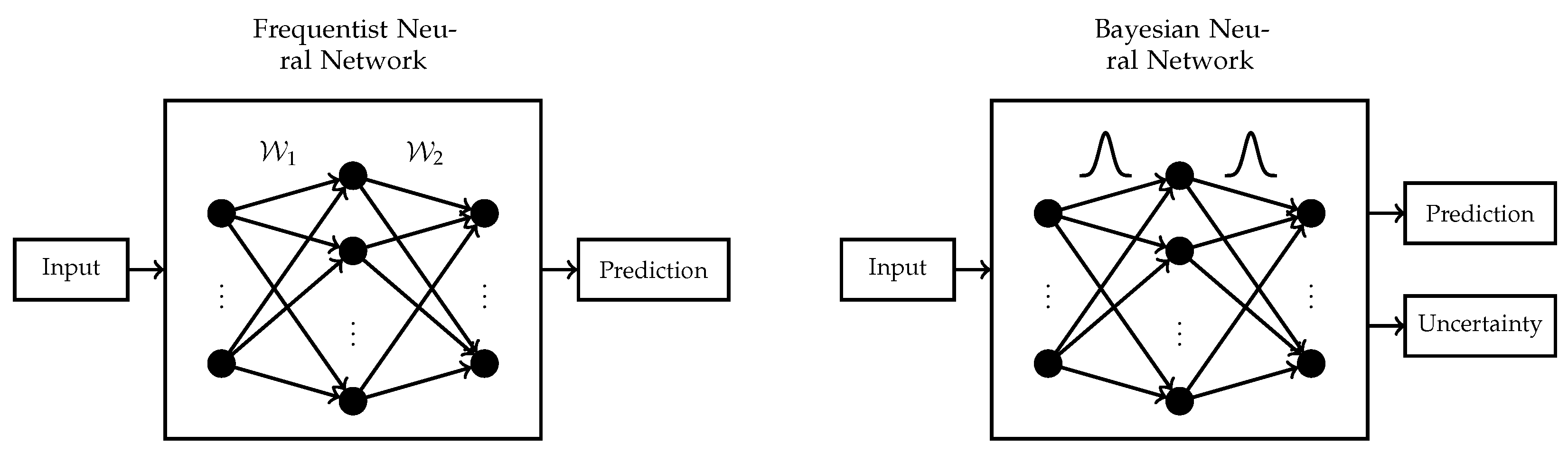
5]. By considering network uncertainties, similar scenarios could be mitigated. In frequentist neural networks, the network parameters
are point estimates, whereas, in Bayesian neural networks, a distribution is placed over all the network parameters. Conceptually, the network optimization is more complex for Bayesian neural networks; however, they allow for additional quantification of network uncertainty.
Figure 2 summarizes the differences between a single hidden layer frequentist and Bayesian neural network. Another shortcoming of frequentist neural networks is their tendency to overfit on small data sets with a high number of features. However, in this work, we focus on uncertainty estimation rather than the challenge of feature selection.
We present a novel Bayesian 3D point cloud segmentation framework that is based on PointNet [
6], which is able to capture uncertainty in network predictions. The network is trained using variational inference with multivariate Gaussians with a diagonal covariance matrix as variational distribution. This approach hardly adds any additional parameters to be optimized during each backward pass [
7]. Further, we formulate an approximate Bayesian neural network by applying dropout training, as suggested in [
3]. We use an entropy based interpretation of uncertainty in the network outputs and distinguish between overall, data related, and model related uncertainty. These types of uncertainty are called predictive, aleatoric, and epistemic uncertainty, respectively [
8]. It makes sense to consider this differentiation, as it shows which predictions are uncertain and to what extent this uncertainty can be reduced by further model refinement. The remaining uncertainty after model optimization and training is then inherent to the underlying data set. Other notions of uncertainty that are based on the variance or credible intervals of the predictive network outputs are discussed and evaluated. To the best of our knowledge, no other work has treated the topic of uncertainty estimation and Bayesian training of 3D segmentation networks that operate on raw and unordered point clouds without a previous transformation into a regular format. We embed all of the proposed networks in an industrial prototype for environment modelling in an automotive assembly plant. Aside from an automotive data set that is collected by the authors at a German manufacturing plant, the proposed networks are evaluated on a scientific data set in order to ensure the comparability with other state-of-the-art frameworks. Summing up, the contributions of this paper are:
Workflow: we describe how to quantify uncertainty in segmentation frameworks that operate on raw and unstructured point clouds. Further, it is discussed how to use this information for improving the generation of factory models.
Framework: we formulate a 3D segmentation model that is trained in a fully Bayesian way using variational inference and an approximate Bayesian model, which is derived by the application of dropout training.
Experiment: we evaluate how the different sources of uncertainty affect the neural networks’ segmentation performance in terms of accuracy. Further, we outline how the factory model can be improved by considering uncertainty information.
The remainder of this paper is organized in the following way.
Section 2 conducts a thorough literature review on 3D point cloud processing frameworks, including deep neural networks, Bayesian neural networks, and uncertainty quantification. In the subsequent
Section 3, the frequentist, the approximate Bayesian, and the fully Bayesian models are described in more detail.
Section 4 discusses the scientific and industrial data sets that are used for the evaluation of our models and elaborates their characteristics. The models are evaluated with respect to their performance in
Section 5. Finally,
Section 6 provides a discussion, which describes the bigger scope of this work and concludes the paper.
2. Literature Review
The following paragraphs cast light upon prior research in the areas of 3D point cloud processing as well as Bayesian neural networks and uncertainty estimation. The neural networks that are discussed in the first section are all based on the classical or frequentist interpretation of probability. Bayesian neural networks, rather, take on the Bayesian interpretation of probability, which views probability as a personal degree of belief.
2.1. 3D Point Cloud Processing
In contrast to images that have a regular pixel structure, point clouds are irregular and unordered. Further, they do not have a homogeneous point density, due to occlusions and reflections. Neural networks that process 3D point clouds have to tackle all of these challenges. Most of the networks are based on the frequentist interpretation of probability and they are divided into three classes based on the format of their input data. There are deep learning frameworks that consume voxelized point clouds [
9,
10,
11,
12], collections of two-dimensional (2D) images that are derived by transforming 3D point clouds to the 2D space from different views [
8,
13,
14], and raw unordered point clouds [
6,
15,
16]. On the one hand, the voxelization of point clouds has the advantage of providing a regular structure apt for the application of 3D convolutions. On the other hand, it renders the data unnecessarily big, as unoccupied areas of the point cloud are still represented by voxels. Generally, this format conversion introduces truncation errors [
6]. Further, voxelization reduces the resolution of the point cloud in dense areas, which leads to a loss of information [
17]. Transforming 3D point clouds to 2D images from different views allows for the application of standard 2D convolutions having the advantage of elaborate kernel optimizations. Yet, the transformation to a lower space can cause the loss of structural information embedded in the higher dimensional space. Additionally, in complex scenes, a high number of viewports have to be taken into account in order to describe the details of the environment [
17]. For this reason, the following work focuses on the segmentation of raw point clouds.
In order to generate a factory model out of raw point clouds, the objects of interest have to be detected and their pose needs to be estimated. One approach that extracts six degrees-of-freedom (DoF) object poses, i.e., the translation and orientation with respect to a predefined zero point, in order to generate a simulation scene is presented in [
18]. The framework is called Scan2CAD, and it describes a frequentist deep neural network that consumes voxelized point clouds as well as CAD models of eight household objects and directly learns the 6DoF CAD model alignment within the point cloud. The system that is presented in [
19] has similar input data and estimates the 9DoF pose, i.e., translation, rotation and scale, of the same household objects. A framework for the alignment of CAD models, which is based on global descriptors computed by using the Viewpoint Feature Histogram approach [
20] rather than neural networks, is discussed in [
21]. Generally, direct 6DoF or 9DoF pose estimation on the basis of point clouds and CAD models can be used to set up environment models and simulation scenes. However, these approaches always require the availability of CAD models, which is not the case for many building and inventory objects in real-world factories. Thus, we follow the approach of semantic segmentation, instead of direct pose estimation. Semantic segmentation enables us to extract reference point clouds of objects, for which no CAD model is available. These objects can either be modelled in CAD automatically by using meshing techniques or by hand if the geometry is too difficult to capture realistically. Further, the segmentation approach enables us to part the point cloud into bigger contexts, i.e., subsets of points belonging to the construction, assembly, or logistics domain. These smaller subsets of points can be sent to the respective departments for further processing, which reduces the computational burden of the point cloud to be processed. Mere pose estimation is not sufficient for fulfilling this task. Aside from the semantic segmentation of point clouds, this work focuses on the formulation of Bayesian neural networks and how to leverage the uncertainty information that can be calculated in order to increase the models’ accuracy.
2.2. Bayesian Deep Learning and Uncertainty Quantification
In contrast to frequentist neural networks, where the network parameters are point estimates, Bayesian neural networks (BNNs) place a distribution over each of the network parameters. For this reason, a prior distribution is defined over the parameters. After observing the training data, the aim is to calculate the respective posterior distribution, which is difficult, as it requires the solution of a generally intractable integral. There exist several approximation approaches, including variational inference (VI) [
22,
23], Markov Chain Monte Carlo (MCMC) methods [
24,
25,
26], Hamiltonian Monte Carlo (HMC) algorithms [
27], and Integrated Nested Laplace approximations (INLA) [
28]. VI provides a fast approximation to the posterior distribution. However, it comes without any guaranteed quality of approximation. MCMC methods in contrast are asymptotically correct, but they are computationally much more expensive than VI. Even the generally faster HMC methods are clearly more time consuming than VI [
29]. We decide to apply VI due to efficiency reasons, as the data sets used for evaluating this work are huge in size.
In the literature, there are several ways of how uncertainty can be quantified in BNNs. It is possible to distinguish between data and model related uncertainty, which are referred to as aleatoric and epistemic uncertainty, respectively [
30]. The overall uncertainty inherent to a prediction can be computed as the sum of aleatoric and epistemic uncertainty, and it is called predictive uncertainty. Such a distinction is beneficial for practical applications in order to determine to what extent model refinement can reduce predictive uncertainty and to what extent uncertainty stems from the data set itself. One possibility of describing predictive uncertainty
in a label
belonging to an input
with weights
is based on entropy, i.e.,
[
31]. Another way of quantifying uncertainty in the network parameters of BNNs is presented in [
7]. This approach only introduces two uncertainty parameters per network layer, which allows us to grasp uncertainty layer-wise, but it does not impair network convergence. The overall model uncertainty is measured by estimating credible intervals of the predictive network outputs. This is based on the notion that higher uncertainty in the network parameters results in higher uncertainty in the network outputs. Further, the predictive variance can also be used for uncertainty estimation.
3. Model Descriptions
In the following the frequentist, the approximate Bayesian and the fully Bayesian models are explained. In order to formulate these models, let be the input data and the corresponding labels, where . Further, let and denote all of the network parameters, including the weights and biases, respectively. The network weights and biases of the i-th network layer are denoted by and , where is the network depth. The described network architectures mainly apply convolutional layers, thus, we write for a convolutional layer with input dimension and output dimension . In the following, denotes a non-linear function. Note that the introduced variables and parameters are used throughout the remaining work. In the sequel, uncertainty estimation is explained in more detail and its practical implementation is discussed.
3.1. Frequentist PointNet
The baseline for the following derivations and evaluations is the PointNet segmentation architecture [
6]. This framework consumes raw and unordered point sets in a block structure. The number of points in each of the blocks is exactly 4096—either due to random down-sampling or due to up-sampling by repeated drawing of points. Each input point is represented by a vector
containing xyz-coordinates that are centred about the origin and RGB values. For later illustration purposes, we add another three dimensions, which hold the original point coordinates, i.e.,
. The actual network input is a tensor of dimension
, where
represents the batch size. The batch size corresponds to the number of input blocks being treated at a time. Each of these blocks consists of exactly 4096 points. Further, the centred point coordinates are rather used for network training than the original ones, thus the last dimension is 6 instead of 9.
In this architecture, a symmetric input transformation network is applied first. It is followed by a convolutional layer and a feature transformation network. After the feature transformation, another two convolutional layers are applied before extracting global point cloud features using a max pooling layer. These global features are concatenated to the local features, which correspond to the direct output of the feature transformation network. The resulting network scores are generated by four convolutional layers , where is the number of classes. The rectified linear unit (ReLU) is used as a non-linear activation function in this network.
3.2. Approximate Bayesian PointNet
For the approximate Bayesian PointNet segmentation network, we use the notion that dropout training in neural networks corresponds to approximate Bayesian inference [
3]. In the following, this network will be referred to as dropout PointNet. Dropout in a single hidden layer neural network can be defined by sampling binary vectors
and
from a Bernoulli distribution, such that
and
, where
and
. The variables
and
corresponds to the number of weights in the respective layer and
. Subsequently, the network prediction
reads
The bias in the second layer is omitted, which corresponds to centring the output. For
network inputs and
classes, the network output
is normalized to obtain
using the softmax function
The log of this function results in the log-softmax loss. In order to improve the generalization ability of the network,
regularization terms for the network weights and biases can be added to the loss function. The optimization of such a neural network acts as approximate Bayesian inference in deep Gaussian process models [
3]. This approach neither changes the model nor the optimization procedure, i.e., the computational complexity during network training does not increase. It is suggested to apply dropout before every weight layer in the network; however, empirical results with respect to convolutional neural networks show inferior performance when doing so. Thus, we place dropout before the last and the last three layers in the PointNet model for S3DIS and the automotive factory data set, respectively. Other than that, the frequentist model is left unchanged. Placing dropout within the input or feature transform network results in considerably lower performance.
3.3. Bayesian PointNet
BNNs place a distribution over each of the network parameters, as already mentioned. In Bayesian deep learning, all of the network parameters, including weights and biases, are expressed as one single random vector
. The prior knowledge regarding the parameters
is captured by the a priori distribution
. After observing some data
, the a posteriori distribution can be derived. Using Bayes’ Theorem, the posterior density reads
The likelihood
is given by
, which corresponds to the product of the BNN outputs for all of the training inputs under the assumption of stochastic independence. However, the integral in the denominator is usually intractable, which makes the direct computation of the posterior difficult. In
Section 2.2, different methods for posterior approximation are discussed. We use VI, as it is most efficient in the case of a huge amount of training data, as already mentioned. The idea of VI is to approximate the posterior
by a parametric distribution
and
represents the so-called variational parameters. To this end, the Kullback–Leibler divergence (KL-divergence) between the variational and posterior density is minimized, i.e.,
The KL-divergence does not describe a real distance metric, as the triangle inequality and the property of symmetry are not fulfilled. Nevertheless, it is frequently used in BNN literature in order to measure the distance between two distributions. Because of the unknown posterior in the denominator of the KL-divergence, it cannot be optimized directly. According to [
32], the minimization of the KL-divergence is equivalent to the minimization of the negative log evidence lower bound (ELBO), which reads
After the optimization of the variational distribution, it can be used to approximate the posterior predictive distribution for unseen data. Let
be an unseen input with corresponding label
. The posterior predictive distribution represents the belief in a label
for an input
, and it is given by
The two factors under the integral correspond to the (future) likelihood and the posterior. The intractable integral can be approximated by Monte Carlo integration with
terms and the posterior distribution is replaced by the variational distribution, i.e.,
with
denoting a forward pass through the network and
being the
k-th weight sample drawn from the variational distribution. Finally, the prediction
is given by the index of the largest element in the mean of the posterior predictive distribution and, thus, reads
After having discussed the theoretical background, we describe our Bayesian model and the corresponding variational distribution. The model that we suggest has a similar structure to the framework in [
7]. In the remaining section, the subscript indices
w and
b represent that a quantity is related to the network weights and biases, respectively. The weights
and biases
of the
i-th network layer
are defined, as follows
where
and
are the variational parameters. Further,
denotes the
d-dimensional vector that consists of all ones,
as well as
are multivariate standard normally distributed and ⊙ represents the Hadamard product. Thus, the weights and biases follow a multivariate normal distribution with a diagonal covariance matrix, i.e.,
For more detailed insights on the respective gradient updates, see [
7]. We use the leaky ReLU activation function in the Bayesian model with a negative slope of 0.01 due to the dying ReLU problem. The mean of the weights is initialized using the Kaiming normal initialization with the same negative slope as for the leaky ReLU activation.
3.4. Uncertainty Estimation
As already described, the estimated uncertainty can be split into predictive, aleatoric, and epistemic uncertainty. In practice, predictive uncertainty
is approximated by marginalization over the weights,
In Equation (
15)
corresponds to the predictive network output of label
for an input data point
and the
k-th weight sample
of the variational distribution. The total number of Monte Carlo samples is given by
. Aleatoric uncertainty
is interpreted as the average entropy
over all of the weight samples,
Finally, epistemic uncertainty is the difference between predictive uncertainty and aleatoric uncertainty, i.e., . Further, uncertainty in network predictions can be quantified by calculating the variance of the predictive network outputs. Another way is to calculate a credible interval on the network outputs for each class. For instance, the 95%-credible interval can be calculated for each class. The prediction is considered to be uncertain in the case that the 95%-credible interval of the predicted class overlaps with the 95%-credible interval of any other class.
4. Data Sets
Two different data sets are used in order to evaluate our Bayesian and the approximate Bayesian segmentation approach, which forms the core contribution of this work. The first one is the Stanford large-scale 3D indoor spaces data set that is open to scientific use and, thus, ensures the comparability of our approach to other methods. The second data set is a large-scale point cloud data set collected and pre-processed by the authors at a German automotive OEM.
4.1. Stanford Large-Scale 3D Indoor Spaces Data Set
The Stanford large-scale 3D indoor spaces (S3DIS) data set [
33] is an RGB-D data set of six indoor areas. It features more than 215 million points that are collected over an area totalling more than 6000 m
. The areas are spread across three buildings, including educational facilities, offices, sanitary facilities, and hallways. The annotations are provided on the instance level and they distinguish six structural elements from seven furniture elements. This totals the 13 classes, including the building structures of ceiling, floor, wall, beam, column, window, and door, as well as the furniture elements of table, chair, sofa, bookcase, board, and clutter. The data set can be downloaded from
http://buildingparser.stanford.edu/dataset.html.
4.2. Automotive Factory Data Set
This data set was collected using both the static Faro Focus3D X 130HDR laser scanner [
34] and two DSLR cameras. In more detail, a Nikon D5500 [
35] camera with an 8 mm fish-eye lens and a Sony Alpha 7R II [
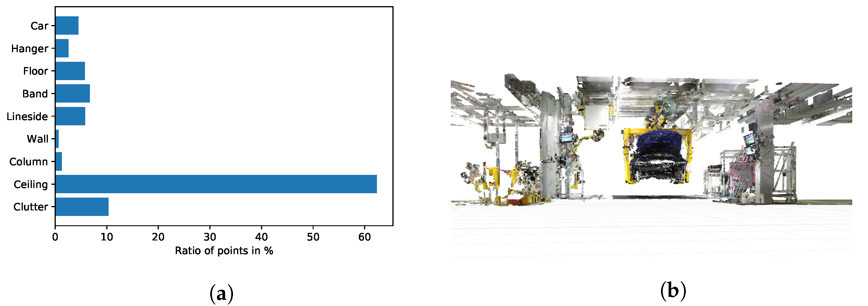
36] with a 25 mm fixed focal length lens were used. We generate a global point cloud comprising 13 tacts of car body assembly by the registration of several smaller point clouds collected at each scanner position. The final point cloud comprises more than one billion points before further pre-processing. The cleaning process is achieved using noise filters for coarse cleaning and fine tuning is done by hand. The resulting point set consists of 594,147,442 points. This accounts for a reduction of approximately 40% of the points after point cloud cleaning. Most of the removed points are noise points that are caused by reflections and the blur of moving objects, like people walking by the laser scanner. The data set is divided into nine different classes, namely car, hanger, floor, band, lineside, wall, column, ceiling, and clutter. The labelling is manually done by the authors. The class clutter is a placeholder for all of the objects that cannot be assigned to one of the other classes. All of the remaining classes are either building structures or objects that can only be moved with high efforts; thus, they are essentially immovable and have to be considered during the planning tasks. The resulting data set is highly imbalanced with respect to the class distribution.
Figure 3a depicts the class distribution of this data set. Clearly, there is a notable excess of points that belong to the class ceiling and relatively few points belong to the classes of wall and column. This is mainly due to the layered architecture of the ceiling that results in points that belong to the structure on various heights. Because walls and columns are mostly draped with other objects, like tools, cables, fire extinguishers, posters, and information signs, there is only a small number of points that truly belong to the classes of wall and column. This is also the reason why especially these two classes suffer from a high degree of missing data, i.e., holes in the point cloud. Any segmentation system has to cope with this class imbalance due to this inhomogeneous class distribution.
Figure 3b illustrates the point cloud of one tact of car body assembly.
5. Results and Analysis
The proposed networks are evaluated on our custom automotive factory data set as well as the scientific data set S3DIS. The segmentation performance is measured with respect to their accuracy and the mean intersection over union. Further, the described ways of uncertainty quantification are evaluated in terms of accuracy after disregarding uncertain predictions. All of the considered models are implemented using Python’s open source library PyTorch [
37]. The input point clouds comprising rooms or assembly tacts are cut into blocks and the number of points within these blocks is sampled to 4096. These blocks serve as input for all networks. All of the models are trained using mini-batch stochastic gradient descent with a batch size of 16 on the S3DIS and the automotive factory data set for the frequentist and the proposed dropout and Bayesian networks. The momentum parameter is set to
for all the models. A decaying learning rate
is used with an initial learning rate of
in the frequentist and the dropout model, as well as
in the Bayesian model. The learning rate is decayed every 10 epochs by a factor of
during frequentist and dropout training, as well as
during Bayesian training. The batch size and the learning rate are optimized by using grid search and cross-validation. In the approximate Bayesian neural network, dropout is applied before the last three convolutional layers and the dropout rate is set to
for the automotive factory data set. In the case of the S3DIS data set, dropout is only applied before the last convolutional layer with a dropout rate of
. Because we do not have dedicated prior information for the Bayesian model, the prior indicates that the parameter values should not diverge. Thus, we choose a prior expectation of zero for all parameters and a standard deviation of 4 and 8 for all weights and biases, respectively. In terms of approximating the posterior predictive distribution, we draw
Monte Carlos samples. All of the considered models converge and training is stopped after 100 epochs.
5.1. Segmentation Accuracy
The three architectures, i.e., the frequentist, dropout, and Bayesian PointNet, as described in
Section 3, are evaluated in the following. The accuracy and the mean Intersection over Union (IoU) are the evaluation metrics used. The accuracy is calculated by the number of correctly classified points divided by the total number of points. The IoU or Jaccard coefficient describes the similarity between two sets with finite cardinality. It is defined by the number of points of the intersection, divided by the number of points of the union of the two sets. In this case, we evaluate the overlap between the points classified as class
i by the model and the points of class
i in the ground truth. Thus, the IoU for class
i reads
where
indicates the class label. The mean IoU is calculated as the mean IoU value over all classes.
Table 1 illustrates that Bayesian PointNet clearly surpasses the performance of frequentist and dropout PointNet with respect to accuracy as well as mean IoU on the test set of both the data sets. Bold table entries represent best model performance in the respective setting and are used throughout the remainder of this section.
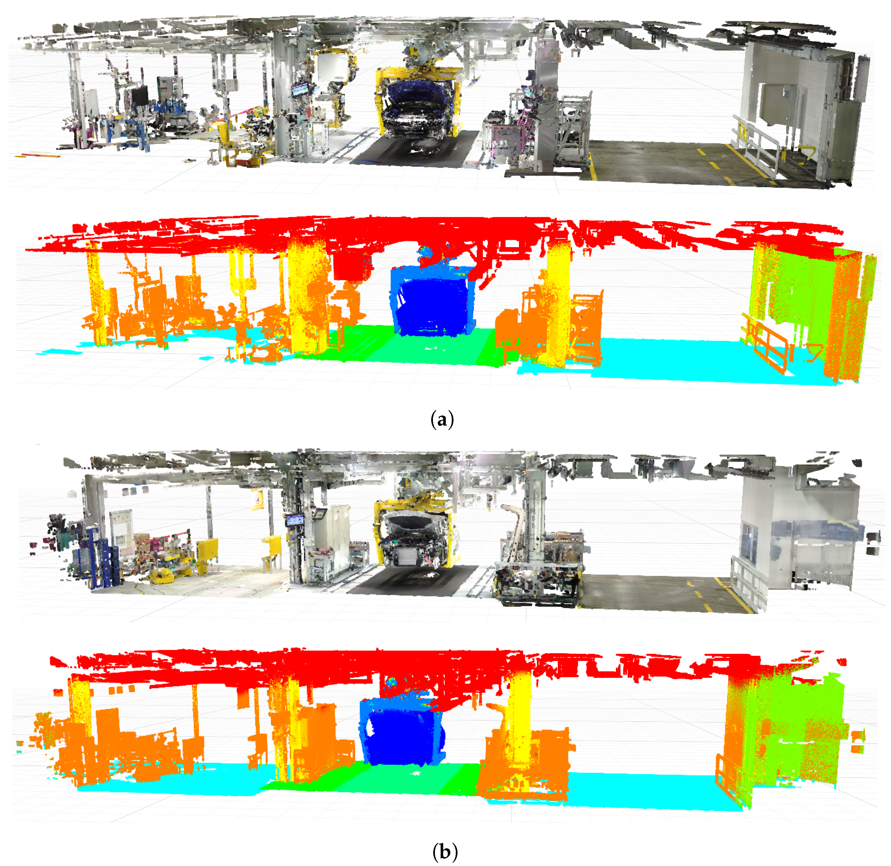
For the S3DIS data set, we test the models on area 6 and, for the automotive factory data set, we set aside two distinct assembly tacts. It is noticeable that all of the models have a higher tendency to overfit on the S3DIS data set than on the automotive factory data set. This is due to the nature of the data itself. While there is a considerable variability between the different areas and room types in the S3DIS data set, there is less variability between the tacts of an assembly plant. They are all designed in a similar way in order to ensure the efficient execution of the assembly process. Even though distinct tacts are used for model training and testing, the variability between the training and test set is much smaller than in the case of the S3DIS data set.
Figure 4 illustrates the qualitative segmentation results for the two automotive tacts in the test set. Clearly, the network generates smooth predictions, with most of the mistakes affecting the classes of column, wall, clutter, and ceiling, which meets our assumption of
Section 4.2. The prior information in the Bayesian model acts as additional observations and, thus, is able to reduce overfitting and increase model performance. An even more striking difference in performance is illustrated in the next section when the information that is provided by uncertainty estimation is considered.
5.2. Uncertainty Estimation
We estimate uncertainty using an entropy based approach, the predictive variance, as well as an approach based on estimating credible intervals on the probabilistic network outputs, as already mentioned. Predictive and aleatoric uncertainty are calculated, as suggested in the Equations (
15) and (
16). Epistemic uncertainty is the difference of these two quantities. The predictive variance is determined on the basis of
forward passes of the input through the network using the unbiased estimator for the variance. Based on the same sample, the 95%-confidence intervals of the network outputs for each class are calculated.
Table 2 contains the results of Bayesian PointNet for one room of each room type in area 6 of S3DIS data set as well as one tact of car body assembly belonging to the test data set. The leftmost column contains the accuracy of Bayesian PointNet. The next column contains the accuracy when only considering predictions that have a predictive uncertainty smaller or equal to the mean predictive uncertainty plus two sigma of the predictive uncertainty. The same is displayed in the next columns with respect to aleatoric and epistemic uncertainty, as well as the variance of the predictive network outputs. In the last column, the predictions for which the 95%-credible interval of the predicted class overlaps with no other class’ 95%-credible interval are considered certain and retained for generating a factory model. It can be seen that the accuracy increases considerably when only looking at certain predictions with respect to any of the uncertainty measures. Generally, the results for predictive and aleatoric uncertainty as well as the credible interval based method are most promising. This confirms our notion that the predictive uncertainty value is mainly determined by aleatoric uncertainty after thorough network training.
Table 3 displays the percentage of predictions, which are found to be uncertain.
Generally, approximately 3% to 11% of the predictions are dropped using the above parameters. The number of dropped predictions decreases when predictions with a higher uncertainty value are considered, e.g., all of the predictions with uncertainty greater or equal to the mean uncertainty plus three sigma. Generally, it can be claimed that the lower the threshold for uncertain predictions, i.e., the more predictions are dropped, the higher the resulting accuracy. Thus, a trade-off between dropping uncertain predictions and segmentation accuracy needs to be found. However, this is largely dependent on the specific use case.
Table 4 illustrates the results of dropout PointNet for one room of each room type in area 6 of S3DIS data set, as well as one tact of car body assembly belonging to the test data set. The accuracy of Bayesian PointNet surpasses the accuracy of dropout PointNet for most of the evaluated rooms.The results are similar in terms of the percentage of predictions dropped.
Table 5 presents the percentage of disregarded predictions as compared to the baseline containing all of the predictions. Again, approximately 2% to 11% of the predictions are dropped by dropout PointNet using the same uncertainty threshold, as before.
Dense point clouds are usually generated, when building up an environment model of a factory in order to capture as many details as possible. Thus, it is important to keep a high number point wise predictions after uncertainty estimation in order to generate a high quality factory model. However, a higher prediction accuracy in the segmentation step also increases the quality of the resulting environment model. A higher accuracy can be achieved by dropping a higher number of uncertain predictions, as we already discussed. In the case of environment modelling, it is vital to drop as few predictions as possible, because, otherwise, building structures and their exact location that is necessary for model generation can get lost.
Generally, we notice that the dropout model is more difficult to train than the Bayesian one, which manifests in a higher epistemic uncertainty in the dropout model. Empirically, it is shown that the application of dropout exhibits inferior performance in convolutional architectures [
3], which could lead to the increased epistemic uncertainty values. Further, the impact of uncertainty on the segmentation performance is more striking in the Bayesian model. However, for applications where one or two percent of accuracy can be sacrificed, the dropout model is a good alternative to the Bayesian model, as users can take on a frequentist network and just add dropout during training and test time, without having to define and optimize a distribution over all the network parameters.
Overall, it can be concluded that Bayesian PointNet has superior performance and dropout PointNet has similar performance to the frequentist model without considering uncertainty information. When only considering certain predictions, Bayesian, as well as dropout PointNet, clearly surpass the performance of the frequentist model. In terms of uncertainty measure, the best results are achieved when using the approach using confidence intervals as well as predictive or aleatoric uncertainty. However, the confidence interval based method drops considerably more predictions in some of the examples.
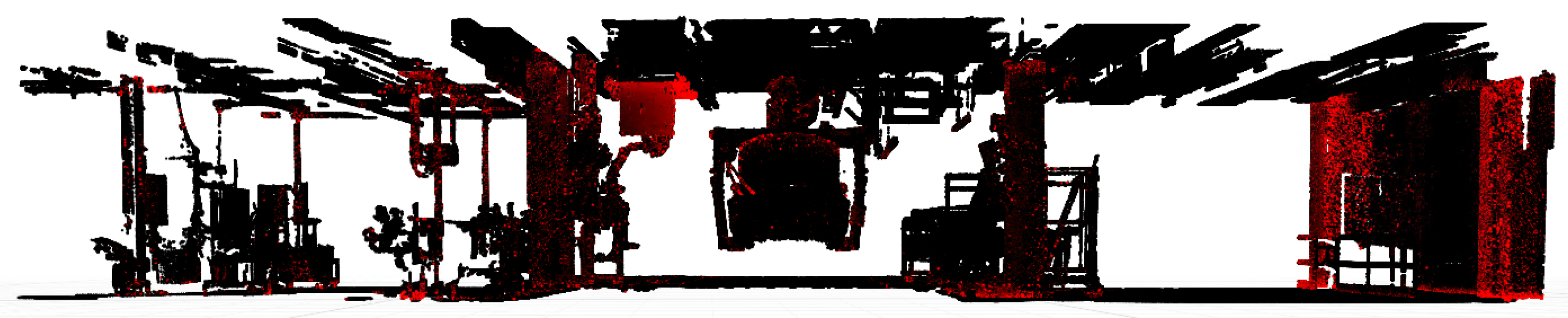
Figure 5 displays one tact of car body assembly, where certain predictions are displayed in black and uncertain predictions are displayed in red. The applied model corresponds to Bayesian PointNet with the credible interval based uncertainty measure. It shows that the network is certain about the majority of its predictions. Uncertain predictions are concentrated at the ceiling, wall, and columns, which is in line with our expectations of
Section 4.2. Because the ceiling, but especially the walls and columns, are hung with clutter objects, this leads to uncertain predictions, as the point clouds of these classes are incomplete due to holes.
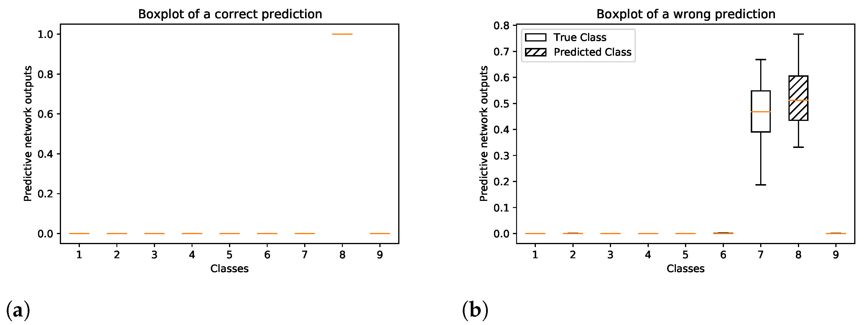
Figure 6 shows the boxplots of the predictive softmax outputs of the Bayesian model for a correct and wrong prediction of two single points in the automotive factory data set. In
Figure 6a, it can be seen that the network is certain about its correct prediction, i.e., all of the predictive softmax output values of the correct class are close to one, while the network outputs for all other classes are close to zero. In the case of a wrong prediction, see
Figure 6b, the boxes of the true and predicted label overlap, which indicates an uncertain prediction. The white box corresponds to the correct class and the shaded box corresponds to the wrongly predicted class.
6. Discussion and Conclusions
We describe how Bayesian segmentation can be applied in order to facilitate the factory planning process in large-scale automotive assembly plants and how to make use of the uncertainty information that is gained by the Bayesian approach. The described use case focuses on the generation of an environment model on the basis of raw point clouds in order to determine the as-is state of a production plant. Therefore, we present a novel Bayesian neural network that is capable of 3D deep semantic segmentation of raw point clouds. This approach allows for the estimation of the uncertainty in the network predictions. Additionally, a network using dropout training to approximate Bayesian variational inference in Gaussian processes is described and compared to the Bayesian model, as well as to a frequentist baseline. In order to evaluate the models, the publicly available S3DIS data set and a manually collected data set of an automotive assembly plant are used.
Different measures of uncertainty quantification are contrasted for the Bayesian as well as the approximate Bayesian network. Three different entropy related uncertainty measures are considered, which enable us to distinguish between overall, data and model related uncertainty. Further, uncertainty quantification based on the variance and credible intervals on the network outputs are investigated. The Bayesian and the dropout model both effectively increase the network performance during test time when compared to the frequentist framework when taking the information gained by any of the uncertainty measures into account. The dropout model’s performance is on-par with the frequentist baseline without taking network uncertainty into account. However, the Bayesian neural network outperforms the frequentist baseline, even without considering uncertainty. It is more robust against overfitting and allows us to work with fewer example data, due to prior information acting like additional observations, while the computational complexity basically stays the same.
The use of Bayesian neural networks instead of frequentist ones enables the quantification of network uncertainty. On the one hand, this leads to more robust and accurate models. On the other hand, in safety critical applications, uncertain predictions can be identified and treated with special care. For instance, uncertain predictions can be handed to a human operator for further treatment or trigger a pre-defined safety state. Autonomous driving, collaborative robotics, and medical diagnosis are important example applications, where uncertainty quantification plays a major role. However, many other domains without safety criticality can profit from determining network uncertainty as well. For instance, post offices sorting letters according to their ZIP code can process uncertain results with more complex statistical methods that are too time consuming for regular application. Similarly, Bayesian neural networks increase model accuracy in factory planning. However, the formulation of such a Bayesian segmentation network requires in depth mathematical knowledge and it is therefore more difficult to update. Thus, dropout training can be a good alternative, as it enables the quantification of uncertainty, while the network structure and optimization stay the same as in the frequentist model. The estimation of uncertainty information in modelling production sites increases model accuracy and it can lead to more accurate reconstructions of the real-world production system in a simulation engine or in CAD software. However, there is a trade-off between increasing the network’s accuracy by discarding uncertain predictions and having a less accurate model, because too many predictions have been discarded. Therefore, we come to the conclusion that it is better to set a higher threshold for dropping uncertain predictions, i.e., fewer predictions are discarded. There is a slight loss in network accuracy; however, whole objects or building structures can get lost, when too many predictions are discarded. While all of the discussed uncertainty measures are apt for improving network performance, the most promising results are achieved using predictive and aleatoric uncertainty as well as the credible interval based method. Because the former methods allow us to set a distinct threshold for considering predictions as uncertain, which is not possible in the credible interval based method, we conclude that they are best suited for our factory planning use case.
A first methodology for systematic data collection and processing in a large-scale industrial environment was presented in [
2]. On the process side, all of the non-highlighted steps that are illustrated in
Figure 1 are described in more detail in future work, including technology specifications and a mathematical concept for the placement of the segmented objects in an environment model. Further, different digitalization strategies and registration approaches are discussed. Pose estimation is achieved using a clustering based routine paired with different point cloud registration strategies. Further, the economic potential of this approach will be evaluated for an exemplary assembly plant. With respect to mathematical concepts, the Bayesian neural network can be extended in a way that the parameters of the prior distribution of the network weights and biases are not treated as hyper parameters of the network. A separate prior can be placed over the prior parameters in order to estimate these quantities in a Bayesian way. Further, the application of network uncertainty for point cloud cleaning will be evaluated.


