Multiplane Optimizing Phase Holograms Using Advanced Machine Learning Algorithms and GPU Acceleration

Abstract

Phase holography is a critical optical imaging and information processing technique with applications ranging from microscopy to optical communications. However, optimizing phase hologram generation remains a significant challenge due to the non-convex nature of the optimization problem. This paper presents a novel multiplane optimization approach for phase hologram generation to minimize the reconstruction error across multiple focal planes. We significantly improve holographic reconstruction quality by integrating advanced machine learning algorithms like RMSprop and Adam with GPU acceleration. The proposed method utilizes TensorFlow to implement custom propagation layers, optimizing the phase hologram to reduce errors at strategically selected distances.

1. Introduction

Phase holography has revolutionized the generation and reconstruction of three-dimensional images by encoding spatial information through manipulating the light beam’s phase [1]. Generating phase holograms combines optical and computational approaches. A fundamental challenge of traditional optical methods, such as interferometry and diffraction, is that the object must be physically present in the experimental system. This requirement can limit recording capabilities [2]. Holographic recording becomes impractical if the object is inaccessible, too large, or incompatible with laser illumination. Computer-generated holograms (CGH) address this limitation by allowing the generation and manipulation of holograms of any scene or object digitally without requiring its physical presence [3]. This not only removes the restrictions associated with object size and accessibility but also opens up possibilities for applications in scientific visualization, virtual reality, and optical communications, where the flexibility and adaptability of CGHs are essential.

On the other hand, computational methods have gained popularity due to their flexibility and accuracy. These methods use algorithms to calculate the necessary phase to be printed or displayed on a spatial light modulator (SLM) [2,4]. Furthermore, advanced techniques have been developed for precise control of both phase and amplitude in computer-generated holograms, allowing for improved fidelity of three-dimensional reconstruction [5].

Phase holograms are essential because of their applications in fields such as microscopy, metrology, medical visualization, and optical communications [6,7,8]. In this context, optimizing phase hologram generation has become a crucial goal to improve the accuracy and efficiency of these applications, offering new capabilities in three-dimensional image capture and reconstruction [2,9]. In the field of microscopy, digital holography has emerged as an advanced method for phase imaging of semi-transparent and transparent objects. This approach allows for high resolution and contrast in imaging small specimens, facilitating quantitative characterization of the observed objects’ three-dimensional morphology and refractive index [10]. Also, these capabilities have been essential in biomedical and biotechnology studies, where detailed and accurate images are paramount for analysis and diagnosis [11]. Furthermore, digital holography has enabled the integration of confocal and widefield microscopy techniques, further expanding microscopic observation capabilities [12,13]. In medical visualization, phase holography has enabled significant advances in obtaining detailed and accurate images of biological structures. Digital holographic tomography, in particular, has emerged as a tool for capturing high-resolution three-dimensional images for biomedical research and clinical diagnosis; this technique enables the quantitative measurement of optical parameters of samples in the analysis of tissues and cells at the subcellular level [1,14]. The ability of this technology to produce high-quality images in real-time has innovated areas such as image-guided surgery and monitoring of dynamic processes in cellular biology [15]. In metrology, phase holograms have proven helpful for surface measurement and three-dimensional reconstruction of microscopic structures due to their ability to capture both the amplitude and phase of reflected or transmitted light. Relevant in fabricating microelectromechanical devices (MEMS) and inspecting advanced materials [16,17]. Digital holography in optical metrology has facilitated the non-destructive inspection of industrial components, providing data on surface topography and defects at the nanoscale [18]. Finally, phase holograms have become vital for efficiently encoding and decoding information in optical communications. The ability to manipulate the light phase with great precision enables high-speed data transmission, essential for developing advanced communication networks that can handle large volumes of information with low latency and high fidelity [19].

Phase holograms are classified into two types: single-phase and dual-phase. Single-phase holograms exclusively modulate the phase of the incident light to form an image, resulting in an energy-efficient process that is less prone to reconstruction errors. On the other hand, dual-phase holograms decompose a complex-valued hologram into two-phase distributions, combining them to generate a more robust final image. This technique, while practical, often introduces unwanted diffraction orders, requiring filtering to enhance image quality [20,21].

One of the most recognized techniques in computer hologram generation is the Gerchberg-Saxton (GS) algorithm [22], widely used in phase retrieval problems. GS is an iterative algorithm that alternates between the spatial and Fourier domains, adjusting the phase so that the reconstructed intensity matches a desired pattern in a specific plane. Although it has been instrumental in developing digital holography, its objective function is rigid. Usually, it requires a lens to perform the Fourier transform, which limits its flexibility and adaptation in different applications. Variants such as the weighted Gerchberg-Saxton (WGS) [23] introduce weighting schemes to improve convergence, while the hybrid input-output (HIO) method [24] allows adjustments in both phase and amplitude, offering greater robustness. However, these techniques maintain dependencies on fixed optical components and objective functions, which may restrict their applicability in contexts where greater flexibility or specific modifications in optimization are required.

Despite the multiple applications, challenges persist in generating phase holograms due to the non-convex nature of the objective function used in the optimization processes. Non-convex optimization in computational holography poses a significant challenge due to the propensity of stochastic gradient descent (SGD) algorithms to get trapped in local minima, which frequently prevents reaching globally optimal solutions and demands exhaustive tuning of hyperparameters to achieve effective convergence. Although pre-computation methods and including specialized loss functions, such as those based on standard deviation or relative entropy, can mitigate some convergence issues, these approaches still critically depend on the correct selection and tuning of input parameters. The sensitivity of these algorithms to the choice of hyperparameters further exacerbates the problem, as it requires fine-tuning specific to each holographic application, which increases the complexity and development time in synthesizing high-quality holograms. Several works analyze these challenges and propose solutions to generate phase holograms. D. P. Kingma and J. Ba [25] present a new non-convex optimization algorithm that minimizes a custom cost function tailored to specific holographic applications, addressing the problem of local minima and the need for fine-tuning hyperparameters. C. Depeursinge [17] presents a computer-generated hologram (CGH) method that incorporates a precomputation procedure and a standard deviation-based loss function, highlighting the challenges of non-convex optimization and the use of SGD.

Recent advances in multi-plane phase retrieval have significantly improved the capabilities of holographic imaging systems. Descloux et al. [26] introduced a combined multi-plane phase retrieval and super-resolution optical fluctuation imaging method for four-dimensional (4D) cellular microscopy, achieving high-resolution volumetric imaging of dynamic cellular processes. Their approach uses a joint optimization framework that combines phase retrieval across multiple planes with super-resolution techniques, enabling the reconstruction of complex biological structures with improved spatial resolution. Similarly, Huang et al. [27] proposed a dual-plane coupled phase retrieval method for holographic imaging without prior information, which reconstructs waves from complex objects without prior knowledge by leveraging data from two nearby planes. This method improves phase retrieval accuracy and reduces reconstruction artifacts by exploiting the coupling between the two planes, offering improved image quality in holographic systems.

In recent years, deep neural networks have emerged as a powerful tool in hologram generation and optimization, achieving significant advances in reconstruction quality and speed. Shi et al. [28] proposed a deep neural network-based approach to generate photorealistic 3D holograms in real-time, using a deep learning architecture that learns to map 3D scenes to phase holograms directly. This method demonstrates a remarkable improvement in artifact removal and the reconstructed images’ visual quality, opening new possibilities for applications in real-time visualization. On the other hand, Peng et al. [29] introduced neural holography with closed-loop training (camera-in-the-loop), where a neural network is trained using images captured directly from the real optical system. This approach allows the model to learn and compensate for imperfections and non-idealities of the physical system, resulting in highly accurate images.

While these methods focus on phase retrieval techniques to improve image quality, our proposed multi-plane optimization approach differs by targeting the optimization of phase hologram generation itself. By integrating advanced machine learning algorithms, such as RMSprop and Adam, and leveraging Graphics Processing Unit (GPU) acceleration, our method minimizes reconstruction error across multiple focal planes strategically selected during the hologram generation. This improves the robustness and accuracy of holographic reconstructions over a range of depths and enhances computational efficiency by using custom propagation layers implemented within a machine learning framework using TensorFlow and Keras.

Our research addresses this problem by significantly improving the objective function for phase hologram generation. The main contribution of this study is incorporating a modified objective function that minimizes the holographic reconstruction error at three different distances: one before the reference distance, another exactly at the reference distance, and a third after the reference distance. The proposal aims to mitigate the effects of non-convex optimization by providing a more robust and accurate reconstruction of the hologram over the entire range of relevant depths.

The improvement in the objective function leverages the angular spectrum theory and applies it to wave propagation. The angular spectrum theory is fundamental in analyzing electromagnetic wave propagation [30]. The theory allows the decomposition of a wave into components of different propagation directions, known as angular components. Each of these components behaves like a plane wave, which facilitates understanding how complex waves propagate through different media; this technique is instrumental in digital holography, as it allows the modeling and simulation of wavefronts along multiple focus planes [31]. By manipulating the angular spectrum of a hologram, it is possible to tune the phase of the light and improve the fidelity of the three-dimensional reconstruction, which is essential in applications requiring accurate depth representation, such as in holographic tomography [32]. Optimizing the hologram’s phase to minimize errors across multiple focal planes achieves higher fidelity in three-dimensional reconstruction. The proposed approach is particularly relevant in applications with crucial depth accuracy representation, such as holographic tomography and medical visualization.

The primary objective of this study is to develop an improved method for generating phase holograms that minimize reconstruction error across multiple focal planes, not just at a single plane. We aim to:

• Implement advanced machine learning algorithms, specifically RMSprop and Adam, to enhance optimization.
• Employ GPU acceleration, a specialized processor designed for parallel computation, to reduce computational load and improve efficiency in tasks such as data processing and complex calculations.
• Validate the proposed method through numerical simulations.

Our main contributions are:

• We propose a novel multiplane optimization strategy that minimizes reconstruction errors at multiple focal distances. This approach improves the robustness and accuracy of holographic reconstructions.
• We implement advanced optimization algorithms within a machine learning framework using TensorFlow and Keras, which enables efficient computation through GPU acceleration.
• We provide a comprehensive comparison with traditional single-plane optimization methods, demonstrating the advantages of our approach in terms of convergence speed and reconstruction quality.
• We validated the effectiveness of the proposed method through numerical simulations and evaluations of the quality of the reconstructed images.

While experimental validation is essential to demonstrate practical applicability, in this work, we focus on the theoretical foundations and computational modeling of multiplane optimization in phase holography. By establishing a solid theoretical foundation, we lay the groundwork for future experimental investigations, which will be addressed in subsequent studies.

The remainder of this paper is organized as follows: Section 2 covers the theoretical foundations of phase holography and the angular spectrum method. Section 3 discusses the optimization algorithms employed, including their mathematical formulations and relevance to the problem. In Section 4, we describe in detail our approach to multiplane optimization, including specific aspects of its implementation and the computational setup used for execution. Section 5 presents the results, including numerical simulations and experimental verification, followed by a comprehensive discussion. Finally, Section 7 concludes the paper and suggests directions for future research.

2. Fundamentals of Phase Holography

2.1. Phase Holography Principles

Phase holography is an advanced technique in physical optics that allows the three-dimensional reconstruction of images by manipulating the phase of light [33]. Recent advancements, driven by the combination of Fourier optics and artificial intelligence, have significantly improved optical image modeling and processing. This combination allows for accurate mathematical representation of light propagation through complex optical systems [34]. The generation of phase holograms involves modulating the phase of a light beam to encode three-dimensional information, which can be reconstructed through optical propagation techniques. To compute a phase hologram, the incident optical field is mathematically modeled as a complex combination of amplitude and phase, usually described by the equation:

$$U(x,y)=A(x,y)e^{i\varphi (x,y)}$$

(1)

where $A(x,y)$ represents the amplitude of the field and $\varphi (x,y)$ the phase. In computer-generated phase holography, the phase of the hologram is calculated by fitting the function $\varphi (x,y)$ to minimize the error between the simulated reconstruction and the reference image. Iterative methods such as gradient descent commonly perform this optimization, where each iteration adjusts the phase to reconstruct the target image more accurately in the resulting hologram.

This work optimizes phase hologram generation to minimize the error between the reference image and its holographic reconstruction. The reference image $I_{\mathrm{ref}}(x,y)$ is a two-dimensional function that describes the intensity of light at each point in the $(x,y)$ plane. The goal is to generate a phase hologram $H(x,y)$ that, when propagated, reconstruct $I_{\mathrm{ref}}(x,y)$. The phase hologram is mathematically represented as:

$$H(x,y)=exp\left(i\varphi \right(x,y\left)\right)$$

(2)

where $\varphi (x,y)$ encodes the phase information necessary for holographic reconstruction. The quality of the final reconstruction depends on how precisely this phase function is determined. The process involves adjusting $\varphi (x,y)$ so that, when propagated, the reconstructed image, $I_{\mathrm{rec}}(x,y)$, closely matches the $I_{\mathrm{ref}}(x,y)$.

2.2. Angular Spectrum Method

The angular spectrum method is a fundamental tool for modeling the propagation of optical fields, instrumental in the context of phase holography [35]. This phase modulation encodes the reference image’s information in the phase domain. It is essential to examine diffraction theory, particularly Fresnel Diffraction, and the angular spectrum method to understand how phase holograms are generated and optimized. In this theoretical framework, the spatial distribution of the light intensity in the observation plane can be determined accurately using the following mathematical expression:

$$I(x,y,z)={\displaystyle \frac{1}{\lambda z}}{\left|{\int }_{-\infty }^{\infty }{\int }_{-\infty }^{\infty }U(x^{\prime },y^{\prime },0)exp\left({\displaystyle \frac{i\pi ({(x-x^{\prime })}^2+{(y-y^{\prime })}^2)}{\lambda z}}\right)d{x}^{\prime }d{y}^{\prime }\right|}^2$$

(3)

where

• $I(x,y,z)$ is the intensity at the observation plane at coordinates $(x,y)$ at a distance z from the hologram.
• $U(x^{\prime },y^{\prime },0)$ is the complex wave field at the hologram plane, defined at coordinates $(x^{\prime },y^{\prime })$.
• $\lambda$ is the wavelength of the light used.

The above equation is derived from the Huygens-Fresnel principle, which states that each point on a wavefront is a secondary source of spherical waves. The superposition of these secondary waves at a point in the observation plane gives rise to the observed intensity.

Hologram propagation is described by the angular spectrum theory [2]. To understand how the phase hologram propagates information, we use the propagation of light from a hologram plane $z=0$ to an observation plane z can be analyzed using the angular spectrum theory [36]. Let us consider an optical field $U(x,y,0)$ in the plane $z=0$. The Fourier transform to obtain the two-dimensional angular spectrum of this field is defined as:

$$\tilde{U}(f_x,f_y,0)={\int }_{-\infty }^{\infty }{\int }_{-\infty }^{\infty }U(x,y,0)exp\left(-i2\pi (f_{x}x+f_{y}y)\right)dxdy$$

(4)

where

• $\tilde{U}(f_x,f_y,0)$ is the angular spectrum in the plane of the hologram.
• $f_x$ y $f_y$ are the spatial frequencies in the x and y directions, respectively [37].

To calculate the wavefield $U(x,y,z)$ in a plane at a distance z, the inverse Fourier transform is applied to the angular spectrum modified by a spatial transfer filter $STF(f_x,f_y,z)$:

$$U(x,y,z)={\mathcal{F}}^{-1}\left\{\tilde{U}(f_x,f_y,0)·STF(f_x,f_y,z)\right\}$$

(5)

The spatial transfer filter, which incorporates the effect of light propagation through the distance z, is defined as:

$$STF(f_x,f_y,z)=exp\left(-i2\pi z\sqrt{{\displaystyle \frac{1}{{\lambda }^2}}-f_x^2-f_y^2}\right)$$

(6)

This filter modulates each component of the angular spectrum to represent how plane waves propagate in free space. Finally, the intensity of the reconstructed image in the observation plane by squaring the wave field modulus.

$$I(x,y,z)={\left|U(x,y,z)\right|}^2$$

(7)

In conventional holography, the illuminating wavefront, $U_{\mathrm{illum}}(x,y)$ and the reconstructed wavefront, $U_{\mathrm{rec}}(x,y,z)$, are clearly distinguished. The illuminating wavefront acts as the coherent source incident on the hologram, while the reconstructed wavefront results from interference containing the object’s three-dimensional information. However, this process is considerably simplified in computer-generated phase holography since computer simulation allows the field to be propagated using numerical models such as the Fourier Transform or the angular spectrum method, thus avoiding the need for an independent physical wavefront. This fundamental difference between both methodologies can be useful for understanding how the reconstructed wavefront can be computationally controlled without the complexity of the physical setup.

2.3. Challenges in Phase Hologram Optimization

Optimizing phase holograms involves finding a phase distribution $\varphi (x,y)$ that minimizes the difference between the reconstructed image $I_{\mathrm{rec}}(x,y,z)$ and a reference image $I_{\mathrm{ref}}(x,y)$. This error is commonly measured using the mean square error (MSE), which is defined as:

$$\mathrm{MSE}={\displaystyle \frac{1}{N}}\sum _{i=1}^N{\left(I_{\mathrm{ref}}\left(i\right)-I_{\mathrm{rec}}\left(i\right)\right)}^2$$

(8)

where

• $I_{\mathrm{ref}}\left(i\right)$ is the intensity of the reference image at the pixel i.
• $I_{\mathrm{rec}}\left(i\right)$ is the intensity of the reconstructed image at the pixel i.
• N is the total number of pixels in the image [37].

Optimization of $\varphi (x,y)$ is achieved by iterative optimization algorithms such as SGD, which iteratively adjusts hologram parameters such as phase modulations to make the reconstructed image as close as possible to the reference image. The SGD algorithm is especially effective for optimizing phase-only holograms [38], significantly enhancing complex amplitude distribution and reducing reconstruction errors [39]. Additionally, phase-only computer-generated holograms (CGHs) benefit from gradient descent methods, which minimize errors in reconstructed images with fewer iterations than traditional algorithms [40]. Implementation of this methodology allows the generation of phase holograms that accurately reconstruct the reference image. Iterative phase optimization reduces reconstruction error and improves the generated hologram quality.

3. Optimization Algorithms

Optimization is a fundamental concept in mathematics and computer science, playing a pivotal role in improving the performance of models by minimizing or maximizing an objective function [41]. In machine learning and phase holography, optimization algorithms are essential for tuning the parameters of a model, either to fit observed data or improve the reconstruction of a phase hologram, ultimately reducing errors and enhancing performance. The selection of the right optimizer is critical in machine learning models, as it can greatly affect both the convergence speed and the final accuracy. Over the years, various optimization algorithms have been proposed, each offering unique advantages depending on the problem’s structure and complexity. Optimization poses challenges in phase holography due to the problem’s non-convex and high-dimensional nature, requiring algorithms that can efficiently explore the solution space while adapting to the problem’s dynamics.

Regarding the algorithm’s stopping condition, we have set a limit of 3000 iterations without a specific error threshold. The main objective of this approach was to evaluate the convergence capacity of the different algorithms and determine how the proposed strategy reduces the error throughout all iterations. The absence of a minimum error threshold as a stopping condition allowed us to analyze the convergence dynamics in detail without forcing an arbitrary endpoint for the optimization process.

Below, we review some of the most influential algorithms in this field, including their historical context and first uses in the literature. These include SGD, RMSprop, Adam, and Nadam, widely adopted in optimizing deep learning models and showing promising results in phase holography optimization [42].

3.1. SGD

SGD originates in the work of Robbins and Monro in 1951, where it was first introduced as a method to approximate the solution of a stochastic approximation problem [43]. Despite its simplicity, SGD has successfully trained large-scale models, including deep neural networks.

SGD updates the model’s parameters by calculating the gradient of the loss function concerning a single data sample or a small batch instead of using the full dataset. This approach allows for faster updates and greater variability in parameter updates, which can help avoid local minima and lead to better generalization on large datasets [44]. The update rule for SGD is given by:

$${\theta }_{t+1}={\theta }_t-\eta ·{\nabla }_{\theta }J(\theta ;x^{\left(i\right)},y^{\left(i\right)})$$

(9)

where $\eta$ is the learning rate, J is the loss function, and  $x^{\left(i\right)},y^{\left(i\right)}$ represent the input-output pair at the i-th sample. Despite its simplicity, SGD has shown great success in training large-scale models, including deep neural networks [45].

3.2. RMSprop (Root Mean Square Propagation)

RMSprop, introduced by Geoffrey Hinton in a 2012 lecture [46], was designed to address the challenges posed by adaptive learning rates, especially for problems where gradients can vary significantly in magnitude. RMSprop introduces a running average of the squared gradients, which helps to stabilize the learning rate and prevent large oscillations during training [47,48].

The RMSprop update rule is as follows:

• Compute the running average of squared gradients:

  $$E\left[g^2\right]t=\beta E\left[g^2\right]t-1+(1-\beta )g_t^2$$

  (10)
• Update the parameters:

  $${\theta }_{t+1}={\theta }_t-{\displaystyle \frac{\eta }{\sqrt{E{\left[g^2\right]}_t+ϵ}}}{g}_t$$

  (11)

Here, $\beta$ represents the decay rate, and  $ϵ$ is a small constant added for numerical stability. RMSprop is particularly well-suited for optimizing cost functions that exhibit different magnitudes of gradients, a common scenario in phase holography [49].

3.3. Adam (Adaptive Moment Estimation)

Adam, introduced by Kingma and Ba in 2014 [25], is one of the most widely used optimization algorithms today. Adam is known for its efficiency and ability to handle non-stationary objectives [50].

The Adam algorithm adjusts the learning rate based on estimates of the first and second moments of the gradients:

• Update biased first and second moment estimates:

  $$m_t={\beta }_1{m}_{t-1}+(1-{\beta }_1)g_t$$

  (12)

  $$v_t={\beta }_2{v}_{t-1}+(1-{\beta }_2)g_t^2$$

  (13)
• Correct bias in moment estimates:

  $${\widehat{m}}_t={\displaystyle \frac{m_t}{1-{\beta }_1^t}}$$

  (14)

  $$\widehat{v}t={\displaystyle \frac{v_t}{1-{\beta }_2^t}}$$

  (15)
• Update parameters:

  $$\theta t+1={\theta }_t-\eta ·{\displaystyle \frac{{\widehat{m}}_t}{\sqrt{{\widehat{v}}_t}+ϵ}}$$

  (16)

Here, ${\beta }_1$ and ${\beta }_2$ are hyperparameters controlling the decay rates for the moment estimates. At the same time, $ϵ$ prevents division by zero. Adam is known for its efficiency and ability to handle non-stationary objectives [51].

Nadam (Nesterov-Accelerated Adaptive Moment Estimation)

Nadam, introduced by Dozat in 2016 [52], builds on the Adam optimizer by incorporating Nesterov’s Accelerated Gradient (NAG) method, which anticipates the update direction by adding a momentum term [53].

Nadam’s parameter update rules are:

$$m_t={\beta }_1{m}_{t-1}+(1-{\beta }_1)g_t$$

(17)

$$v_t={\beta }_2{v}_{t-1}+(1-{\beta }_2)g_t^2$$

(18)

$${\widehat{m}}_t={\displaystyle \frac{m_t}{1-{\beta }_1^t}}$$

(19)

$$\widehat{v}t={\displaystyle \frac{v_t}{1-{\beta }_2^t}}$$

(20)

$$\theta t+1={\theta }_t-{\displaystyle \frac{\alpha }{\sqrt{{\widehat{v}}_t}+ϵ}}({\beta }_1{\widehat{m}}_t+(1-{\beta }_1)g_t)$$

(21)

where $g_t$ is the gradient, and $\alpha$ is the learning rate. The momentum terms ${\beta }_1$ and ${\beta }_2$ enable Nadam to improve both the speed of convergence and the stability of the learning process.

4. Methodology

4.1. Proposed Multiplane Optimization

Multiplane Optimization in Phase Holography is a proposal designed to improve the accuracy of hologram generation by simultaneously addressing reconstruction errors at multiple distances. Unlike traditional methods that optimize hologram quality in a single plane, this strategy considers multiple propagation planes, ensuring that the hologram maintains high fidelity over a range of key distances. Traditionally, optimization is performed by minimizing the error at a single observation plane located at a distance z from the hologram. However, this approach often limits the reconstruction quality, as it overlooks possible variations in image quality at different propagation distances. To address this limitation, we propose a new multi-plane optimization strategy, which consists of minimizing the error of the reconstructed image at three key distances: $z-d$, z, and $z+d$, where d is an additional distance determined by a previous exhaustive search.

The objective function we propose seeks to minimize the average error at the three selected distances, thus allowing a more robust and accurate holographic reconstruction over a broader range of depths. The objective function proposal is defined as:

$$\underset{\mathrm{Holograma},d}{min}{\mathrm{MSE}}_{\mathrm{total}}={\displaystyle \frac{1}{3}}\left({\mathrm{MSE}}_{z-d}+{\mathrm{MSE}}_z+{\mathrm{MSE}}_{z+d}\right)$$

where

$${\mathrm{MSE}}_z={\displaystyle \frac{1}{N}}\sum _{x,y}{\left(I_{\mathrm{ref}}(x,y)-I_{\mathrm{rec}}(x,y,z)\right)}^2$$

$${\mathrm{MSE}}_{z-d}={\displaystyle \frac{1}{N}}\sum _{x,y}{\left(I_{\mathrm{ref}}(x,y)-I_{\mathrm{rec}}(x,y,z-d)\right)}^2$$

$${\mathrm{MSE}}_{z+d}={\displaystyle \frac{1}{N}}\sum _{x,y}{\left(I_{\mathrm{ref}}(x,y)-I_{\mathrm{rec}}(x,y,z+d)\right)}^2$$

where

• ${\mathrm{MSE}}_z$, ${\mathrm{MSE}}_{z-d}$, and ${\mathrm{MSE}}_{z+d}$ represent the mean square error in the distances z, $z-d$, and $z+d$, respectively.
• $I_{\mathrm{ref}}(x,y)$ is the intensity of the reference image in the coordinates $(x,y)$.
• $I_{\mathrm{rec}}(x,y,z)$, $I_{\mathrm{rec}}(x,y,z-d)$, and $I_{\mathrm{rec}}(x,y,z+d)$ are the reconstructed intensities in the coordinates $(x,y)$ at the distances z, $z-d$, and $z+d$, respectively.
• N is the total number of pixels in the image.

After defining the optimization strategy, it is crucial to establish metrics to evaluate the generated holograms’ effectiveness comprehensively. The distance d is a critical parameter representing the separation between the central plane at a distance z and the adjacent planes at $z-d$ and $z+d$. An exhaustive search was conducted to find the optimal value of d that minimizes the total MSE across these planes. The search range was $1\times {10}^{-5}$ to $1\times {10}^{-4}$ meters, with increments of $1\times {10}^{-5}$ meters. The optimal value was $9\times {10}^{-5}$ meters (90 μm). In multiplane optimization, we calculate the MSE at positions $z\pm d$ using the same target image as at z. This approach seeks to improve the robustness of the hologram against small variations in the axial position of the reconstruction plane. By penalizing the differences between the defocused image at $z\pm d$ and the focused target image, we force the algorithm to find a phase distribution that maintains high reconstruction quality over a range of distances around z. This increases the effective depth of focus and makes the system more tolerant of misalignments or uncertainties in the propagation distance.

4.2. Evaluating Image Quality

In addition to using the MSE as an error measure, we incorporate the Structural Similarity Index Measure (SSIM), and the Peak Signal-to-Noise Ratio (PSNR) to evaluate the quality of the reconstructed images. These metrics provide a comprehensive assessment of image fidelity, considering factors beyond simple pixel-wise differences.

• SSIM is a metric designed to measure the perceived similarity between two images, considering changes in luminance, contrast, and structure. It was developed as a direct improvement over the UQI (Universal Quality Index) [54], which already considered these factors but in a more limited way. SSIM introduces key improvements, better aligning with the human perception of visual quality [55]. Mathematically, SSIM for two images $I_{ref}$ and $I_{rec}$ of size $N\times N$ is defined as:

  $$\mathrm{SSIM}(I_{ref},I_{rec})={\displaystyle \frac{(2{\mu }_{I_{ref}}{\mu }_{I_{rec}}+C_1)(2{\sigma }_{I_{ref}{I}_{rec}}+C_2)}{({\mu }_{I_{ref}}^2+{\mu }_{I_{rec}}^2+C_1)({\sigma }_{I_{ref}}^2+{\sigma }_{I_{rec}}^2+C_2)}}$$

  (22)

  where:

  –

  ${\mu }_{I_{ref}}$ and ${\mu }_{I_{rec}}$ are the mean values of images $I_{ref}$ and $I_{rec}$, respectively.

  –

  ${\sigma }_{I_{ref}}^2$ and ${\sigma }_{I_{rec}}^2$ are the variances of $I_{ref}$ and $I_{rec}$.

  –

  ${\sigma }_{I_{ref}{I}_{rec}}$ is the covariance between $I_{ref}$ and $I_{rec}$, calculated as:

  $${\sigma }_{I_{ref}{I}_{rec}}={\displaystyle \frac{1}{N^2}}\sum _{i=1}^N\sum _{j=1}^N(I_{re{f}_{ij}}-{\mu }_{I_{ref}})(I_{re{c}_{ij}}-{\mu }_{I_{rec}})$$

  (23)

  The terms $C_1$ and $C_2$ are constants to avoid instability when the denominators approach zero. SSIM ranges from $-1$ to 1, where 1 indicates structurally identical images.
• PSNR  is a metric based on the pixel-wise intensity differences between two images and is defined as:

  $$\mathrm{PSNR}=10{log}_{10}\left({\displaystyle \frac{MA{X}_I^2}{\mathrm{MSE}}}\right)$$

  (24)

  where $MA{X}_I$ is the maximum possible pixel value of the image (e.g., 255 for 8-bit images), and MSE is the mean squared error between the images. By incorporating these additional metrics, a more comprehensive evaluation of the reconstructed image quality is achieved. This encompasses the average error, structural similarity, and perceived visual quality, allowing for a more precise and detailed analysis of the reconstruction performance.

4.3. Implementation Details

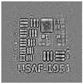
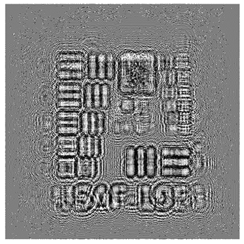
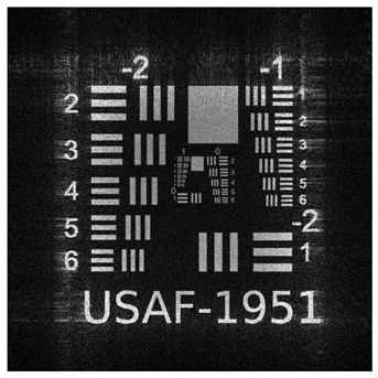
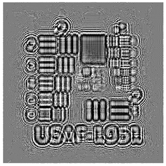
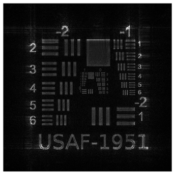
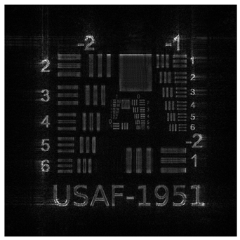
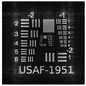
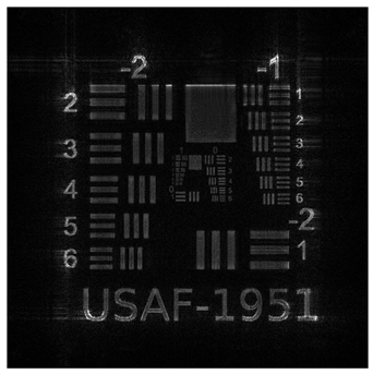
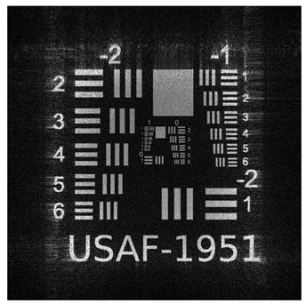
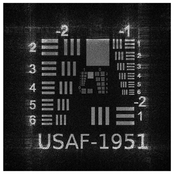
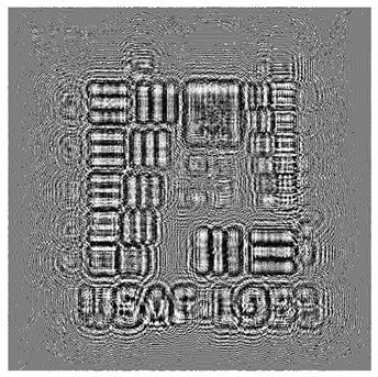
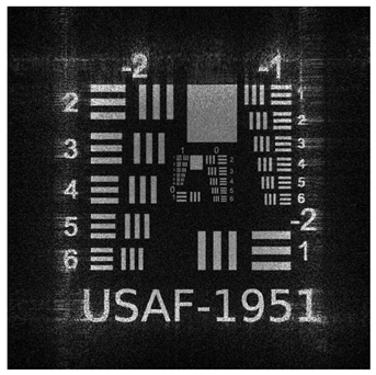
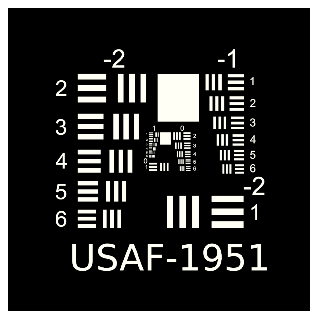
To validate the effectiveness of our multi plane optimization approach, we conducted tests using a widely employed standard pattern in optical system resolution evaluation: the USAF−1951 test chart (Figure 1). This design rigorously assesses the optical system’s ability to resolve details at multiple resolution levels, providing a quantitative measure of the reconstructed image quality [56].

The model utilizes the TensorFlow 2.6 library, integrating an intermediate layer into a neural network to optimize phase hologram generation. The implementation was carried out on an ASUS ROG Strix G16 computer featuring an Intel Core i9-14900HX processor and an NVIDIA GeForce RTX 4060 graphics card with 8 GB of GDDR6 memory and a 128-bit bus. These specifications fully leveraged the machine’s GPU, enabling efficient image processing and training of machine learning models. The software was developed using Python 3.7, CUDA 11.8, and TensorFlow 2.6, all fully compatible with this algorithm’s implementation. The advanced hardware ensures optimal performance on computationally intensive tasks, such as image processing and model parameter tuning during training. The model is evaluated using four optimizers: Adam, Nadam, RMSprop, and SGD. Implementing a holographic layer in TensorFlow simulates holograms propagating across the angular spectrum, and the optimization uses a GPU. During the optimization, the performance of the reconstruction error at the three key distances is evaluated.

The phase of the hologram will be calculated using the angular spectrum method described in the theoretical section. It will be optimized to minimize the error at distances $z-d$, z, and $z+d$. The parameter d is determined through a prior exhaustive search, optimizing the objective function to find the value of d that minimizes the total error across all three distances. The search involves varying d within a predetermined range and calculating the objective function for each case. Finally, it requires selecting the value of d that minimizes the total error for subsequent optimization.

4.4. Experimental Procedure

This study focuses on the proposed multiplane optimization method’s theoretical development and numerical simulation. We systematically analyze the method’s performance and effectiveness under controlled conditions by implementing the algorithms within a computational framework. This approach isolates the optimization strategy’s effects from the confounding variables in experimental setups, offering a clear understanding of the method’s underlying principles and potential benefits.

• Phase Hologram Initialization: We compute the initial phase by performing a backpropagation of the object’s optical field, using an interference simulation between the object and reference wavefronts. This process incorporates structural information from the target image, ensuring a consistent and fair starting point for all optimization algorithms.
• Hologram Propagation: Propagated the hologram using the angular spectrum method at three specific distances: $z-d$, z, and $z+d$.
• MSE Calculation: For each propagated plane, the MSE is calculated between the reconstructed and target images.
• Phase Hologram Update: The phase hologram is updated using the selected optimization algorithm (e.g., Adam, Nadam, RMSprop, or SGD). This step involves iteratively adjusting the hologram’s phase values to minimize the loss function calculated in the previous step.
• Optimization Process Iteration: Steps 2 through 4 are repeated for a predefined number of iterations. This iterative process allows progressive refinement of the phase hologram, improving the reconstruction quality at each step and ensuring the optimization converges to an optimal solution.
• Data Logging: During the optimization process, MSE values and reconstruction images are logged at specific iteration intervals. This systematic logging allows for monitoring the optimization progress, assessing continuous improvement in reconstruction quality, and detecting potential stagnation or premature convergence.

During the reconstruction of holograms, unwanted diffraction orders may appear that can distort the quality of the reconstructed image. In our methodology, the computational model significantly simplifies the problem by considering only the desired diffraction order, omitting the others to simplify the mathematical model, facilitate optimization, and reduce the computational cost. Also, to ensure a fair comparison between the different optimization algorithms, we use an initial phase based on an interference simulation between the object wavefronts and the reference wavefronts. Specifically, we perform a backpropagation of the object’s optical field, considering only the phase resulting from this backpropagation. This approach incorporates structural information of the object in the initial phase, improving the convergence and effectiveness of the optimization algorithms. Mathematically, the initial phase calculation process is described as

$$U(x,y)=exp\left(iI\right(x,y\left)\right)$$

(25)

where $I(x,y)$ is an initial phase assigned based on a reference image. The Fourier transform $\tilde{U}(f_x,f_y)$ is calculated, the backpropagation factor $H(f_x,f_y)=exp\left(-ik{\displaystyle \frac{z}{z_1}}\right)$ is applied, and the backpropagation field $U(x,y,z_1)$ is obtained by the inverse Fourier transform. The initial phase is set as $\mathit{fase} \mathit{inicial}=-arg\left\{U(x,y,z_1)\right\}$. This methodological choice ensures that all optimization algorithms start from the same physical condition, allowing a fair and consistent performance comparison.

Algorithm 1 shows the iterative optimization elements that adjust the hologram phase based on a multiplane loss function, thereby reducing reconstruction errors in three strategic planes. Implementing custom propagation layers in a simple neural network environment facilitates the evaluation of hologram performance in each plane, improving its stability and versatility in different applications. This proposal optimizes reconstruction accuracy at the desired distance and increases the hologram’s resilience to position variations, significantly expanding its applicability.

Algorithm 1 Multiplane Optimization

1: Inputs: 2:    Target image $I_{\mathrm{target}}$ 3:    Source image $I_{\mathrm{source}}$ 4:    Physical parameters: wavelength $\lambda$, distance $z_1$, difference $\delta d$, sizes $N_x$, $N_y$, extents ${\mathrm{ext}}_x$, ${\mathrm{ext}}_y$ 5: Initialization: 6: Compute spacings and coordinates: 7:    $dx\leftarrow {\mathrm{ext}}_x/N_x$,    $dy\leftarrow {\mathrm{ext}}_y/N_y$ 8:    x, y, $f_x$, $f_y$ (spatial coordinates and frequencies) 9: Compute wave number in z: 10:    $k_z\leftarrow \sqrt{{\left({\displaystyle \frac{2\pi }{\lambda }}\right)}^2-f_x^2-f_y^2}$ 11: Define propagation distances: 12:    $z_2\leftarrow z-\delta d$,    $z_3\leftarrow z+\delta d$ 13: Compute transfer functions: 14:    $H_i\leftarrow e^{i{k}_z{z}_i}$, for $i=1,2,3$ 15: Process images to obtain amplitudes: 16:    $A_{\mathrm{source}}\leftarrow \mathrm{Process}\left(I_{\mathrm{source}}\right)$ 17:    $A_{\mathrm{target}}\leftarrow \mathrm{Process}\left(I_{\mathrm{target}}\right)$ 18: Estimate initial phase ${\varphi }_{\mathrm{initial}}$ via inverse backpropagation 19: Optimization: 20: Initialize $\varphi \leftarrow {\varphi }_{\mathrm{initial}}$ 21: for $t=1$ to T do 22:    for $i=1$ to 3 do 23:      Compute field: 24:         $U_i\leftarrow A_{\mathrm{source}}·e^{i\varphi }$ 25:      Propagate field: 26:         $U_i^{\prime }\leftarrow \mathrm{IFFT}2\left(\mathrm{FFT}2\left(U_i\right)·H_i\right)$ 27:      Obtain amplitude: 28:         $I_i\leftarrow \left|U_i^{\prime }\right|$ 29:    end for 30:    Compute loss: $MSE$ 31:    Update phase: 32:       $\varphi \leftarrow \varphi -\eta {\nabla }_{\varphi }L$ (using optimizers: Adam, Nadam, SGD, RMSprop) 33: end for 34: Output: 35:    Optimized phase mask $\varphi$ 36:    Reconstructed images $I_{\mathrm{output}}$ 37:    Metrics report: $MS{E}_z$, $SSI{M}_z$, and $PSN{R}_z$

5. Results and Discussion

This section presents and analyzes the results obtained through numerical and experimental evaluations. It discusses computation times, performs a detailed analysis of the MSE results, compares the proposed and traditional methods, and presents the study’s limitations.

5.1. Numerical Results

The results obtained through numerical and experimental evaluations demonstrate the superiority of multiplane optimization over single-plane optimization in generating phase holograms.

Table 1. Multiplane Optimization: Comparison of holograms and reconstructions using different optimization algorithms in the initial and final iterations.

Optimizer	Initial Iteration		Final Iteration
	Hologram	Reconstruction	Hologram	Reconstruction
Adam
Nadam
RMSprop
SGD

compares the generated holograms and their respective reconstructions using the proposed multiplane optimization in conjunction with the Adam, Nadam, RMSprop, and SGD optimization algorithms. Analyzing each algorithm’s initial and final iterations, we observe progressive improvements in reconstruction quality throughout the optimization process. The MSE values associated with each reconstruction quantify image accuracy, showing how multiplane optimization significantly reduces error compared to initial conditions. It is important to note that while the multiplane optimization approach incorporates additional planes at distances $z-d$, $z+d$, and z to guide the optimization process and enhance algorithm robustness, MSE values presented in Table 1 are based on the reconstructions across all three planes. However, the image shown corresponds only to the central plane at a distance z. The auxiliary planes help prevent the algorithm from falling into local minima and improve the overall solution across different depths. This contributes to a more accurate evaluation of the reconstruction quality at multiple distances. The obtained results demonstrate that, by using the same target image in the $z\pm d$ planes, the optimization produces phase holograms that offer a sharp reconstruction in z and nearby positions. This is evidenced by the reduced sensitivity to blur and the improvement of sharpness in adjacent planes. If we had used out-of-focus target images in $z\pm d$, the hologram would have been optimized to reproduce that blur, which does not improve the reconstruction’s overall quality or the depth of focus.

Additionally, a detailed sensitivity analysis was performed to assess the impact of variations in the distance parameter d on the optimization results. Simulations were conducted by varying d within the range defined previously in Section 4. The results were analyzed using the Mean Squared Error (MSE), identifying the optimal configurations for each optimizer. Figure 2 illustrates these findings, highlighting the optimal d value for each optimizer in the corresponding graphs, providing a clear understanding of how the variability of d affects the accuracy and stability of the optimization results.

Table 2. Single−plane Optimization: Comparison of holograms and reconstructions using different optimization algorithms in the initial and final iterations.

Optimizer	Initial Iteration		Final Iteration
	Hologram	Reconstruction	Hologram	Reconstruction
Adam
Nadam
RMSprop
SGD

shows the results obtained with traditional single-plane optimization, comparing the holograms and their reconstructions for the same algorithms. As in Table 1, the initial and final iterations are presented, allowing us to observe the evolution in the reconstruction quality throughout the optimization.

Table 3. Comparison of Initial and Final Values for Single-plane and Multiplane by Optimizer and Metrics: SSIM, PSNR, and MSE.

Metric	Optimizer	Single-Plane		Multiplane
		Initial	Final	Initial	Final
SSIM	Adam	0.1700	0.1813	0.1708	0.1881
	Nadam	0.1568	0.1485	0.1516	0.1605
	RMSprop	0.1832	0.1913	0.1881	0.1952
	SGD	0.1471	0.1673	0.1561	0.1750
PSNR	Adam	8.48 dB	9.04 dB	8.54 dB	9.40 dB
	Nadam	5.51 dB	7.55 dB	5.62 dB	7.98 dB
	RMSprop	9.14 dB	9.58 dB	9.40 dB	9.80 dB
	SGD	5.36 dB	7.26 dB	5.53 dB	8.19 dB
MSE	Adam	9235.38	8104.33	9106.28	7467.77
	Nadam	18,267.56	11,420.10	17,827.60	10,350.21
	RMSprop	7924.59	7161.97	7470.92	6813.11
	SGD	18,931.69	12,211.42	18,188.67	9853.55

shows a detailed analysis of quality metrics in reconstructed images for different optimizers in single-plane and multi-plane configurations, both in their initial and final stages. The metrics include SSIM, PSNR, and MSE values, comprehensively evaluating each method’s performance. The results highlight the limitations of single-plane optimization, which is restricted to a single distance z and, therefore, less effective in depth-variant contexts. In contrast, multi-plane optimization achieves significant improvements in MSE and other metrics. This comparison underscores the differences between the two methodologies, emphasizing how multi-plane optimization enables more robust and faithful reconstruction by capturing depth changes effectively.

In the initial iterations, all algorithms show limited reconstruction quality with high MSE values: Adam (9106.28), Nadam (17,827.60), RMSprop (7470.92) and SGD (18,188.67) in the multi-plane optimization. However, as the iterations progress, a notable error reduction is observed, especially in the multi-plane proposal, where MSE values decrease significantly: Adam (7467.77), Nadam (10,350.21), RMSprop (6813.11) and SGD (9853.55). This consistent and significant reduction in error in the multi-plane optimization confirms its reliability in offering a more accurate reconstruction when considering depth variations.

Although the reduction in MSE for the Adam and RMSprop algorithms is around 10%, it is important to recognize that in phase holography even small decreases in error can result in appreciable improvements in the quality of the reconstructed image. The sensitivity of holographic systems to phase variations implies that small corrections can significantly improve focusing and image sharpness and reduce artifacts such as speckles.

The graph in Figure 3 shows the evolution of the loss function during 3000 iterations for each of the algorithms evaluated under the single-plane and multi-plane configurations. It is observed that the Adam and RMSprop algorithms with the multi-plane configuration reach the lowest loss values and stabilize quickly. This pattern confirms the multi-plane optimization’s ability better to capture the variations in the reconstruction across different depths, resulting in faster and more effective convergence. Additional metrics, such as the Structural Similarity Index (SSIM) and Peak Signal Noise Ratio (PSNR), were computed further to evaluate the improved quality of the reconstructed images. The results in Table 3 show that multi-plane optimization achieves higher SSIM and PSNR values than single-plane optimization. This indicates better structure preservation and noise reduction in the reconstructed images, corroborating the effectiveness of the proposed approach beyond that reflected by MSE alone.

5.2. Computing Times

Table 4. Execution time per optimizer.

Optimizer	Single-Plane		Multiplane
	CPU	GPU	CPU	GPU
Adam	131.03 ms	3.25 ms	191.82 ms	11.44 ms
SGD	130.84 ms	3.16 ms	190.36 ms	11.46 ms
RMSprop	138.57 ms	3.26 ms	199.48 ms	11.54 ms
Nadam	150.44 ms	3.98 ms	214.85 ms	11.97 ms

analyzes the execution times for the algorithms evaluated on CPU and GPU under single- and multi-plane configurations. Note that the multi-plane optimization by evaluating the objective function at multiple distances increases the computation times on both platforms. On GPU, the execution times are multiplied by approximately a factor of 3.5 compared to the single-plane configuration, with Nadam being the most affected algorithm (11.97 ms), followed by RMSprop (11.54 ms). Although this increase in computation time represents a challenge, the times are still reasonable and manageable for practical applications, especially when using accelerated hardware such as GPUs.

Although the differences in computational times per iteration between the evaluated algorithms may seem insignificant (e.g., a difference of 60 ms), it is essential to consider the cumulative effect over the entire optimization process. Our tests optimized each phase hologram over 3000 iterations to ensure proper convergence and high reconstruction quality. This implies that a difference of 60 ms per iteration results in a total increase of 180 s (3 min) in processing time per hologram. In practical applications where optimization of multiple holograms is required or real-time processing is demanded, this cumulative difference significantly impacts the system’s efficiency and viability. Also, the analysis highlights the importance of balancing computational complexity with holographic reconstruction quality. The additional computational time is a justifiable cost in applications with critical image fidelity. Implementation on GPUs allows these times to be significantly reduced while keeping multiplane optimization within practical margins.

6. Limitations and Methodological Considerations in Multi-Plane Optimization for Holographic Reconstruction

While numerical results confirm that multi-plane optimization significantly enhances holographic reconstruction quality compared to single-plane optimization, it is crucial to acknowledge limitations within our theoretical modeling and simulation framework that may affect real-world applicability. The Adam and RMSprop algorithms emerged as particularly robust and effective, achieving the lowest loss and MSE values in simulations and reducing reconstruction error considerably, as illustrated in Figure 3. These findings support the superiority of multi-plane optimization in contexts requiring depth variability. The multi-plane approach remains viable for advanced-phase holography applications despite increased computational time, especially in GPU configurations. The ability of multi-plane optimization to incorporate multiple distances in the objective function allows for a more nuanced capture of light propagation variations, yielding higher fidelity holograms. These results validate the effectiveness of the proposed approach and suggest avenues for further research and optimization. Importantly, our approach shares core principles with the intensity transport technique (TIE), which uses intensity measurements at axially shifted planes to reconstruct phase information [58]. Similarly, by considering field propagation at positions $z\pm d$ and optimizing the hologram to minimize discrepancies with the target image at z, we leverage intensity variations along the propagation axis, enhancing phase estimation and reconstruction robustness. While not directly implementing TIE, this methodology benefits from additional information from neighboring planes, resulting in holograms with improved tolerance to axial variations. Despite these promising theoretical findings, several limitations inherent to our simulations should be considered:

• Absence of Experimental Noise and Systemic Uncertainties: The simulations assume ideal conditions, omitting sources of experimental noise such as thermal fluctuations, electronic noise, mechanical vibrations, and atmospheric turbulence. These perturbations can introduce phase and amplitude fluctuations, leading to potential misalignments and phase errors. For instance, thermal fluctuations can alter the refractive index of the propagation medium, and mechanical vibrations can result in phase distortions. Excluding these factors may lead to overestimating the effectiveness of our multi-plane optimization in practical scenarios.
• Simplifications in the Physical Model: The simulation model simplifies various critical physical phenomena, assuming perfect wave propagation and ignoring higher-order diffraction effects, polarization influences, nonlinear optical responses, and aberrations introduced by optical components. Moreover, we model the spatial light modulator (SLM) as an ideal phase modulator with a continuous phase response, disregarding pixelation, fill factor, phase quantization, and temporal response constraints. Such simplifications can create discrepancies between simulated and experimental results, as these physical factors are known to degrade hologram quality in real implementations.
• Idealized Zero-Order Suppression Assumption: In our simulations, we assume full suppression of the zero-order diffraction beam from the SLM. However, in practice, residual zero-order light is nearly unavoidable due to SLM imperfections and limitations in the optical setup. This residual light may interfere with desired diffraction orders, introducing artifacts and reducing the reconstructed image contrast. Ignoring this effect may lead to an underestimation of reconstruction errors and an overestimation of multi-plane optimization performance.

This comprehensive assessment underscores the strengths and limitations of the proposed multi-plane optimization approach. Recognizing these factors is essential to refine the model further and bridge the gap between simulated and practical applications, advancing the effectiveness and reliability of multi-plane optimization in holographic imaging.

7. Conclusions

This study demonstrates improvements in holographic reconstruction quality. By integrating advanced optical techniques with multiplane optimization algorithms, we achieve better control over the phase distribution, enhancing image definition and clarity. Incorporating deep learning algorithms and GPU acceleration improves image quality and reduces computational load, facilitating complex hologram generation.

Table 5. Advantages and disadvantages of Multiplane Optimization method in Phase Holography.

Advantages	Disadvantages
Higher accuracy	Increased complexity
Robustness across distances	Increased computational cost
Improved versatility	Time-consuming optimization
Comprehensive evaluation	Dependence on prior exhaustive search
Efficient use of resources	Potential for overfitting

shows a comparative analysis of the advantages and disadvantages of this methodology, highlighting benefits such as robustness in reconstruction and comprehensive evaluation across multiple planes, as well as significant challenges related to computational complexity and cost.

Considering both positive aspects and limitations is essential to understand the real impact of this technique and guide future improvements that enhance its applicability in industry and scientific research. The advances achieved through multiplane optimization enhance the fidelity of holographic reconstruction, which could benefit applications such as medical visualization, where three-dimensional accuracy is essential. In optical metrology, capturing fine details at multiple distances can revolutionize the inspection of complex surfaces and advanced materials. In medical visualization, this improved accuracy could facilitate more precise diagnoses and less invasive procedures.

The results underscore the importance of further exploring the convergence between Fourier Optics and Machine Learning techniques. This combination presents a promising avenue for overcoming current challenges in holography. While the advances are significant, addressing these technologies’ scalability and practical implementation in highly complex holographic systems is essential. Future research should further optimize these processes, focusing on industrial and scientific applications that demand precision and adaptability, such as medical visualization and advanced optical communication systems.

8. Future Work

To address the identified limitations, our future work will focus on several key areas:

• Incorporating Realistic Physical Models: We plan to improve our simulations by incorporating more complete physical models that account for experimental noise and system imperfections. This includes modeling the impact of mechanical vibrations, thermal fluctuations, and electronic noise on the phase and amplitude of the optical field. In addition, we will include the effects of SLM features such as finite pixel size, fill factor, phase quantization levels, and temporal response. We seek to better represent the practical system by simulating higher-order diffraction effects and aberrations introduced by optical components.
• Extensive Comparison and Documentation: We will present the experimental implementation, including detailed setup photographs, step-by-step procedures, and side-by-side comparisons of single- and multi-plane optimization results. This approach will thoroughly evaluate the method’s practical applicability and facilitate reproducibility by other researchers.

References

1. Huang, Z.; Cao, L. Quantitative phase imaging based on holography: Trends and new perspectives. Light Sci. Appl. 2024, 13, 145. [Google Scholar] [CrossRef]
2. Poon, T.-C. Digital Holography and Three-Dimensional Display: Principles and Applications; Springer: New York, NY, USA, 2006. [Google Scholar]
3. Sinha, S.; Lee, K.; Li, J.; Barbastathis, G. Lensless computational imaging through deep learning. Optics 2017, 4, 1117–1125. [Google Scholar] [CrossRef]
4. Wang, Y.; Zhang, Z.; Zhao, S.; He, W.; Li, X.; Wang, X.; Jie, Y.; Zhao, C. Structured light reconstruction by Computer-Generated hologram in defect state. Opt. Laser Technol. 2024, 171, 110372. [Google Scholar] [CrossRef]
5. Bowman, D.; Harte, T.L.; Chardonnet, V.; De Groot, C.; Denny, S.J.; Le Goc, G.; Anderson, M.; Ireland, P.; Cassettari, D.; Bruce, G.D. High-fidelity phase and amplitude control of phase-only computer-generated holograms using conjugate gradient minimisation. Opt. Express 2017, 25, 11692–11700. [Google Scholar] [CrossRef]
6. Wang, J.; Chen, J.; Yu, F.; Chen, R.; Wang, J.; Zhao, Z.; Li, X.; Xing, H.; Li, G.; Chen, X.; et al. Unlocking ultra-high holographic information capacity through nonorthogonal polarization multiplexing. Nat. Commun. 2024, 15, 6284. [Google Scholar] [CrossRef]
7. Yamaguchi, I.; Zhang, T. Phase-shifting digital holography. Opt. Lett. 1997, 22, 1268–1270. [Google Scholar] [CrossRef]
8. Schnars, U.; Jüptner, W. Digital recording and numerical reconstruction of holograms. Meas. Sci. Technol. 2002, 13, R85–R101. [Google Scholar] [CrossRef]
9. Shen, C.; Zheng, Y.; Le, Z. Novel approach based on stochastic gradient descent for controlling the reconstructed phase randomness of computer-generated holograms. Opt. Lasers Eng. 2023, 166, 107593. [Google Scholar] [CrossRef]
10. Kemper, B.; von Bally, G. Digital holographic microscopy for live cell applications and technical inspection. Appl. Opt. 2008, 47, A52–A61. [Google Scholar] [CrossRef] [PubMed]
11. Micó, V.; Ferreira, C.; Zalevsky, Z.; Garcia-Monreal, J. Basic Principles and Applications of Digital Holographic Microscopy. In Microscopy: Science, Technology, Applications and Education. 2010. Available online: https://www.researchgate.net/profile/Javier-Garcia-Monreal/publication/266067304_Basic_principles_and_applications_of_digital_holographic_microscopy/links/5527b5900cf2e089a3a1bafc/Basic-principles-and-applications-of-digital-holographic-microscopy.pdf (accessed on 3 July 2024).
12. Liu, C.; Knitter, S.; Cong, Z.; Sencan, I.; Cao, H.; Choma, M.A. High-speed line-field confocal holographic microscope for quantitative phase imaging. Opt. Express 2016, 24, 9251–9265. [Google Scholar] [CrossRef] [PubMed]
13. Bhaduri, B.; Edwards, C.; Pham, H.; Zhou, R.; Nguyen, T.H.; Goddard, L.L.; Popescu, G. Diffraction phase microscopy: Principles and applications in materials and life sciences. Adv. Opt. Photonics 2014, 6, 57–119. [Google Scholar] [CrossRef]
14. Marquet, P.; Depeursinge, C.; Magistretti, P.J. Review of quantitative phase digital holographic microscopy: Promising novel imaging technique to resolve neuronal network activity and identify cellular biomarkers. Neurophotonics 2014, 1, 020901. [Google Scholar] [CrossRef] [PubMed]
15. Wan, M.; Healy, J.J.; Sheridan, J.T. Terahertz phase imaging and biomedical applications. Opt. Laser Technol. 2020, 122, 105859. [Google Scholar] [CrossRef]
16. Pedrini, G.; Faridian, A.; Singh, A.K. Phase retrieval for optical metrology. In Optical Metrology and Inspection for Industrial Applications III, Proceedings of the SPIE/COS Photonics Asia, Beijing, China, 9–11 October 2014; SPIE: Bellingham, WA, USA, 2014; Available online: https://www.spiedigitallibrary.org/conference-proceedings-of-spie/9276/927602/Phase-retrieval-for-optical-metrology/10.1117/12.2071038.short (accessed on 17 July 2024).
17. Depeursinge, C. Digital Holography Applied to Microscopy. In Three-Dimensional Display: Principles and Applications; Springer: Boston, MA, USA, 2006; pp. 65–102. Available online: https://link.springer.com/chapter/10.1007/0-387-31397-4_4 (accessed on 17 July 2024).
18. Fratz, M.; Seyler, T.; Bertz, A.; Carl, D. Digital holography in production: An overview. Light Adv. Manuf. 2021, 2, 15. [Google Scholar] [CrossRef]
19. Kumar, M.; Matoba, O.; Quan, X.; Rajput, S.K.; Awatsuji, Y.; Tamada, Y. Single-shot common-path off-axis digital holography: Applications in bioimaging and optical metrology. Appl. Opt. 2021, 60, A195–A204. [Google Scholar] [CrossRef]
20. Velez-Zea, A.; Barrera-Ramírez, J.F. Double phase computer generated on-axis multiplane holograms. Opt. Lasers Eng. 2023, 169, 107681. [Google Scholar] [CrossRef]
21. Mukherjee, S.; Tanguy, Q.A.A.; Froech, J.E.; Shanker, A.; Boehringer, K.F.; Brunton, S.; Majumdar, A. Partially coherent double phase holography in visible using meta-optics. arXiv 2022, arXiv:2212.01534. Available online: https://arxiv.org/abs/2212.01534 (accessed on 27 August 2024). [CrossRef]
22. Gerchberg, R.W.; Saxton, W.O. A practical algorithm for the determination of phase from image and diffraction plane pictures. Optik 1972, 35, 237–246. [Google Scholar]
23. Zhang, J.; Poon, T.-C.; Kim, K.-S. Region-of-interest-based Gerchberg–Saxton algorithm for three-dimensional object reconstruction. Opt. Lett. 2007, 32, 2967–2969. [Google Scholar] [CrossRef]
24. Fienup, J.R. Phase retrieval algorithms: A comparison. Appl. Opt. 1982, 21, 2758–2769. [Google Scholar] [CrossRef]
25. Kingma, D.; Ba, J. Adam: A Method for Stochastic Optimization. arXiv 2014, arXiv:1412.6980. Available online: https://arxiv.org/abs/1412.6980 (accessed on 7 October 2024).
26. Descloux, A.; Grußmayer, K.S.; Bostan, E.; Lukes, T.; Bouwens, A.; Sharipov, A.; Geissbuehler, S.; Mahul-Mellier, A.L.; Lashuel, H.A.; Leutenegger, M.; et al. Combined multi-plane phase retrieval and super-resolution optical fluctuation imaging for 4D cell microscopy. Nat. Photonics 2018, 12, 165–172. [Google Scholar] [CrossRef]
27. Huang, Z.; Memmolo, P.; Ferraro, P.; Cao, L. Dual-plane coupled phase retrieval for non-prior holographic imaging. PhotoniX 2022, 3, 3. [Google Scholar] [CrossRef]
28. Shi, L.; Li, B.; Kim, C.; Kellnhofer, P.; Matusik, W. Towards real-time photorealistic 3D holography with deep neural networks. Nature 2021, 591, 234–239. [Google Scholar] [CrossRef] [PubMed]
29. Peng, Y.; Choi, Y.; Padmanaban, N.; Wetzstein, G. Neural holography with camera-in-the-loop training. Acm Trans. Graph. (TOG) 2020, 39, 1–14. [Google Scholar] [CrossRef]
30. Wu, Q. Angular spectrum and application in diffraction. J. Wuhan Inst. Chem. Technol. 2006, 26, 45–48. Available online: https://api.semanticscholar.org/CorpusID:124928863 (accessed on 21 August 2024).
31. Anand, A.; Chhaniwal, V.; Javidi, B. Real-Time Digital Holographic Microscopy for Phase Contrast 3D Imaging of Dynamic Phenomena. J. Disp. Technol. 2010, 6, 500–505. Available online: https://opg.optica.org/jdt/abstract.cfm?URI=jdt-6-10-500 (accessed on 31 July 2024). [CrossRef]
32. Su, D.; Wang, X.; Shang, G.; Ding, X.; Burokur, S.; Liu, J.; Li, H. Amplitude-phase modulation metasurface hologram with inverse angular spectrum diffraction theory. J. Phys. D Appl. Phys. 2022, 55, 235102. [Google Scholar] [CrossRef]
33. Khare, K.; Butola, M.; Rajora, S. Fourier Optics and Computational Imaging; Springer: Cham, Switzerland, 2023. [Google Scholar] [CrossRef]
34. Camacho-Bello, C.; Gutiérrez-Lazcano, L.; Ortega-Mendoza, R.M. Artificial intelligence and Fourier optics: Application of DeepLabV3+ in the recovery of a diffracting aperture in light propagation. Rev. Mex. FíSica 2024, 70, 011301. [Google Scholar] [CrossRef]
35. Goodman, J.W. Introduction to Fourier Optics; Roberts and Company Publishers: Greenwood Village, CO, USA, 2005. [Google Scholar]
36. Heimbeck, M.S.; Everitt, H.O. Terahertz digital holographic imaging. Adv. Opt. Photonics 2020, 12, 1–59. [Google Scholar] [CrossRef]
37. Khare, K.; Butola, M.; Rajora, S. Operational Introduction to Fast Fourier Transform. In Fourier Optics and Computational Imaging; Springer International Publishing: Cham, Switzerland, 2023; pp. 51–57. [Google Scholar] [CrossRef]
38. Wang, W.; Wang, X.; Xu, B.; Chen, J. Optical image encryption and authentication using phase-only computer-generated hologram. Opt. Lasers Eng. 2021, 146, 106722. [Google Scholar] [CrossRef]
39. Chen, C.; Lee, B.; Li, N.-N.; Chae, M.; Wang, D.; Wang, Q.-H.; Lee, B. Multi-depth hologram generation using stochastic gradient descent algorithm with complex loss function. Opt. Express 2021, 29, 15089–15103. [Google Scholar] [CrossRef] [PubMed]
40. Liu, S.; Takaki, Y. Optimization of Phase-Only Computer-Generated Holograms Based on the Gradient Descent Method. Appl. Sci. 2020, 10, 4283. [Google Scholar] [CrossRef]
41. Dezsi, E.; Nistor, I.A. Can deep machine learning outsmart the market? A comparison between econometric modelling and long-short term memory. Rom. Econ. Bus. Rev. 2016, 11, 54–73. Available online: https://api.semanticscholar.org/CorpusID:53869368 (accessed on 21 August 2024).
42. Lopez-Betancur, D.; González-Ramírez, E. Evaluation of Optimization Algorithms for Measurement of Suspended Solids. Water 2024, 16, 1761. [Google Scholar] [CrossRef]
43. Robbins, H.; Monro, S. A stochastic approximation method. Ann. Math. Stat. 1951, 22, 400–407. [Google Scholar] [CrossRef]
44. Keras. Stochastic Gradient Descent (SGD) Optimizer. Available online: https://keras.io/api/optimizers/sgd/ (accessed on 10 July 2024).
45. Chen, X.; Lee, J.D.; Tong, X.T.; Zhang, Y. Statistical inference for model parameters in stochastic gradient descent. Ann. Stat. 2020, 48, 251–273. [Google Scholar] [CrossRef]
46. Hinton, G.; Srivastava, N.; Swersky, K. Neural Networks for Machine Learning: Lecture 6a—Overview of mini-batch gradient descent; University of Toronto: Toronto, ON, Canada, 2012; Available online: https://www.cs.toronto.edu/~hinton/coursera/lecture6/lec6.pdf (accessed on 15 August 2024).
47. Keras. RMSprop Optimizer. Available online: https://keras.io/api/optimizers/rmsprop/ (accessed on 9 August 2024).
48. LeCun, Y.; Bengio, Y.; Hinton, G. Deep learning. Nature 2015, 521, 436–444. [Google Scholar] [CrossRef]
49. Xu, D.; Zhang, S.; Zhang, H.; Mandic, D.P. Convergence of the RMSProp deep learning method with penalty for nonconvex optimization. Neural Netw. 2021, 139, 17–23. [Google Scholar] [CrossRef]
50. Keras. Adam Optimizer. Available online: https://keras.io/api/optimizers/adam/ (accessed on 16 August 2024).
51. Soydaner, D. A comparison of optimization algorithms for deep learning. Int. J. Pattern Recognit. Artif. Intell. 2020, 34, 2052013. [Google Scholar] [CrossRef]
52. Dozat, T. Incorporating Nesterov Momentum into Adam. 2016. Available online: https://tdozat.github.io/poster.pdf (accessed on 16 August 2024).
53. Keras. Nadam Optimizer. Available online: https://keras.io/api/optimizers/Nadam/ (accessed on 9 August 2024).
54. Wang, Z.; Bovik, A.C. A universal image quality index. IEEE Signal Process. Lett. 2002, 9, 81–84. [Google Scholar] [CrossRef]
55. Wang, Z.; Bovik, A.C.; Sheikh, H.R.; Simoncelli, E.P. Image quality assessment: From error visibility to structural similarity. IEEE Trans. Image Process. 2004, 13, 600–612. [Google Scholar] [CrossRef] [PubMed]
56. Dwivedi, G.; Sharma, A.; Debnath, S.; Rajkumar. Comparison of numerical reconstruction of digital holograms using angular spectrum method and Fresnel diffraction method. J. Opt. 2017, 46, 12596–12597. [Google Scholar] [CrossRef]
57. Voelz, D.G. Computational Fourier Optics: A MATLAB Tutorial; SPIE Press: Bellingham, WA, USA, 2010; ISBN 978-0-8194-8204-4. [Google Scholar]
58. Alanazi, N.A.; Scott, A.M.; Al-Ghezi, H.; Faryad, M.; Lakhtakia, A.; Banerjee, P.P. Transport of intensity and phase: Applications to digital holography [Invited]. Appl. Opt. 2024, 63, 2436–2454. [Google Scholar] [CrossRef]
Figure 1. USAF −1951 resolution test chart used as the reference image [57].
Optics 05 00041 g001
Figure 2. Sensitivity analysis of multiplane optimization concerning the distance parameter d.
Optics 05 00041 g002
Figure 3. Comparison of the evolution of the loss function during phase hologram optimization using different algorithms and configurations. The graph shows the decrease in error evaluated under both the multi-plane optimization proposal and the traditional single-plane optimization.
Optics 05 00041 g003