Integrated Framework of LSTM and Physical-Informed Neural Network for Lithium-Ion Battery Degradation Modeling and Prediction


Abstract
1. Introduction
- A novel framework is proposed, which integrates LSTM with PINN in a unified manner. The LSTM is employed to extract latent temporal features from battery monitoring sequences, which are then embedded as physical priors into the Deep Hidden Temporal Physical Module (DeepHTPM). This enables more accurate modeling of the degradation dynamics of lithium-ion batteries.
- We propose a dynamic degradation modeling approach based on the chain rule, which leverages early-stage predictions at each LSTM step to impose additional constraints on the model. This enhances reliability, mitigates overfitting in small datasets, and strengthens generalization performance.
- We assess the performance of our framework using the NASA and CALCE datasets. The experimental results show that LSTM-PINN consistently surpasses all baseline models, achieving Mean Absolute Errors (MAEs) of 0.594% on the NASA dataset and 0.746% on the CALCE dataset, along with Root Mean Square Errors (RMSEs) of 0.791% and 0.897%, respectively.
2. Related Works
3. Problem Statement
3.1. Battery Degradation Model
3.2. A Dynamic Model Based on Temporal Features
4. Framework Description
4.1. Framework of LSTM-PINN
4.2. Bayesian Optimization for Hyperparameter Tuning
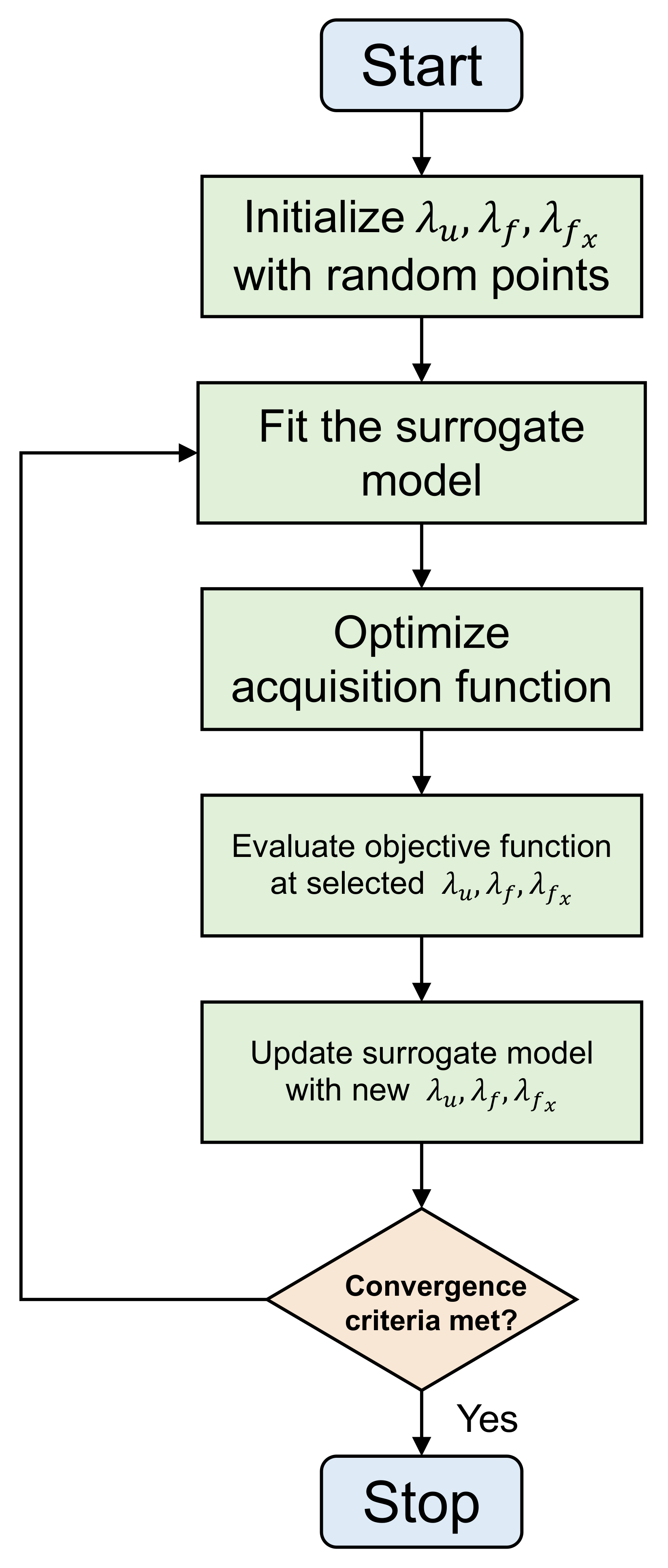
4.2.1. Overview of Bayesian Optimization
- A surrogate model (often a Gaussian process) that approximates the unknown objective function .
- An acquisition function that quantifies the utility of evaluating f at a candidate point .
- Initialize: Select an initial set of hyperparameter points (e.g., via Latin hypercube sampling) and observe .
- Fit Surrogate: Train the surrogate model (e.g., a Gaussian process) on to obtain a posterior distribution , where .
- Optimize Acquisition: Find the next query pointwhere is an acquisition function defined using the posterior predictive mean and variance .
- Evaluate Objective: Compute (training and validating the model with hyperparameters ).
- Augment Data: Update .
- Repeat: Return to Step 2 until a stopping criterion is met (e.g., budget exhausted or convergence).
4.2.2. Algorithmic Summary
| Algorithm 1 Bayesian optimization for hyperparameter tuning |
|
| Algorithm 2 The training process of LSTM-PINN |
|
5. Experiments
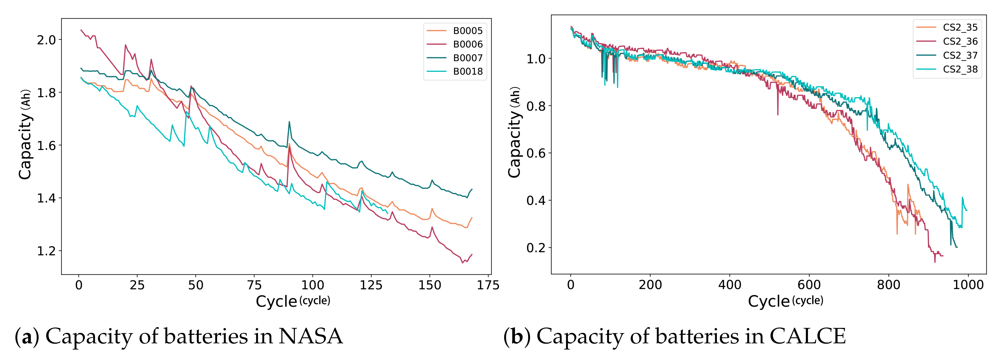
5.1. Dataset Description
5.2. Experiment Results on the NASA and CALCE Datasets
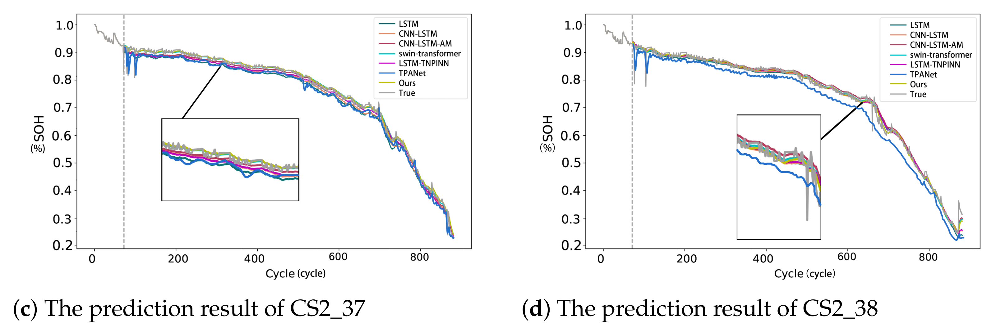
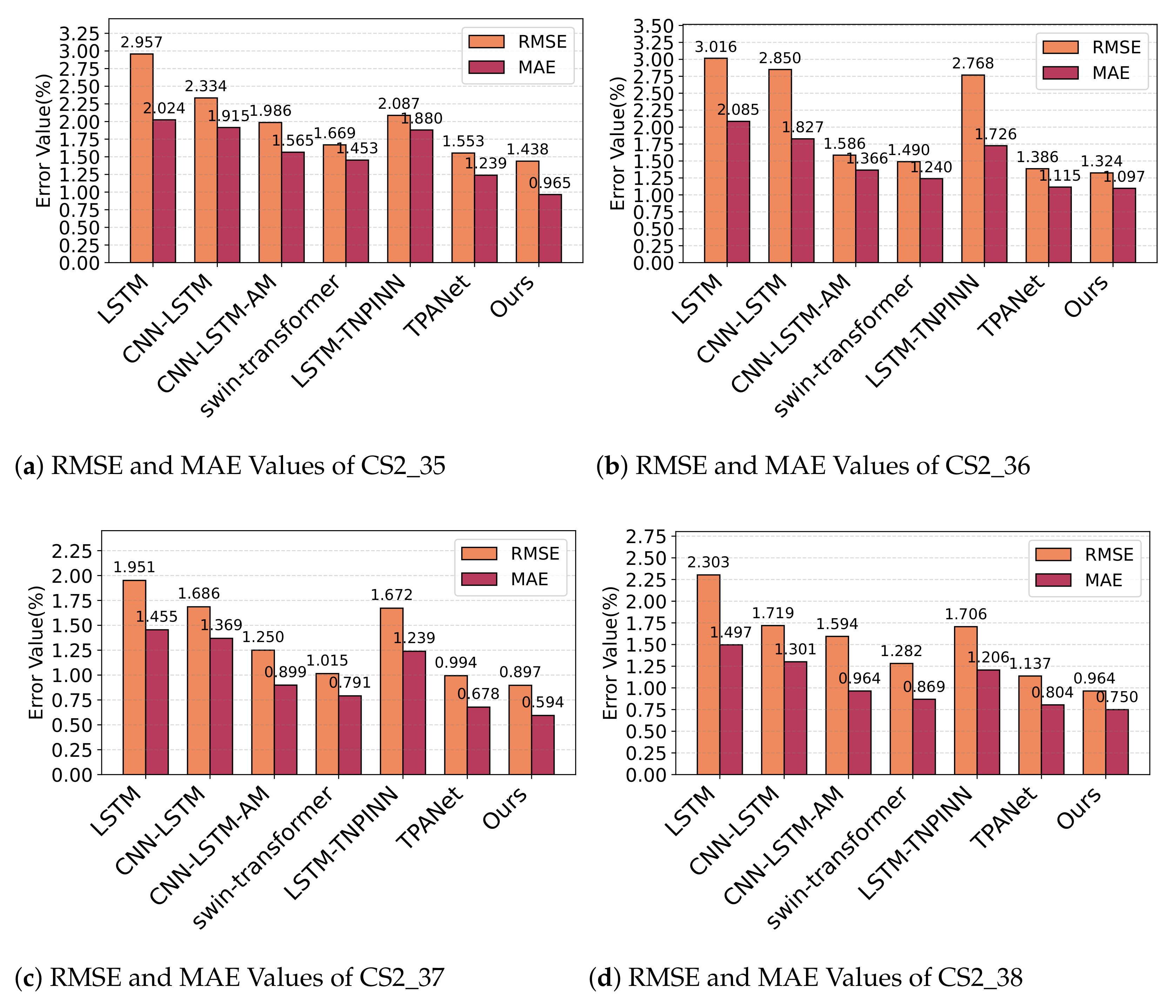
5.2.1. Experiment A
5.2.2. Experiment B
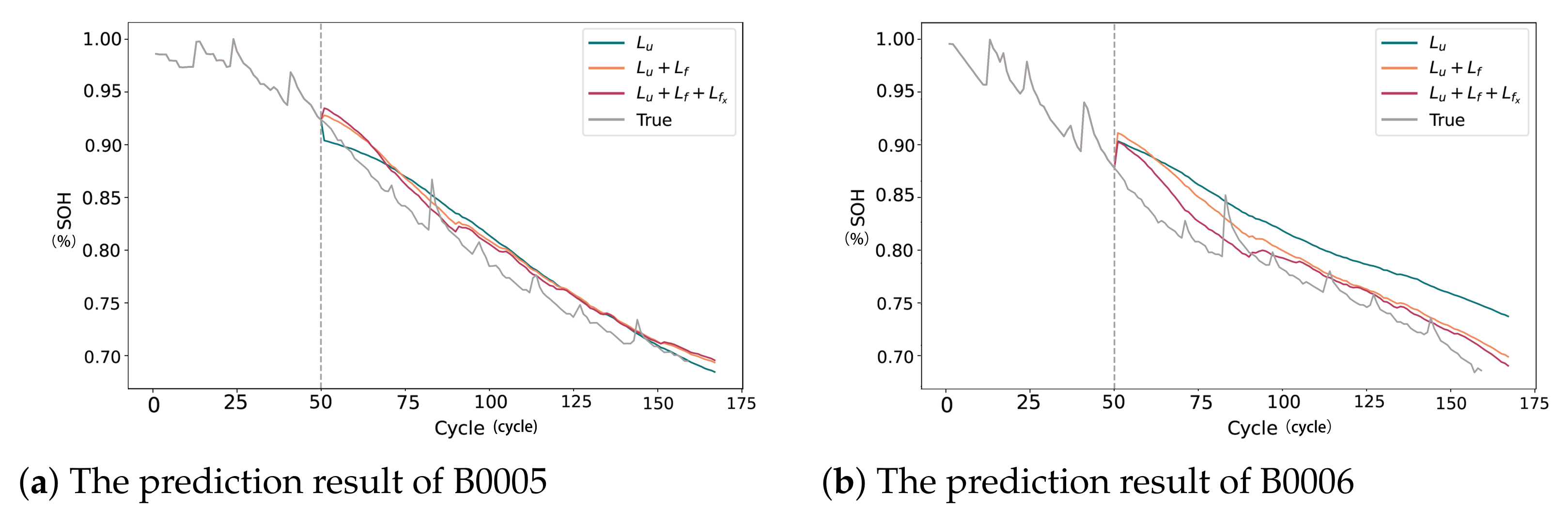
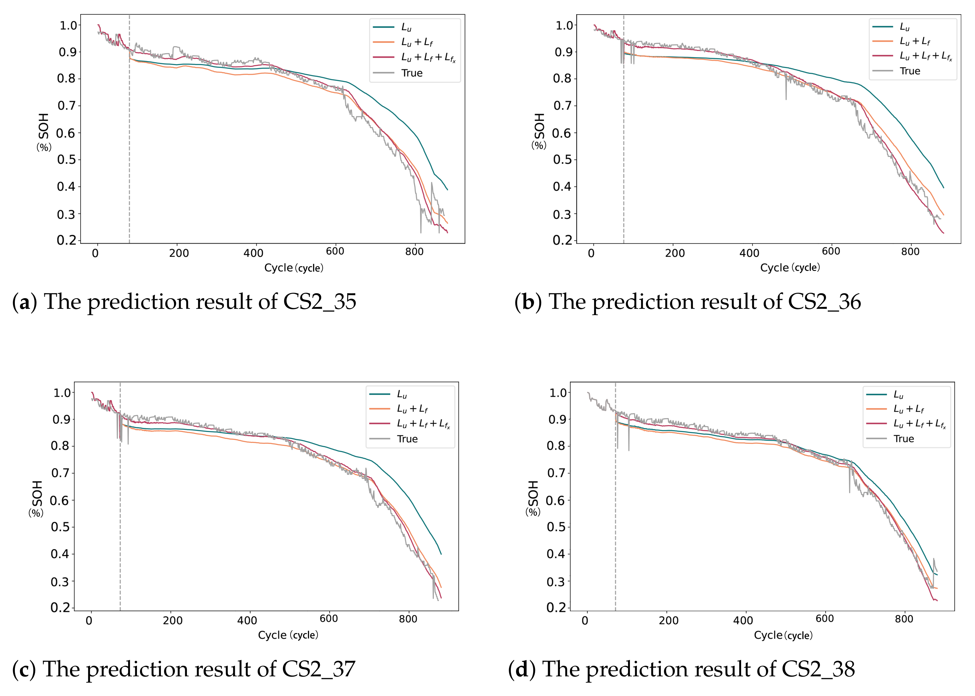
5.2.3. Ablation Study on Different Loss Functions
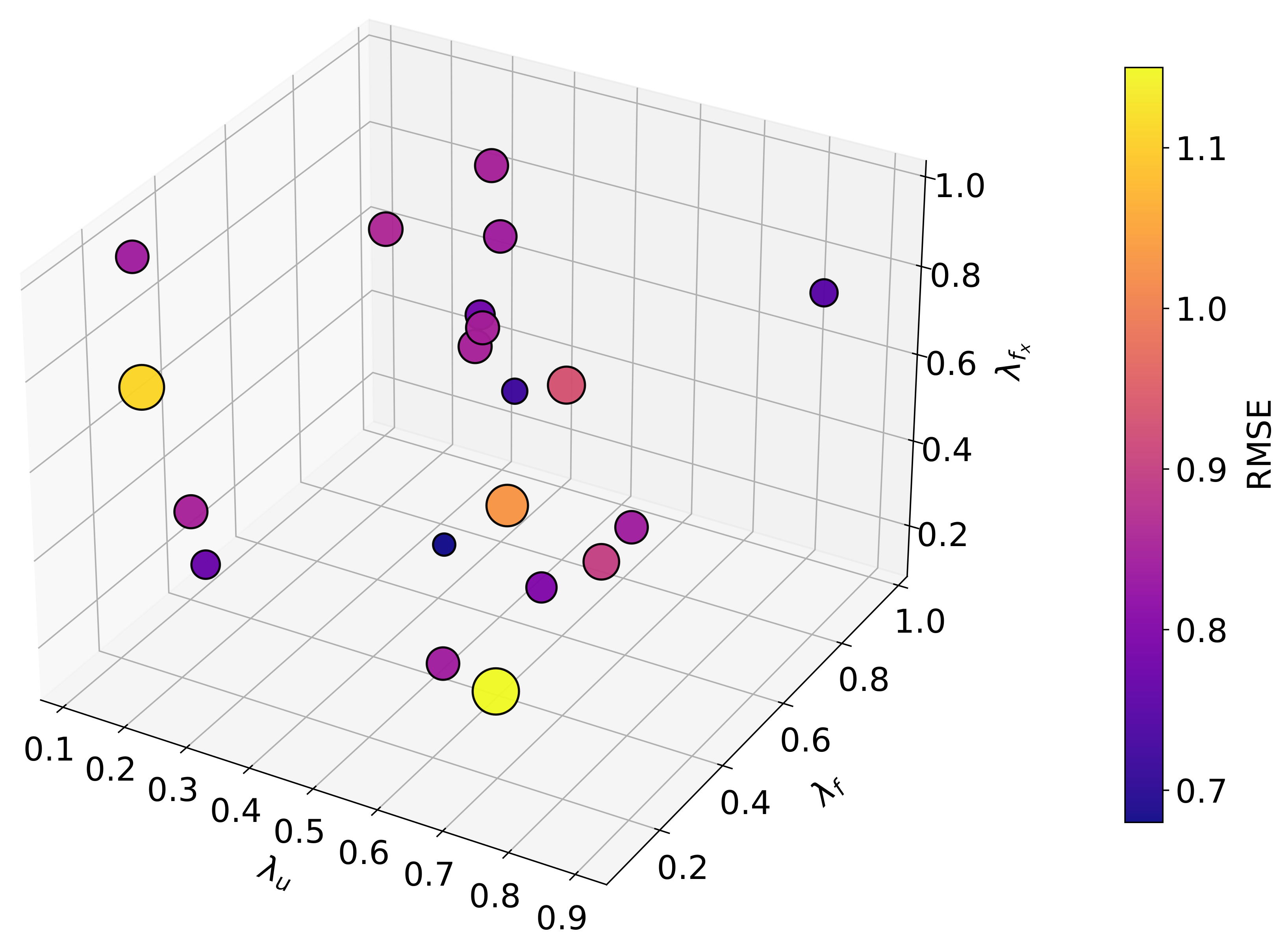
5.3. Impact of Loss Function Weights on Prediction Performance
6. Conclusions
Author Contributions
Funding
Institutional Review Board Statement
Informed Consent Statement
Data Availability Statement
Conflicts of Interest
References
- Wei, Z.; Li, Y.; Cai, L. Electric Vehicle Charging Scheme for a Park-and-Charge System Considering Battery Degradation Costs. IEEE Trans. Intell. Veh. 2018, 3, 361–373. [Google Scholar] [CrossRef]
- Schaut, S.; Arnold, E.; Sawodny, O. Predictive Thermal Management for an Electric Vehicle Powertrain. IEEE Trans. Intell. Veh. 2023, 8, 1957–1970. [Google Scholar] [CrossRef]
- Sarrafan, K.; Muttaqi, K.M.; Sutanto, D. Real-Time State-of-Charge Tracking Embedded in the Advanced Driver Assistance System of Electric Vehicles. IEEE Trans. Intell. Veh. 2022, 5, 497–507. [Google Scholar] [CrossRef]
- Zhao, S.; Chen, S.; Yang, F.; Ugur, E.; Akin, B.; Wang, H. A Composite Failure Precursor for Condition Monitoring and Remaining Useful Life Prediction of Discrete Power Devices. IEEE Trans. Ind. Inform. 2021, 17, 688–698. [Google Scholar] [CrossRef]
- Rincón-Maya, C.; Guevara-Carazas, F.; Hernández-Barajas, F.; Patino-Rodriguez, C.; Usuga-Manco, O. Remaining Useful Life Prediction of Lithium-Ion Battery Using ICC-CNN-LSTM Methodology. Energies 2023, 16, 7081. [Google Scholar] [CrossRef]
- Zhao, S.; Blaabjerg, F.; Wang, H. An overview of artificial intelligence applications for power electronics. IEEE Trans. Power Electron. 2021, 36, 4633–4658. [Google Scholar] [CrossRef]
- Imen Jarraya, S.B.A.; Alahmed, F. SOH-KLSTM: A hybrid Kolmogorov-Arnold Network and LSTM model for enhanced Lithium-ion battery Health Monitoring. J. Energy Storage 2023, 122, 116541. [Google Scholar] [CrossRef]
- Junxiong Chen, W.C.; Zhu, Q. SOC estimation for lithium-ion battery using the LSTM-RNN with extended input and constrained output. Energy 2023, 262, 125375. [Google Scholar] [CrossRef]
- Zhao, S.; Peng, Y.; Zhang, Y. Parameter estimation of power electronic converters with physics-informed machine learning. IEEE Trans. Power Electron. 2022, 37, 11567–11578. [Google Scholar] [CrossRef]
- Qin, L.; Sun, T.; Sun, X.M.; Xia, W. Managing Battery Performance Degradation Using Physics-Informed Learning Scheme for Multiple Health Indicators. IEEE Trans. Transp. Electrif. 2025, 11, 7309–7321. [Google Scholar] [CrossRef]
- Zhang, S.; Liu, Z.; Xu, Y.; Su, H. A Physics-Informed Hybrid Multitask Learning for Lithium-Ion Battery Full-Life Aging Estimation at Early Lifetime. IEEE Trans. Ind. Inform. 2025, 21, 415–424. [Google Scholar] [CrossRef]
- Wang, F.; Zhai, Z.; Zhao, Z.; Di, Y.; Chen, X. Physics-informed neural network for lithium-ion battery degradation stable modeling and prognosis. Nat. Commun. 2024, 15, 4332. [Google Scholar] [CrossRef] [PubMed]
- Yang, F.; Song, X.; Dong, G. A coulombic efficiencybased model for prognostics and health estimation of lithium-ion batteries. Energy 2019, 171, 1173–1182. [Google Scholar] [CrossRef]
- Xu, B.; Oudalov, A.; UIbig, A. Modeling of lithium-ion battery degradation for cell life assessment. IEEE Trans. Smart Grid 2018, 9, 1131–1140. [Google Scholar] [CrossRef]
- Wen, P.; Ye, Z.S.; Li, Y. Physics-Informed Neural Networks for Prognostics and Health Management of Lithium-Ion Batteries. IEEE Trans. Intell. Veh. 2024, 9, 2276–2289. [Google Scholar] [CrossRef]
- Xu, H.; Wu, L.; Xiong, S. An improved CNN-LSTM model-based state-of-health estimation approach for lithium-ion batteries. Energy 2023, 276, 127585. [Google Scholar] [CrossRef]
- Zhun, X.; Zhang, P.; Xie, M. A Joint Long Short-Term Memory and AdaBoost regression approach with application to remaining useful life estimation. Measurement 2021, 170, 108707. [Google Scholar]
- Sherkatghanad, Z.; Ghazanfari, A.; Makarenkov, V. A self-attention-based CNN-Bi-LSTM model for accurate state-of-charge estimation of lithium-ion batteries. Energy Storage 2024, 88, 111524. [Google Scholar] [CrossRef]
- Massaoudi, M.; Abu-Rub, H.; Ghrayeb, A. Advancing Lithium-Ion Battery Health Prognostics With Deep Learning: A Review and Case Study. IEEE Open J. Ind. Appl. 2024, 5, 43–62. [Google Scholar] [CrossRef]
- Sun, H.; Peng, L.; Huang, S. Development of a physics-informed doubly fed cross-residual deep neural network for high-precision magnetic flux leakage defect size estimation. IEee Trans. Ind. Inform. 2022, 18, 1629–1640. [Google Scholar] [CrossRef]
- Cofre-Martel, S.; Droguett, E.L.; Modarres, M. Remaining useful life estimation through deep learning partial differential equation models: A framework for degradation dynamics interpretation using latent variables. Shock Vib. 2021, 2021, 9937846. [Google Scholar] [CrossRef]
- Raissi, M. Deep hidden physics models: Deep learning of nonlinear partial differential equations. J. Mach. Learn. Res. 2018, 19, 932–955. [Google Scholar]
- Kong, J.Z.; Yang, F.; Zhang, X.; Pan, E.; Peng, Z.; Wang, D. Voltagetemperature health feature extraction to improve prognostics and health management of lithium-ion batteries. Energy 2021, 223, 120114. [Google Scholar] [CrossRef]
- Connor, W.D.; Wang, Y.; Malikopoulos, A.A.; Advani, S.G.; Prasad, A.K. Impact of connectivity on energy consumption and battery life for electric vehicles. IEEE Trans. Intell. Veh. 2021, 6, 14–23. [Google Scholar] [CrossRef]
- Liu, H.; Naqvi, I.H.; Li, F. An analytical model for the CC-CV charge of Li-ion batteries with application to degradation analysis. Energy Storage 2020, 29, 101342. [Google Scholar] [CrossRef]
- Severson, K.A.; Attia, P.M.; Jin, N.; Perkins, N. Data-driven prediction of battery cycle life before capacity degradation. Nat. Energy 2019, 4, 383–391. [Google Scholar] [CrossRef]
- Solís-Martín, D.; Galán-Páez, J.; Borrego-Díaz, J. CONELPABO: Composite Networks Learning via Parallel Bayesian Optimization to Predict Remaining Useful Life in Predictive Maintenance. Neural Comput. Appl. 2025, 37, 7423–7441. [Google Scholar] [CrossRef]
- Onorato, G. Bayesian Optimization for Hyperparameters Tuning in Neural Networks. arXiv 2024, arXiv:2410.21886. [Google Scholar]
- Fricke, K.; Nascimento, R.; Corbetta, M.; Kulkarni, C.; Viana, F. An Accelerated Life Testing Dataset for Lithium-Ion Batteries With Constant and Variable Loading Conditions. Int. J. Progn. Health Manag. 2023, 14, 1–12. [Google Scholar] [CrossRef]
- Diao, W.; Naqvi, I.H.; Pecht, M. Early Detection of Anomalous Degradation Behavior in Lithium-Ion Batteries. J. Energy Storage 2020, 32, 101710. [Google Scholar] [CrossRef]
- Lee, C.; Jo, S.; Kwon, D.; Pecht, M. Capacity-Fading Behavior Analysis for Early Detection of Unhealthy Li-ion Batteries. IEEE Trans. Ind. Electron. 2020, 67, 5693–5701. [Google Scholar] [CrossRef]
- Wu, M.; Yue, C.; Zhang, F.; Sun, R.; Tang, J.; Hu, S.; Zhao, N.; Wang, J. State of Health Estimation and Remaining Useful Life Prediction of Lithium-Ion Batteries by Charging Feature Extraction and Ridge Regression. Appl. Sci. 2024, 14, 3153. [Google Scholar] [CrossRef]
- Zhou, K.Q.; Qin, Y.; Lau, B.P.L.; Yuen, C.; Adams, S. Lithium-Ion Battery State of Health Estimation Based on Cycle Synchronization Using Dynamic Time Warping. arXiv 2021, arXiv:2109.13448. [Google Scholar]
- Mirzaee, H.; Kamrava, S. Estimation of internal states in a Li-ion battery using BiLSTM with Bayesian hyperparameter optimization. Energy Storage 2023, 74, 109522. [Google Scholar] [CrossRef]
- Li, W.; Li, Y.; Garg, A.; Gao, L. Enhancing real-time degradation prediction of lithium-ion battery: A digital twin framework with CNN-LSTM-attention model. Energy 2024, 286, 129681. [Google Scholar] [CrossRef]
- Zhang, Z.; Li, M.; Wang, X.; Liu, J. Swin Transformer for State of Charge Prediction of Lithium-Ion Batteries in Electric Aircraft. IEEE Trans. Transp. Electrif. 2025, 12, 645–647. [Google Scholar] [CrossRef]
- Wang, W.; Zhou, Y.; Zhang, L. MCSFormer: A Multi-Channel Swin Transformer Framework for Remaining Useful Life Prediction of Bearings. arXiv 2025, arXiv:2505.14897. [Google Scholar]
- Li, L.; Li, Y.; Mao, R.; Li, Y.; Lu, W.; Zhang, J. TPANet: A novel triple parallel attention network approach for remaining useful life prediction of lithium-ion batteries. Energy 2025, 309, 132890. [Google Scholar] [CrossRef]


| M1 | M2 | M3 | M4 | M5 | M6 | M7 | ||
|---|---|---|---|---|---|---|---|---|
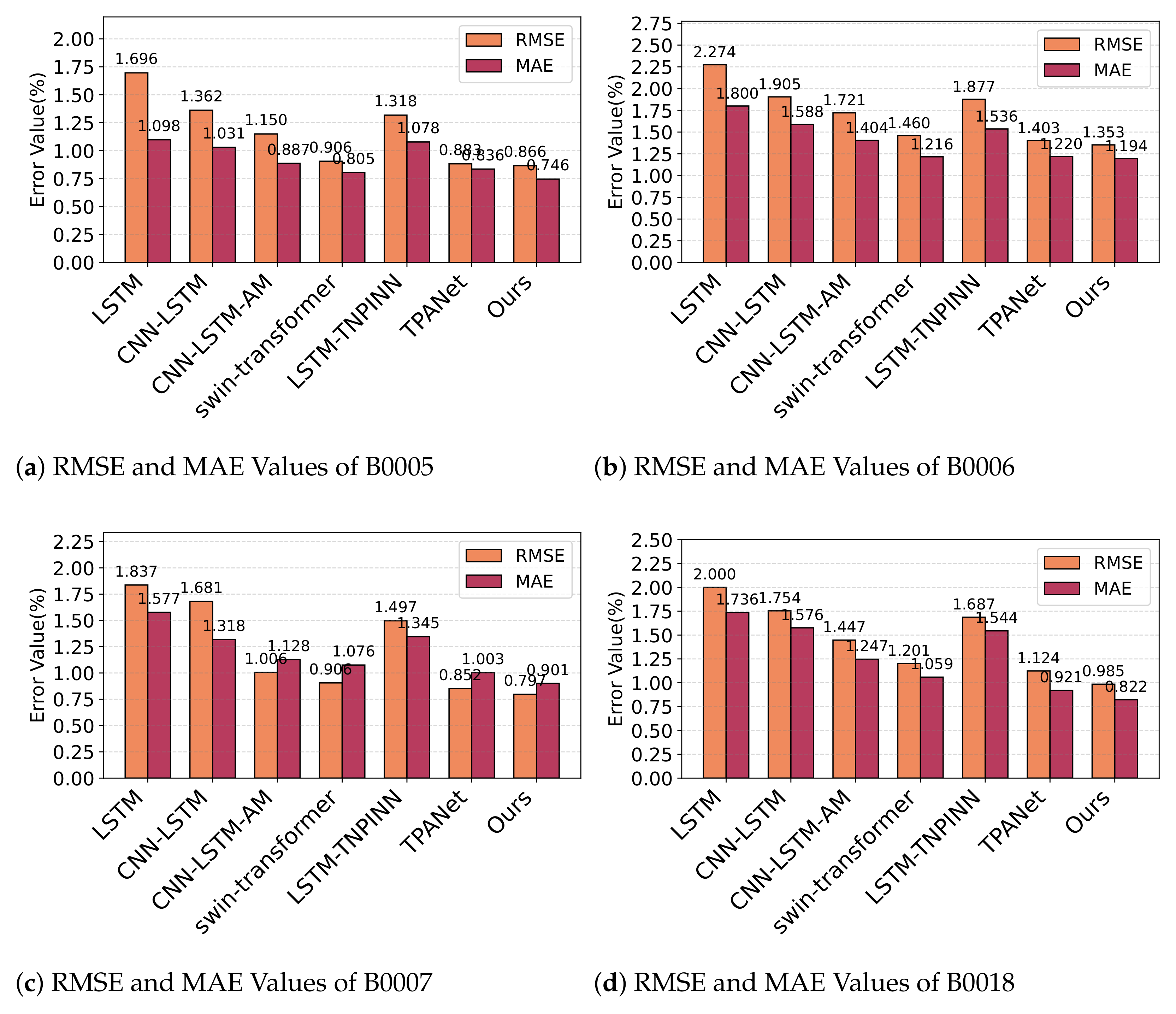
| B0005 | RMSE | 1.696 | 1.362 | 1.15 | 0.906 | 1.318 | 0.883 | 0.866 |
| MAE | 1.098 | 1.031 | 0.887 | 0.805 | 1.078 | 0.836 | 0.746 | |
| B0006 | RMSE | 2.274 | 1.905 | 1.721 | 1.46 | 1.877 | 1.403 | 1.353 |
| MAE | 1.8 | 1.588 | 1.404 | 1.216 | 1.536 | 1.22 | 1.194 | |
| B0007 | RMSE | 1.837 | 1.681 | 1.006 | 0.906 | 1.497 | 0.852 | 0.797 |
| MAE | 1.577 | 1.318 | 1.128 | 1.076 | 1.345 | 1.003 | 0.901 | |
| B0018 | RMSE | 2 | 1.754 | 1.447 | 1.201 | 1.687 | 1.124 | 0.985 |
| MAE | 1.736 | 1.576 | 1.247 | 1.059 | 1.544 | 0.921 | 0.822 |
| M1 | M2 | M3 | M4 | M5 | M6 | M7 | ||
|---|---|---|---|---|---|---|---|---|
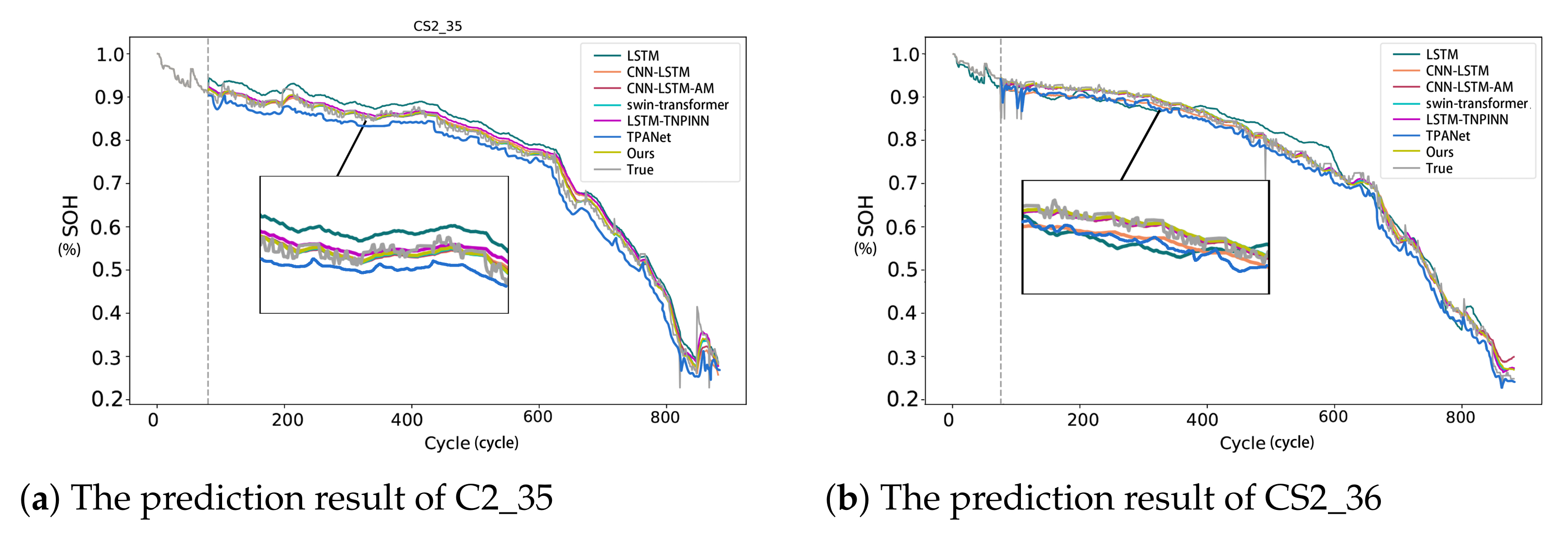
| CS2_35 | RMSE | 2.957 | 2.334 | 1.986 | 1.669 | 2.087 | 1.553 | 1.438 |
| MAE | 2.024 | 1.915 | 1.565 | 1.453 | 1.880 | 1.239 | 0.965 | |
| CS2_36 | RMSE | 3.016 | 2.85 | 1.586 | 1.49 | 2.768 | 1.386 | 1.324 |
| MAE | 2.085 | 1.827 | 1.366 | 1.24 | 1.726 | 1.115 | 1.097 | |
| CS2_37 | RMSE | 1.951 | 1.686 | 1.25 | 1.015 | 1.672 | 0.994 | 0.897 |
| MAE | 1.455 | 1.369 | 0.899 | 0.791 | 1.239 | 0.678 | 0.594 | |
| CS2_38 | RMSE | 2.303 | 1.719 | 1.594 | 1.282 | 1.706 | 1.137 | 0.964 |
| MAE | 1.497 | 1.301 | 0.964 | 0.869 | 1.206 | 0.804 | 0.7495 |
| Model | Metrics (%) | |||
|---|---|---|---|---|
| ✓ | ✓ | ✓ | ||
| ✗ | ✓ | ✓ | ||
| ✗ | ✗ | ✓ | ||
| B0005 | RMSE | 3.461 | 1.914 | 1.318 |
| MAE | 2.48 | 1.534 | 1.078 | |
| B0006 | RMSE | 3.266 | 2.648 | 1.877 |
| MAE | 3.015 | 2.224 | 1.536 | |
| B0007 | RMSE | 4.23 | 3.05 | 1.497 |
| MAE | 3.84 | 2.463 | 1.345 | |
| B0018 | RMSE | 3.436 | 2.735 | 1.687 |
| MAE | 2.821 | 2.23 | 1.544 |
| Model | Metrics (%) | |||
|---|---|---|---|---|
| ✓ | ✓ | ✓ | ||
| ✗ | ✓ | ✓ | ||
| ✗ | ✗ | ✓ | ||
| CS2_35 | RMSE | 3.678 | 2.744 | 2.087 |
| MAE | 3.794 | 2.467 | 1.880 | |
| CS2_36 | RMSE | 4.627 | 3.541 | 2.768 |
| MAE | 4.137 | 3.171 | 1.726 | |
| CS2_37 | RMSE | 3.671 | 2.947 | 1.672 |
| MAE | 3.4 | 2.489 | 1.239 | |
| CS2_38 | RMSE | 3.98 | 2.764 | 1.706 |
| MAE | 3.347 | 2.137 | 1.206 |
Disclaimer/Publisher’s Note: The statements, opinions and data contained in all publications are solely those of the individual author(s) and contributor(s) and not of MDPI and/or the editor(s). MDPI and/or the editor(s) disclaim responsibility for any injury to people or property resulting from any ideas, methods, instructions or products referred to in the content. |
© 2025 by the authors. Licensee MDPI, Basel, Switzerland. This article is an open access article distributed under the terms and conditions of the Creative Commons Attribution (CC BY) license (https://creativecommons.org/licenses/by/4.0/).
Share and Cite
Ding, Y.; Zhu, J.; Liu, Y.; Ning, D.; Qin, M. Integrated Framework of LSTM and Physical-Informed Neural Network for Lithium-Ion Battery Degradation Modeling and Prediction. AI 2025, 6, 149. https://doi.org/10.3390/ai6070149
Ding Y, Zhu J, Liu Y, Ning D, Qin M. Integrated Framework of LSTM and Physical-Informed Neural Network for Lithium-Ion Battery Degradation Modeling and Prediction. AI. 2025; 6(7):149. https://doi.org/10.3390/ai6070149
Chicago/Turabian StyleDing, Yan, Jinqi Zhu, Yang Liu, Dan Ning, and Mingyue Qin. 2025. "Integrated Framework of LSTM and Physical-Informed Neural Network for Lithium-Ion Battery Degradation Modeling and Prediction" AI 6, no. 7: 149. https://doi.org/10.3390/ai6070149
APA StyleDing, Y., Zhu, J., Liu, Y., Ning, D., & Qin, M. (2025). Integrated Framework of LSTM and Physical-Informed Neural Network for Lithium-Ion Battery Degradation Modeling and Prediction. AI, 6(7), 149. https://doi.org/10.3390/ai6070149