Enhancing Acoustic Leak Detection with Data Augmentation: Overcoming Background Noise Challenges

Abstract

A leak detection method is developed for leaks typically encountered in industrial production. Leaks of 1 mm diameter and less are considered at operating pressures up to 10 bar. The system uses two separate datasets—one for the leak noises and the other for the background noises—both are linked using a developed mixup technique and thus simulate leaks trained in background noises. A specific frequency window between 11 and 20 kHz is utilized to generate a quadratic input for image recognition. With this method, detection accuracies of over 95% with a false alarm rate under 2% can be achieved on a test dataset under the background noises of hydraulic machines in laboratory conditions.

1. Introduction

Industrial plant leaks pose serious safety and environmental risks, including the potential for explosions and the loss of hazardous substances [1,2]. In response, industries are moving from manual inspections to automated monitoring systems to mitigate these hazards, particularly in sectors like chemical, oil and gas, and power generation, which can be heavily impacted by gas leaks and fires [3]. Traditional detection methods, reliant on human senses and occasional use of devices such as thermal cameras or leak detectors, have demonstrated limitations [4]. Notably, leak detectors are constrained to point measurements, responding only after a significant gas volume has escaped near a detector and with a time delay in detection. In contrast, microphones are capable of monitoring larger volumes, offering a more effective solution for early detection. The advancement towards automated detection systems aims for prompt identification, categorization, and response to leaks, thereby enhancing employee and environmental safety [5]. Additionally, non-hazardous compressed air leaks lead to significant financial losses, estimated at 1.18 to 3.55 billion euros in Germany in 2019 [6]. The push for energy efficiency and the shift towards renewable energy sources underscore the importance of effective leak detection, especially for high-pressure hydrogen storage, highlighting both cost-saving and safety benefits [7]. Future leak detection systems may rely on sensor technology, such as microphones capable of detecting a wide frequency range, including ultrasonic signals. These sensors offer a cost-effective, weather-independent solution that surpasses traditional methods by detecting leaks in obscured or invisible areas [8,9]. A significant challenge remains: reliably distinguishing leak-specific acoustic signatures from the complex and variable background noise typically found in industrial environments. Furthermore, while supervised learning techniques are promising for classification [10,11,12,13], the optimal combination of signal pre-processing, feature extraction, and machine-learning models specifically tailored for the diverse sounds of industrial leaks is still an area of active research and requires further investigation to maximize accuracy and reliability.

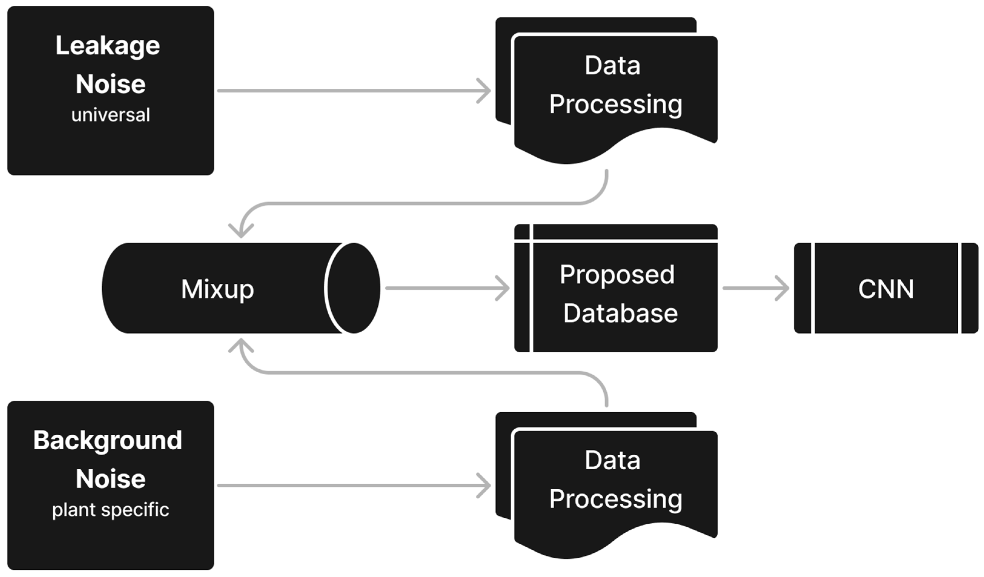
To achieve this objective, the methodology developed and evaluated in this study (Figure 1) utilizes microphone sensors capable of capturing a specific frequency range. The process involves collecting relevant acoustic data, which is then pre-processed using techniques potentially including band-pass filters [14,15] and appropriate frequency-time representations to enhance the Signal-to-Noise Ratio. Significant features are extracted, potentially using methods such as Short-Time Fourier Transformation (STFT) [16,17] to feed into specifically trained neural networks, particularly image-recognition-based models. A key aspect is the systematic linear combination (mixup) of laboratory leak measurements and plant-specific background noises to ensure the model’s robustness for supervised learning.

The following chapters outline the development and validation of this methodology in detail:

• Literature review with a focus on requirements for industrial use and a phenomenological description of leak noise and its effecting parameters as frequencies and sound levels
• Development of an appropriate procedure to train and validate an image-recognition model for leak detection based on laboratory leak measurements and background noises in industrial plants
• Data adjustment by means of a suitable frequency-time window
• Linear combination of laboratory leak measurements and plant-specific background noises
• Validation of the new methodology based on available literature data

2. Related Work

The main requirement for the leak detection system is a comprehensive monitoring capability across an entire industrial plant. To effectively monitor diverse industrial plants, a system must be both modular and scalable, accommodating different plant sizes and layouts. It would be desirable that the functionality does not depend on the hardware of the manufacturer. To assess this, a range of microphones from various manufacturers shall be tested, thereby evaluating their influence on the precision of detection, which has not yet been examined in this context. Furthermore, the system should not only provide a binary assessment (leak or no leak) but also a quantitative evaluation of the leak’s hazard potential. A small air leak requires a different intervention speed compared to a larger ammonia leak under the same pressure conditions. Through quantitative assessment, costly immediate interventions, such as dispatching to the leak site with potential plant shutdowns, should be avoided.

Additionally, the system should be able to differentiate between a leak and a planned pressure relief. Pressure reliefs and leaks share similar characteristics as they affect the sound field as both involve material discharge from the system. However, a pressure relief is intentionally conducted to control and lower the pressure level within a system. In contrast, a leak is an unplanned pressure relief, typically characterized by a significantly lower mass flow rate compared to a pressure release. The critical difference is that a planned pressure release is finite and terminates once the desired pressure level in the industrial process is achieved.

2.1. Phenomenological Description of Leak Noise Development

Leak dynamics, which include leak geometry and system pressure, can influence the detection accuracy of an acoustic leak detection system. In the chemical industry, production networks typically operate above pressures of 2 bar, and the dynamics of critical respectively choked flow become relevant. Leak dynamics are further affected by the ‘leak-before-break’ behavior in ductile piping material in chemical plants, where leaks or cracks form prior to a sudden complete rupture of a plant component [18,19]. This phenomenon shows that leaks are either stable or expand slowly, providing a crucial time window before catastrophic failure. The leak area is influenced by factors like crack length, geometry, material properties, and membrane tension [20]. Real-world leak geometries, often complex and irregular, are demonstrated by Silber et al. [21], who produced fatigue cracks and holes of various diameters. These geometries challenge the detection systems, as most literature overlooks specific leak contours, typically focusing on simplified models like circular leaks.

Chen et al. [22] explored critical flows behind rectangular nozzles, showing that the Aspect Ratio (AR) influences the fundamental frequency and affects the screech tones in critical flows [23]. These screech tones, resulting from interactions between flow instabilities and shock waves, are more pronounced with a reduced AR. This research underscores the significance of considering varying leak geometries and their impact on the sound spectrum, particularly in industrial settings where leaks may not be present as free jets due to closely spaced pipelines or valve environments.

Tam et al. [24] investigated experimental noise sources of free jets, concluding that fine-scale turbulence and large turbulence structures are the two primary noise sources. They found that fine-scale turbulence (St = 10²–10⁰) contributes to high-frequency noise due to small, rapidly changing eddies, while large turbulence structures generate low-frequency noise through larger, coordinated movements. Tam et al. [25] further examined the generation of screech tones in supercritical free jets, emphasizing the influence of nozzle geometry and flow dynamics on these tones. They identified these screech tones as a resonance phenomenon caused by interactions between large-scale flow structures and periodic shock waves within the jet, highlighting the critical role of large-scale coherent structures in producing these distinctive acoustic patterns.

CFD modeling for training data generation for machine learning is only suitable to a limited extent, as it requires a high computational effort since acoustic waves often have very small amplitudes and high frequencies, which means that the simulation must have very fine spatial and temporal resolution. To perform machine learning, enough training data is required, which is why many very time-consuming and energy-intensive modeling processes are necessary.

2.2. Measurement and Damping

Current considerations of monitoring systems include a network of stationary, interconnected sensors [26] and a rover equipped with microphones. While robot-based methods using IR sensors [8] and gas sensors [9] have been promising in laboratory settings, their practicality in industrial settings, with complex terrains and hazardous areas, remains limited [27,28].

Permanently installed sensors with continuous measurements, despite their higher cost due to the number required, offer detection of change in noises as a further parameter for comprehensive monitoring, particularly in hard-to-reach areas compared to mobile measurements. Future enhancements in communication technologies, such as 5G, could streamline data transmission and analysis [29], enhancing the effectiveness of stationary sensors in complex industrial environments compared to rover technology.

Kampelopoulos et al. [30] describe a method for detecting leaks in pipelines using accelerometer data and adaptive filtering to distinguish leak signals from background noise. By analyzing changes in energy levels across frequency bands, this method differentiates leaks from transient noise events. It relies on spectral analysis and percentage changes in root mean square (RMS) and slope sum features relative to a noise reference, enhancing accuracy in identifying leaks while minimizing false positives.

Besides one-phase flow, multiphase leak flows could be investigated for their influence on leak detection [31]. Real leak occurrences seldom match these models, highlighting the necessity of accounting for complex leak contours in detection efficacy.

Research by Abela et al. [32] shows that a 1 mm diameter air leak at 6 bar pressure produces 65 decibels, and a 1.5 mm leak up to 70 decibels. Previous studies from Santos et al. [33] and Da Cruz et al. [26] have focused on lower frequencies for internal pipe leak detection, overcoming challenges such as the need for drilling to install microphones. Li et al., Shibata et al., and Oh et al. have explored various leak sizes, distances, and frequencies [34,35,36]

2.3. Influence of Background Noise on Leak Detection

The training of machine-learning networks with real industrial noises on-site, despite being impractical, is crucial for effective detection and resilience to background noise in industrial environments. Background noise significantly affects the Signal-to-Noise Ratio (SNR), which is a key aspect in successfully implementing an acoustic leak detection system. A lower SNR means that background noise more easily masks leak signals. Oh et al. [36] suggest two main strategies: firstly, transforming acoustic signals using Fourier Transformation and analyzing patterns through autocovariance and autocorrelation; secondly, reducing data volume to filter out irrelevant information, thereby enhancing classification accuracy and efficiency. Particularly highlighted is the difficulty in distinguishing leaks from background noise, especially at full volume and when the Sound Pressure Level (SPL) of the leak is lower than the background noise. Additionally, Ning [37] developed a Spectrum-Enhancing (SE) method followed by Convolutional Neural Network (SE-CNN) processing. This involves applying STFT to the signal and extracting and amplifying the ultrasound range (20–40 kHz) while suppressing non-stationary signals. However, detection is limited within a 60° angle due to the characteristics of the used sound receiver directivity. Another approach is using CNNs to distinguish leak sounds from background noise. Johnson et al. [17] found that CNNs trained on leak sounds without background noise perform poorly in noisy environments, whereas those trained with background noises show improved accuracy. Data augmentation techniques like Random Erasing [38] or SpecAugment [39] further enhance detection in training without background noise.

However, these methods have not been tested in industry settings with authentic background noise. In real industrial environments characterized by louder and more varied background noises, these methods may be less effective, necessitating adaptations tailored to each specific setting. Training in more complex environments, particularly with varying microphone distances, significantly reduces detection accuracy. Despite testing in industrial settings, detection accuracy must approach 100% for practical implementation due to the high costs associated with false alarms and undetected leaks.

3. Materials and Methods

This chapter details the specific dataset utilized for training and testing the leak detection models, along with the methodologies employed for data structuring, processing, and augmentation. It further outlines the implementation of the proposed approach, the adaptation of neural network architectures, and the evaluation framework used to assess performance. The ProposedMethod—utilizing deep neural network architectures, frequency window selection (11–20 kHz applied to all data), and mixup data augmentation for training—is benchmarked against several alternatives. Firstly, it is compared to the NoNoise and OtherNoise approaches; these employ the same deep architecture and frequency window selection but differ by being trained without mixup augmentation, using training data consisting of leak recordings in laboratory background noise (NoNoise) and workshop background noise (OtherNoise), respectively. Secondly, a comparison is made with a reimplementation of Johnson et al.’s [17] shallower network architecture. This latter comparison was conducted without applying the frequency window selection and also without mixup augmentation, using training data prepared according to the NoNoise and OtherNoise procedures, specifically to isolate the combined benefits of the deep architectures, frequency windowing, and mixup data augmentation employed by the ProposedMethod.

3.1. Leak Dataset

The experimental work in this study is based on the publicly available IDMT-ISA-Compressed-Air (IICA) dataset [40] that comprises 5592 audio files, 32-bit resolution, and mono audio recorded in the frequency range of 3 Hz to 30 kHz. Two principal types of leaks were captured: tube and ventleaks, the latter of which was documented under two distinct system pressures to simulate varying operational conditions. This experimental setup aimed to ensure a comprehensive representation of potential leak scenarios.

The recording setup involved four Earthworks M30 microphones positioned at well-defined distances and angles relative to the leak source. This setup was designed to capture a broad spectrum of acoustic data:

• Microphone 1 was placed 20 cm from the leak point at a 90° angle, capturing the direct sound emission.
• Microphone 2 stood 2 m away, also at a 90° angle, to collect sound across a wider field.
• Microphone 3 was positioned 20 cm away but at a 30° angle, offering a different acoustic perspective.
• Microphone 4, located on the laboratory ceiling, was intended to record ambient acoustics, contrasting the near-field recordings from the other microphones.

The dataset simulation of operational conditions involves recordings through speakers under three distinct types of background noise to mimic real-world industrial environments: laboratory environment noise (Lab), workshop noise (Work), and hydraulic noise (Hydr). The laboratory environment contains minimal noise artefacts of the room itself. Hydraulic and workshop noises were played at both medium and loud volumes during recording sessions to further simulate varying operational conditions. This approach was designed to ensure the dataset’s applicability in training models for leak detection across a broad spectrum of real-world scenarios, enhancing its utility for practical applications in industrial settings. The pressure of the compressed air system is set to 6 bar with “tube” that should simulate a leaking tube. To limit bias in the data and obtain valid results, three recording sessions with the 15 configurations have been performed.

3.2. Data Structuring

While the foundational acoustic data is drawn from the publicly available IDMT-ISA-Compressed-Air (IICA) dataset [40], the core scientific contribution presented herein lies in the novel data structuring strategies and the specific methodologies derived and developed for processing, augmenting, and analyzing this data for robust leak detection. Figure 2 illustrates how the audio data is divided for training, validation, and testing of the leak detection model. Data from Microphones 1, 2, and 3, combined with different background noises (Lab, Workshop, or Hydraulic, representing various training conditions like ‘NoNoise’, ‘OtherNoise’, and ‘Benchmark’), is split into an 80% training dataset and a 20% validation dataset. Separately, data from Microphone 4, specifically combined with Hydraulic background noise, is used exclusively as the test dataset to evaluate the final classification performance (distinguishing ‘Leak’ from ‘No Leak’). A binary classification task was applied to the spectrograms, distinguishing between “no leak” (valve opening < 4.5 turns) and “leak present” (valve opening > 5.5 turns) based on the valve opening. Workshop noises were used for training and validation at both medium (m) and loud (l) volumes to further simulate varying operational conditions.

To evaluate the performance under different training conditions and establish comparative baselines, three distinct approaches developed for this study were implemented using the structured training data:

• NoNoise Method: Utilized recordings with laboratory background sound. This sound is assumed to be negligible due to the quiet laboratory environment; the spectrograms effectively contain only the leak noise.
• OtherNoise Method: Used recordings with workshop noise as the background sound.
• Benchmark Method: Employed recordings with hydraulic background sound, which is the same type of background noise used in the test dataset.

The test dataset is identical across all methods and consists of audio recordings from Microphone 4 with hydraulic background noises at both medium (m) and loud (l) volumes. The test dataset has an equal sample size as the validation dataset of all methods. To create a realistic simulation of industrial environments where the distance and angle from the leak to the microphone are unpredictable, microphone 4 is exclusively utilized —a microphone not included in the training data—as the test dataset. This deliberate choice enhances the authenticity of the detection process by accounting for the inherent variability in leak positions relative to the microphone, a common challenge in real-world operations. By testing the model with microphone 4, its ability to perform effectively under unfamiliar conditions is evaluated, ensuring that it can adapt to the uncertainties of distance and angle encountered in practical leak detection scenarios. This approach strengthens the model’s reliability and applicability in industrial settings where precise leak locations cannot be predetermined.

Table 1. Training, Validation, and Test datasets selection.

Method	Data Specification	Training/Validation Dataset		Test Dataset
All methods	Leak Status	Yes	No	Yes	No
	Knob Turns	6.0–9.0	0.0–4.0	6.0–9.0	0.0–4.0
	Microphone and Background Noise Volume	Microphone 1–3 (medium + loud)		Microphone 4 (medium + loud)
NoNoise	Background Noise	Lab		Hydr
OtherNoise	Background Noise	Work		Hydr
Benchmark	Background Noise	Hydr		Hydr

provides details on the audio recordings used for training in each method and for the test dataset.

The ProposedMethod—utilizing deep neural network architectures, frequency window selection, and mixup data augmentation for training—is benchmarked against several alternatives. Firstly, it is compared to the NoNoise and OtherNoise approaches; these employ the same deep architecture and frequency window selection but differ by being trained without mixup augmentation, using training data consisting of leak recordings in laboratory background noise (NoNoise) and workshop background noise (OtherNoise), respectively. Secondly, a comparison is made with a reimplementation of Johnson et al.’s [17] shallower network architecture. This latter comparison was conducted without applying the frequency window selection and also without mixup augmentation, using training data prepared according to the NoNoise and OtherNoise procedures, specifically to isolate the combined benefits of the deep architectures, frequency windowing, and mixup data augmentation employed by the ProposedMethod.

3.3. Proposed Method

The method is based on the idea that each facility has a model tailored to its location and operating conditions to adapt to the diversity of background noise. The variety of background noise in industrial environments, i.e., the frequency spectrum of machines, flow noises, and temporary activities in a certain installation of vessels and pipes, and the sound level differ largely from plant to plant. Minimum required training data based on the variety of plants are generally not available and cannot be simulated. Furthermore, in specific production environments, leaks are rather rare; they occur often less than once a year. Hence, the proposed method (ProposedMethod) is based on the concept of constructing two separate datasets from audio recordings. The first leak dataset is recorded in a lab setting without background noise and consists of a large variety of leak sounds at different sizes, upstream pressures, and leak geometries, which can be enlarged with new leak geometries and conditions. For the second dataset, industrial background noise has to be recorded on-site to capture the specific acoustic environment of the actual deployment location.

Both datasets are combined under parameter λ, determining the weighting of background and leak noise using the presented mixup technique (Figure 3).

The first leak dataset serves as the foundation for the model’s training regimen, ensuring a rich variety of leak signatures are available for analysis. A proposed dataset is then created by combining the first leak dataset with a second on-site recorded industrial background noise dataset (hydraulic background noise), employing a mixup technique. This crucial step involves the linear combination of spectrograms, a method that superposes leak sounds with on-site industrial noises to mirror the real acoustics of the industrial setting. This approach generates a training dataset that enables the CNN to effectively distinguish between leak and non-leak states without requiring the generation of real leaks in industrial environments.

3.4. Frequency Window Selection

Effective classification of acoustic leak signals amidst background noise requires careful selection of a frequency window. The primary goal is to target regions within the STFT spectrogram where the influence of disruptive background noise is minimized while the acoustic emissions characteristic of leaks are maximally preserved. This involves identifying a frequency band that optimizes the SNR, thereby enhancing detection accuracy. Furthermore, for practical deployment in industrial settings, the chosen frequency range must support adequate detection distances. This necessitates balancing the exclusion of low-frequency noise against the mitigation of atmospheric attenuation, which predominantly affects higher-frequency signals and can otherwise limit the system’s operational range. Based on these considerations, a frequency window of 11 kHz to 20 kHz is selected.

High-Pass-Filter: To establish the lower boundary of this window f_low, it is crucial to filter out prevalent low-frequency background noise common in industrial environments. Numerous sources contribute noise below 11 kHz, including air compressors generating mechanical and turbulent sounds (50 Hz–10 kHz) [41], specific bearing friction noises exhibiting peaks between 1.5 kHz and 7 kHz [42], and various industrial machines like pneumatic tools, grinders, saws, and textile equipment, which often share noise peaks around 10 kHz [43].

In contrast, the acoustic signatures of gas leaks, generated by turbulence as the gas escapes through small orifices, often occupy higher frequencies, extending well into the ultrasonic range. However, distinct screech tones were not consistently observed as dominant features within the analyzed frequency range in the spectrograms derived from the utilized dataset, especially for the leak orifices investigated. Potential reasons include the fundamental screech frequencies lying significantly above the analyzed range for small leaks, masking by the dominant broadband turbulent noise, or non-ideal conditions in the simulated leaks. Therefore, the primary acoustic feature targeted for leak detection in this work is the characteristic broadband turbulent noise.

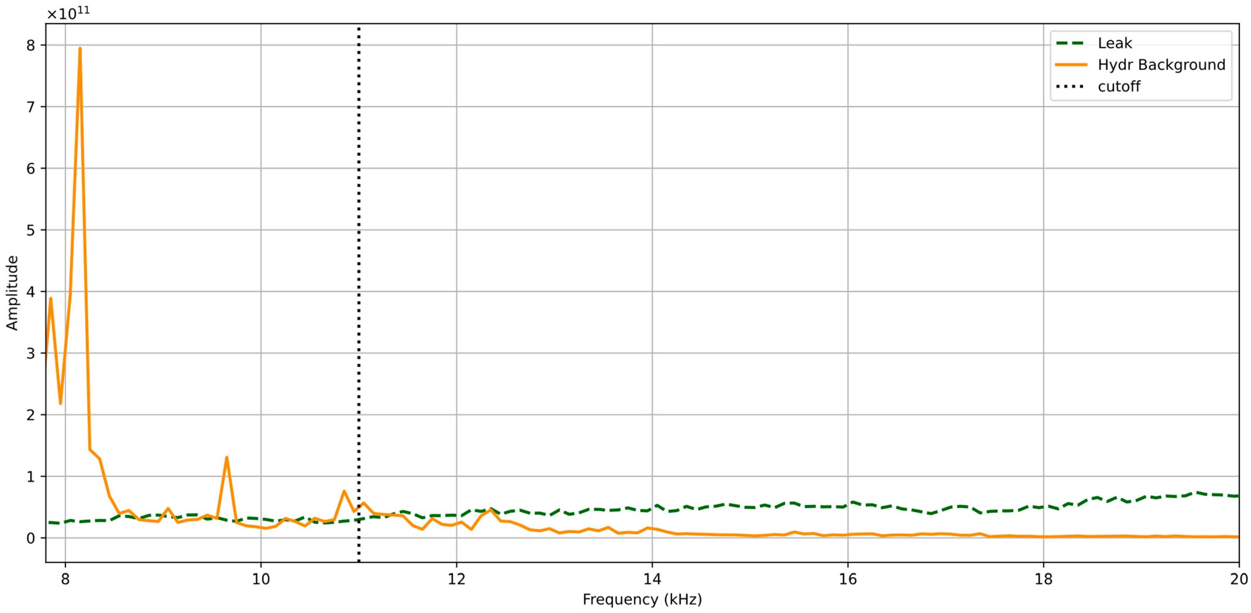
Previous research by Oh et al. [36] also supports this, demonstrating that a high-pass filter set at 10 kHz significantly improved SNR and leak detection rates. Visual analysis of the signal spectrograms, as represented in Figure 4, confirms this rationale. Figure 4 illustrates that while background noise energy is significant at lower frequencies, it decreases notably after its last peak, around 10.5 kHz. A vertical dashed line in the figure marks the selected cutoff at 11 kHz; this point is strategically chosen where the amplitude of typical leak noise consistently exceeds that of the background noise. Therefore, applying a high-pass filter with f_low = 11 kHz effectively attenuates substantial background noise while retaining the targeted higher-frequency leak signals.

Low-pass filter: Conversely, determining the upper boundary of the window (f_high) necessitates addressing the impact of air attenuation on signal propagation distance. Air attenuation is strongly frequency-dependent, increasing significantly at higher frequencies. For example, at 50% relative humidity and 20 °C, the attenuation rate climbs from 0.159 dB/m at 10 kHz to 1.661 dB/m at 50 kHz [44] (

Table 2. Sound propagation of leak noise sample calculated by inverse distance law for distance damping and ISO 9613-1:1993 [45] for air damping.

Frequency [kHz]	Distance [m]	Air Damping [dB, 50% Humidity, 20 °C]	Distance Damping 1/r [dB]	Total Damping [dB]
20	10	5.24	20	25.24
	25	13.1	27.96	41.06
30	10	9.36	20	29.36
	25	23.4	27.96	51.36

). This phenomenon severely dampens high-frequency components over distance, potentially limiting the effective range of the detection system. In many industrial scenarios, reliable detection is required over considerable distances, potentially up to 25 m or more, where total attenuation becomes substantial.

While the Strouhal calculations indicate leak frequencies can reach 20 kHz and beyond, frequencies significantly above 20 kHz suffer from rapidly increasing attenuation, making them less reliable for detection at a distance. Therefore, setting the upper cutoff frequency f_high to 20 kHz strikes a practical balance. It includes the primary frequency range identified for relevant leak sizes (up to 20 kHz based on the Strouhal example) while excluding higher frequencies where severe attenuation would drastically reduce the operational range. This low-pass filtering action mitigates the impact of excessive damping, ensuring more reliable performance across necessary detection distances within industrial facilities.

It is important to consider that the acoustic characteristics of a leak are not static nor solely defined by its initial orifice size. As a jet develops, its characteristic turbulent length scale increases with distance from the source; based on the Strouhal relation ($\mathrm{S}\mathrm{t}={\displaystyle \frac{\mathrm{f}\ast \mathrm{L}}{\mathrm{u}}}$, where L is the turbulent length scale). This increasing length scale implies that dominant frequencies (f) will shift towards lower values as the jet evolves downstream. Our Strouhal calculation—yielding a maximum jet diameter of approximately 3.3 mm covered by the 20 kHz upper band limit (assuming St = 0.2 and u = 330 ${\displaystyle \frac{\mathrm{m}}{\mathrm{s}}}$)—indicates that the chosen band effectively captures turbulent structures of this dimension, particularly near their origin. This assumption regarding the dynamic frequency evolution along the jet needs to be verified in future studies.

3.5. Implementation

The STFT is computed with a sampling rate f_s = 48,000 Hz, a window size N = 2048 samples, and a hop length H = 512 samples. These parameters define the frequency resolution of the spectrogram, as given by the following:

$$∆\mathrm{f}={\displaystyle \frac{{\mathrm{f}}_{\mathrm{s}}}{\mathrm{N}}}={\displaystyle \frac{\mathrm{48,000}}{2048}}~23.44 \mathrm{H}\mathrm{z}$$

(1)

Each frequency bin k in the STFT corresponds to a discrete frequency, calculated as:

$${\mathrm{f}}_{\mathrm{k}}=\mathrm{k}\cdot ∆\mathrm{f},\mathrm{k}=0,1,\dots .,{\displaystyle \frac{\mathrm{N}}{2}}=1024$$

(2)

To isolate the frequency range of 11–20 kHz, the bin indices k are identified such that $\mathrm{11,000} \le {\mathrm{f}}_{\mathrm{k}} \le \mathrm{20,000} \mathrm{H}\mathrm{z}$. The lower and upper bin indices are determined as follows:

• Lower bound:

$${\mathrm{k}}_{\mathrm{l}\mathrm{o}\mathrm{w}}=⌈{\displaystyle \frac{\mathrm{11,000} \mathrm{H}\mathrm{z}}{∆\mathrm{f}}}⌉=⌈{\displaystyle \frac{\mathrm{11,000}}{23.44}}⌉=⌈469.33⌉=470$$

(3)

• Upper bound:

$${\mathrm{k}}_{\mathrm{h}\mathrm{i}\mathrm{g}\mathrm{h}}=⌊{\displaystyle \frac{\mathrm{20,000} \mathrm{H}\mathrm{z}}{∆\mathrm{f}}}⌋=⌊{\displaystyle \frac{\mathrm{20,000}}{23.44}}⌋=⌊853.33⌋=853$$

(4)

Thus, the frequency range spans bins k = 470 to k = 853, corresponding to frequencies:

$${\mathrm{f}}_{470}=470\ast 23.44~\mathrm{11,015.63} \mathrm{H}\mathrm{z}, {\mathrm{f}}_{853}=853\ast 23.44~\mathrm{19,992.19} \mathrm{H}\mathrm{z}.$$

This effectively captures the desired 11–20 kHz band. The spectrogram is cropped by selecting from rows 470 to 853 of the STFT matrix. The number of frequency bins in the cropped spectrogram is:

$$\mathrm{N}\mathrm{u}\mathrm{m}\mathrm{b}\mathrm{e}\mathrm{r} \mathrm{o}\mathrm{f} \mathrm{b}\mathrm{i}\mathrm{n}\mathrm{s}=854-470=384$$

(5)

The resulting spectrogram matrix has 384 rows, each representing a frequency bin. The number of columns, or time frames T, depends on the signal length and hop size. For a signal chunk of 196,600 samples, T is calculated as:

$$\mathrm{T}=\left[{\displaystyle \frac{\mathrm{s}\mathrm{i}\mathrm{g}\mathrm{n}\mathrm{a}\mathrm{l} \mathrm{l}\mathrm{e}\mathrm{n}\mathrm{g}\mathrm{t}\mathrm{h}}{\mathrm{H}}}\right]=\left[{\displaystyle \frac{\mathrm{196,600}}{512}}\right]~384$$

(6)

After cropping, the absolute value of the STFT is taken, and the data is converted to a 32-bit floating-point format, yielding a final spectrogram matrix of size 384 × 384. This matrix encapsulates the magnitude information across 384 frequency bins and 384 timeframes, representing the 11–20 kHz frequency range of interest. Each mixed spectrogram is saved in a specified output directory. The file contains two arrays: a mixed spectrogram (expanded with an additional dimension for compatibility with the CNN input format) and a binary label indicating the presence or absence of a leak. Unlike some mixup implementations where labels are weighted based on the mixing coefficient (e.g., proportional to the contribution of each component in the training data), in this study, the labels are strictly binary and unaffected by the mixup process. This ensures a clear, binary classification approach without introducing weighted or intermediate label values. This implementation aims to enhance the diversity and representativeness of the augmented dataset, as the random shuffling of spectrogram pairs prevents bias in the mixing process. By applying the mixup technique directly to spectrograms rather than raw audio signals, the method aligns with the CNN’s input requirements, which operate on frequency–time representations, and reduces computational overhead by avoiding unnecessary transformations between time and frequency domains, preserving the spectral features critical for leak detection.

3.6. Data Augmentation with Mixup

To enhance the robustness and generalization of the CNN for leak detection, the mixup technique [46] is employed to augment the training dataset. This method involves linearly combining spectrograms from leak and background noise datasets to simulate realistic acoustic environments where leak signals are overlaid on industrial background noise.

The practical implementation of the mixup technique proceeds as follows: Spectrograms are sourced from two distinct directories—one containing leak spectrograms (leakfiledirectory) and the other containing background noise spectrograms (backgroundfiledirectory). These spectrograms represent the STFT of an audio signal. To maintain balance and randomness in the dataset, the lists of spectrogram files from both directories are shuffled independently using Python’s Fisher–Yates shuffle (version 3.10).

For each pair of spectrograms—one leak spectrogram and one background spectrogram—a mixed spectrogram is generated. The number of pairs is limited to the smaller of the two dataset sizes, ensuring equal representation from both classes. Let each spectrogram $\mathbf{S}\in {\mathbb{R}}^{\mathbf{M}\mathbf{\times }\mathbf{T}}$, where M represents the number of frequency bins, and T represents the number of time frames in the STFT. The mixed spectrogram is computed elementwise as follows:

$$S_{\mathrm{m}\mathrm{i}\mathrm{x}\mathrm{e}\mathrm{d}}\left[\mathrm{m},\mathrm{t}\right]=\mathsf{\lambda }\cdot {\mathrm{S}}_{\mathrm{l}\mathrm{e}\mathrm{a}\mathrm{k}}[\mathrm{m},\mathrm{t}]+(1-\mathsf{\lambda })\cdot {\mathrm{S}}_{\mathrm{b}\mathrm{a}\mathrm{c}\mathrm{k}\mathrm{g}\mathrm{r}\mathrm{o}\mathrm{u}\mathrm{n}\mathrm{d}}[\mathrm{m},\mathrm{t}]$$

(7)

For m = 1, 2, …, M and t= 1, 2, …, T, where S_leak and S_background are the STFTs of the leak and background noise signals, respectively. However, this linear combination overlooks the physical interference effects between sound waves, which involve both amplitude and phase interactions not captured in magnitude spectrograms alone. Acknowledging that even mixup in the complex STFT domain using independent recordings would face challenges in fully replicating spatially-dependent phase interactions of real-world acoustics, the computationally efficient approach of combining magnitude spectrograms was adopted for its direct applicability to practical data augmentation.

To optimize the mixup coefficient λ, it is evaluated that the similarity between the mixed spectrogram S_mixed and a reference spectrogram S_ref—defined here as the spectrogram of the leak signal in hydraulic background noise using Peak Signal-to-Noise Ratio (PSNR) and Pearson Correlation Coefficient. The purpose of comparing the generated S_mixed to the original S_ref is to find an optimal λ that ensures the mixed spectrogram realistically incorporates background noise while retaining sufficient fidelity and structural characteristics of the original leak signal for effective model training.

PSNR, which measures signal fidelity, is calculated as follows:

$$\mathrm{P}\mathrm{S}\mathrm{N}\mathrm{R}=20\cdot {\mathrm{l}\mathrm{o}\mathrm{g}}_{10}\left({\displaystyle \frac{{\mathrm{m}\mathrm{a}\mathrm{x}(\mathrm{S}}_{\mathrm{r}\mathrm{e}\mathrm{f}})}{\sqrt{\mathrm{M}\mathrm{S}\mathrm{E}}}}\right)$$

(8)

where max(S_ref) is the maximum intensity value in the reference spectrogram. The mean squared error (MSE) between the matrices of S_mixed and S_ref is as follows:

$$\mathrm{M}\mathrm{S}\mathrm{E}={\displaystyle \frac{1}{384\times 384}}\sum _{\mathrm{i}=1}^{384}\sum _{\mathrm{j}=1}^{384}{({\mathrm{S}}_{\mathrm{m}\mathrm{i}\mathrm{x}\mathrm{e}\mathrm{d}}\left[\mathrm{i},\mathrm{j}\right]-{\mathrm{S}}_{\mathrm{r}\mathrm{e}\mathrm{f}}\left[\mathrm{i},\mathrm{j}\right])}^2$$

(9)

This quantifies the average squared difference in amplitude across all frequency bins and time frames.

The Pearson Correlation Coefficient, assessing linear similarity, is computed from the flattened intensity values of both spectrograms as follows:

$$\mathrm{r}={\displaystyle \frac{{\sum }_{\mathrm{k}=1}^{{384}^2}({\mathrm{S}}_{\mathrm{m}\mathrm{i}\mathrm{x}\mathrm{e}\mathrm{d}}-{\overline{\mathrm{S}}}_{\mathrm{m}\mathrm{i}\mathrm{x}\mathrm{e}\mathrm{d}})({\mathrm{S}}_{\mathrm{r}\mathrm{e}\mathrm{f},\mathrm{k}}-{\overline{\mathrm{S}}}_{\mathrm{r}\mathrm{e}\mathrm{f}})}{\sqrt{{\sum }_{\mathrm{k}=1}^{{384}^2}({{\mathrm{S}}_{\mathrm{m}\mathrm{i}\mathrm{x}\mathrm{e}\mathrm{d}}-{\overline{\mathrm{S}}}_{\mathrm{m}\mathrm{i}\mathrm{x}\mathrm{e}\mathrm{d}})}^2{\sum }_{\mathrm{k}=1}^{{384}^2}{({\mathrm{S}}_{\mathrm{r}\mathrm{e}\mathrm{f},\mathrm{k}}-{\overline{\mathrm{S}}}_{\mathrm{r}\mathrm{e}\mathrm{f}})}^2}}}$$

(10)

Here, S_mixed,k and S_ref,k are the intensity values at position k in the flattened arrays (with k ranging from 1 to 384²), and ${\overline{\mathrm{S}}}_{\mathrm{m}\mathrm{i}\mathrm{x}\mathrm{e}\mathrm{d}}$ and ${\overline{\mathrm{S}}}_{\mathrm{r}\mathrm{e}\mathrm{f}}$ are the mean intensities of the respective spectrograms. This metric captures the structural alignment between the two spectrograms.

Since the mixup process uses magnitude spectrograms, both PSNR and Pearson correlation focus on amplitude differences, ignoring phase interactions. Testing λ from 0.1 to 0.9, the optimal balance is found at 0.5 (Figure 5), a high PSNR for preserved signal quality, and a moderate Pearson correlation to avoid overfitting, enhancing the CNN’s generalization for leak detection in noisy conditions.

3.7. Adjustment of Network Architectures

In this study, three CNN architectures are adapted—AlexNet, ResNet18, and VGG16—to process a dataset of 384 × 384 grayscale images for a binary classification task. Originally designed for 224 × 224 RGB images and multi-class classification, these networks required specific modifications to accommodate the data’s single-channel input, higher resolution, and binary output requirements. Below, the general modifications applied across all three networks are outlined, and a detailed example of the changes made to AlexNet, including its modified architecture table, is provided. Similar adjustments were made to ResNet18 and VGG16, with their detailed architectures provided in

Table A2. Adjusted(A)-ResNet18 architecture for the (384, 384) grayscale input. * For Layers 4, 5, and 6, the stride of 2 applies only to the first BasicBlock in each pair; the second has stride 1.

Layer	Type	Filters	Kernel	Stride	Padding	Output Dimension	Parameters
1	Conv2D	64	3 × 3	1	1	(64, 384, 384)	576
2	BatchNorm2d	-	-	-	-	(64, 384, 384)	128
3	BasicBlock ×2	64	3 × 3	1	1	(64, 384, 384)	147,968
4	BasicBlock ×2	128	3 × 3	2 *	1	(128, 192, 192)	525,568
5	BasicBlock ×2	256	3 × 3	2 *	1	(256, 96, 96)	2,099,712
6	BasicBlock ×2	512	3 × 3	2 *	1	(512, 48, 48)	8,393,728
7	AvgPool2D	-	4 × 4	4	0	(512, 12, 12)	0
8	Linear	-	-	-	-	1	73,729

and

Table A3. Adjusted(A)-VGG16 architecture for the (384, 384) grayscale input.

Layer	Type	Filters	Kernel	Stride	Padding	Output Dimension	Parameters
1	Conv2D	64	3 × 3	1	1	(64, 384, 384)	640
2	Conv2D	64	3 × 3	1	1	(64, 384, 384)	36,928
3	MaxPool2D	-	2 × 2	2	0	(64, 192, 192)	0
4	Conv2D	128	3 × 3	1	1	(128, 192, 192)	73,856
5	Conv2D	128	3 × 3	1	1	(128, 192, 192)	147,584
6	MaxPool2D	-	2 × 2	2	0	(128, 96, 96)	0
7	Conv2D	256	3 × 3	1	1	(256, 96, 96)	295,168
8	Conv2D	256	3 × 3	1	1	(256, 96, 96)	590,080
9	Conv2D	256	3 × 3	1	1	(256, 96, 96)	590,080
10	MaxPool2D	-	2 × 2	2	0	(256, 48, 48)	0
11	Conv2D	512	3 × 3	1	1	(512, 48, 48)	1,180,160
12	Conv2D	512	3 × 3	1	1	(512, 48, 48)	2,359,808
13	Conv2D	512	3 × 3	1	1	(512, 48, 48)	2,359,808
14	MaxPool2D	-	2 × 2	2	0	(512, 24, 24)	0
15	Conv2D	512	3 × 3	1	1	(512, 24, 24)	2,359,808
16	Conv2D	512	3 × 3	1	1	(512, 24, 24)	2,359,808
17	Conv2D	512	3 × 3	1	1	(512, 24, 24)	2,359,808
18	MaxPool2D	-	2 × 2	2	0	(512, 12, 12)	0
19	Linear	-	-	-	-	4096	301,993,384
20	Linear	-	-	-	-	4096	16,781,312
21	Linear	-	-	-	-	1	4097

. The following adaptations were consistently applied to all three networks:

• Input Channel Adjustment: The original architectures were designed for three-channel RGB inputs. To process the single-channel grayscale images, the first convolutional layer in each network is modified to accept one input channel instead of three. This adjustment ensures compatibility with the dataset while maintaining the integrity of the subsequent layers.
• Handling Larger Input Size: To leverage the increased resolution of the 384 × 384 images, the networks are adjusted to handle the larger feature maps produced by the convolutional layers. For AlexNet and VGG16, this required recalculating and updating the input size of the first fully connected layer to match the expanded spatial dimensions of the feature maps (e.g., from 256 × 6 × 6 to 256 × 11 × 11 for AlexNet and from 512 × 7 × 7 to 512 × 12 × 12 for VGG16). For ResNet18, which uses average pooling with a fixed kernel size of 4, the feature map size after pooling changes with the input size, necessitating an adjustment to the input size of the final linear layer (e.g., to 73,728 features for 384 × 384 inputs).
• Output Layer Configuration: Designed for multi-class classification (e.g., 1000 classes for ImageNet), the original output layers were replaced with a single neuron followed by a sigmoid activation function to produce a probability score for the binary classification task. This modification aligns the networks’ outputs with the detection objectives.

These changes enabled the networks to process grayscale images, capture finer details from the higher-resolution inputs, and perform binary classification effectively. The convolutional layers themselves remained largely unchanged, as they can naturally adapt to different input sizes, with adjustments confined primarily to the input and fully connected layers. An illustrative example is made in Appendix A.

3.8. Normalization

The input STFT spectrograms are normalized using Z-score normalization to mitigate the effect of differing scales and distributions, leading to improved model convergence and performance.

Z-Score normalization is applied as Equation (11) as follows:

$$S_{\mathrm{n}\mathrm{o}\mathrm{r}\mathrm{m}}\left[\mathrm{m},\mathrm{t}\right]={\displaystyle \frac{\mathrm{S}[\mathrm{m},\mathrm{t}]-\mathsf{\mu }}{\sigma +\mathsf{\epsilon }}}$$

(11)

With:

$$\mathsf{\mu }={\displaystyle \frac{1}{\mathrm{M}\mathrm{T}}}\sum _{\mathrm{m}=1}^{\mathrm{M}}\sum _{\mathrm{t}=1}^{\mathrm{T}}\mathrm{S}[\mathrm{m},\mathrm{t}]$$

(12)

Is the mean of all elements in the spectrogram,

$$\sigma =\sqrt{{\displaystyle \frac{1}{\mathrm{M}\mathrm{T}}}\sum _{\mathrm{m}=1}^{\mathrm{M}}\sum _{\mathrm{t}=1}^{\mathrm{T}}{(\mathrm{S}\left[\mathrm{m},\mathrm{t}\right]-\mathsf{\mu })}^2}$$

(13)

$\sigma$ is the standard deviation of all elements in the spectrogram, and $\mathsf{\epsilon }=1\times {10}^{-10}$ is a small constant added to the standard deviation to prevent division by zero. This normalization ensures that each spectrogram has a mean of zero and a standard deviation of one, providing consistent scaling across all input samples for effective neural network training.

3.9. Evaluation Metrics

Three widely accepted metrics are employed to assess the performance of the CNN for binary classification: accuracy, precision, and recall. These metrics collectively provide a robust evaluation of the model’s predictive capability.

The metrics are calculated based on the confusion matrix elements for a given test set:

• Accuracy: Measures the overall proportion of correct predictions:

$$\mathrm{A}\mathrm{c}\mathrm{c}\mathrm{u}\mathrm{r}\mathrm{a}\mathrm{c}\mathrm{y}={\displaystyle \frac{\mathrm{T}\mathrm{P}+\mathrm{T}\mathrm{N}}{\mathrm{T}\mathrm{P}+\mathrm{T}\mathrm{N}+\mathrm{F}\mathrm{P}+\mathrm{F}\mathrm{N}}}$$

(14)

• Precision: Quantifies the correctness of positive predictions

$$\mathrm{P}\mathrm{r}\mathrm{e}\mathrm{c}\mathrm{i}\mathrm{s}\mathrm{i}\mathrm{o}\mathrm{n}={\displaystyle \frac{\mathrm{T}\mathrm{P}}{\mathrm{T}\mathrm{P}+\mathrm{F}\mathrm{P}}}$$

(15)

• Recall: Assesses the model’s ability to identify all actual positives

$$\mathrm{R}\mathrm{e}\mathrm{c}\mathrm{a}\mathrm{l}\mathrm{l}={\displaystyle \frac{\mathrm{T}\mathrm{P}}{\mathrm{T}\mathrm{P}+\mathrm{F}\mathrm{N}}}$$

(16)

where:

• TP: True Positives (leaks correctly predicted)
• TN: True Negatives (non-leaks correctly predicted)
• FP: False Positives (non-leaks incorrectly predicted)
• FN: False Negatives (leaks incorrectly predicted)

These definitions ensure a precise mathematical foundation for evaluating CNN’s performance.

To mitigate the impact of randomness in the training process—such as random weight initialization and data shuffling—each experimental configuration of the CNN is trained and evaluated five times. This multi-run strategy enhances the reliability of the results by capturing variability across independent runs, ensuring that reported metrics reflect consistent model behavior rather than a single, potentially anomalous outcome.

For each of the five runs, the test set values of accuracy, precision, and recall are computed after training.

Section 4 reports the mean values of accuracy, precision, and recall, accompanied by their standard deviations, providing a clear summary of both average performance and consistency. To enhance interpretability, graphs include error bars corresponding to the standard deviation for each metric. These error bars visually convey the variability across the five runs, offering an intuitive representation of the model’s stability alongside its central tendency. Metrics are calculated during the test phase of each run using torchmetrics, ensuring accurate aggregation of the test set. After completing each run, the metric values are exported to Tables, where the mean and standard deviation are computed. This process guarantees both precision in metric calculation and transparency in statistical analysis.

3.10. Experimental Setup

For calculation, a high-performance computing configuration comprising an HP ML350 G9 Server equipped with an Intel Xeon E5 Processor and 128 GB of RAM, alongside an Nvidia Tesla Ampere A100 40GB GPU, is used. This hardware selection was aimed at leveraging GPU’s computational power to efficiently handle the extensive requirements of a spatial spectrogram input and the training of sophisticated neural network models in PyTorch 2.4.0 and CUDA 12.1. The dataloader setup utilizes a CustomDataset class to load and normalize spectrogram data, incorporating validation checks to ensure only clean, standardized inputs are processed. For the training set, the DataLoader shuffles the data at each epoch to randomize sample order, promoting better model generalization. Meanwhile, the validation and test sets are kept unshuffled to maintain a consistent order, ensuring reliable evaluation and preserving sequence integrity for accurate real-world performance assessment.

This partitioning strategy ensures enough data for training while also reserving a representative subset for model validation.

4. Results

Section 4.1 provides a comparative analysis of four detection methods—NoNoise, OtherNoise, Benchmark, and ProposedMethod—implemented with an adapted ResNet18 architecture for audio leak detection, focusing on tubeleaks and ventleaks under different noise conditions. Section 4.2 examines how different neural network architectures, such as the deeper (A)-ResNet18, (A)-VGG16, and (A)-AlexNet, compare to the shallower 3CONV3POOL network in detecting tubeleaks and ventleaks under varying noise conditions and training approaches. It investigates the impact of network depth and the role of background noise during training, revealing unique challenges and performance differences between the two leak types. Section 4.3 provides a comparative analysis of detection accuracies for tubeleak and ventleak scenarios, pitting the ProposedMethod—utilizing (A)-ResNet18 for tubeleak and (A)-VGG16 for ventleak—against Johnson et al.’s method, which relies on a smaller input format. Lastly, Section 4.4 compares how well the (A)-ResNet18 architecture detects tubeleaks and (A)-VGG16 detects ventleaks using three methods—OtherNoise, Benchmark, and ProposedMethod—by analyzing precision and recall, which measure false alarm rates and the ability to catch all real leaks, respectively. It highlights the trade-offs each method faces in balancing reliable detection with minimizing errors, especially in noisy settings, paving the way for future improvements.

4.1. Comparison of Methods

Figure 6 compares the detection accuracies of four methods implemented using an adapted ResNet18 architecture with the (384, 384) input: NoNoise (training with lab background noise), OtherNoise (training with work background noises and testing on hydraulic background noises), Benchmark (training with the same hydraulic background noises as in testing), and the ProposedMethod (the novel approach). Across all methods, ventleak detection consistently outperforms tubeleak detection. The ProposedMethod achieves accuracies of 92.4% for ventleaks and 86.4% for tubeleaks, significantly surpassing OtherNoise (82.5% for ventleaks, 62.9% for tubeleaks) and closely approaching the Benchmark (93.2% for ventleaks, 88.7% for tubeleaks). Training without background noise (NoNoise) yields inadequate results—53.8% for ventleaks and 45.7% for tubeleaks—marked with an asterisk due to its impracticality.

Notably, OtherNoise exhibits the largest spread in accuracy, with a 19.6 percentage point difference between ventleaks and tubeleaks, compared to a 6.0 percentage point spread for the ProposedMethod. While achieving a mean accuracy slightly below the Benchmark, these results underscore the ProposedMethod’s highly competitive and reliable performance, especially relative to NoNoise and OtherNoise.

4.2. Influence of Network Architecture on Detection Accuracy for Tubeleaks and Ventleaks

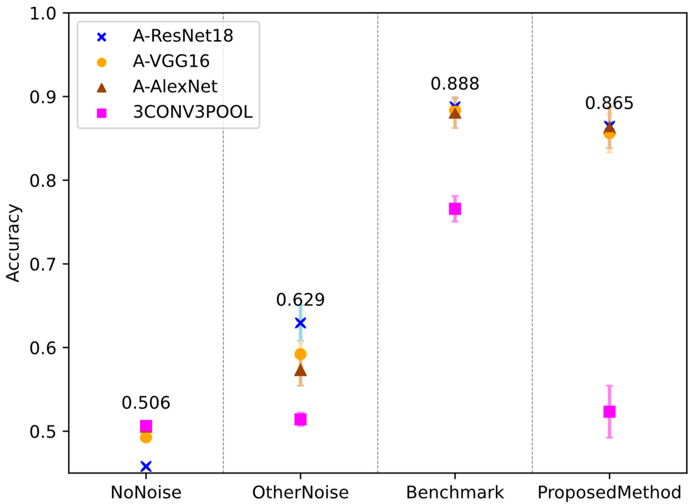
Figure 7 demonstrates that deeper networks—(A)-ResNet18, (A)-VGG16, and (A)-AlexNet—consistently outperform the shallower 3CONV3POOL network for tubeleaks across OtherNoise, Benchmark, and ProposedMethod.

These networks achieve accuracies of 0.85–0.88 with the ProposedMethod and 0.88 with the Benchmark, with (A)-ResNet18 reaching 86.5% and 88.8%, respectively (

Table 3. Accuracy values for different methods on network architectures for the (384, 384) input for tubeleaks.

Metrik	Method	(A)- VGG16	(A)- ResNet18	(A)- AlexNet	3CONV 3POOL
Accuracy	Benchmark	0.884	0.888	0.881	0.766
	Proposed	0.856	0.865	0.863	0.523
	NoNoise	0.493	0.458	0.505	0.506
	OtherNoise	0.592	0.629	0.573	0.514

).

In contrast, 3CONV3POOL, comprising three convolutional and three pooling layers followed by linear layers with 884,832 parameters (see

Table A4. 3CONV3POOL architecture for the (384, 384) grayscale input.

Layer	Type	Filters	Kernel	Stride	Padding	Output Dimension	Parameters
1	Conv2D	6	3 × 3	1	1	(6, 384, 384)	60
2	MaxPool2D	-	2 × 2	2	0	(6, 192, 192)	0
3	Conv2D	12	3 × 3	1	1	(12, 192, 192)	660
4	MaxPool2D	-	2 × 2	2	0	(6, 96, 96)	0
5	Conv2D	24	3 × 3	1	1	(24, 96, 96)	2616
6	MaxPool2D	-	2 × 2	2	0	(24, 48, 48)	0
7	Linear	-	-	-	-	96	5,308,704
8	Linear	-	-	-	-	1	97

), falls to 52.3% for ProposedMethod—a gap of over 30%. This underperformance may stem from its limited depth, hindering complex feature extraction compared to deeper architectures with residual or extensive convolutional stacks. Training without background noise (NoNoise) yields poor results across all networks, with accuracies around 0.5, barely above random guessing, underscoring background noise’s critical role in the training process.

Shifting to ventleaks, Figure 8 reveals (A)-AlexNet as the top performer for the Benchmark, achieving 0.971 accuracy, and (A)-VGG16 as top performer at 0.960 with the ProposedMethod, compared to 3CONV3POOL’s 0.944 at Benchmark and 0.889 at ProposedMethod (

Table 4. Accuracy values for different methods and network architectures for the (384, 384) input for ventleaks.

Metrik	Method	(A)- VGG16	(A)- ResNet18	(A)- AlexNet	3CONV 3POOL
Accuracy	Benchmark	0.968	0.932	0.971	0.944
	Proposed	0.960	0.924	0.940	0.889
	NoNoise	0.628	0.539	0.562	0.608
	OtherNoise	0.920	0.825	0.900	0.710

).

Deeper networks generally excel, with (A)-AlexNet peaking at 0.971 under Benchmark—far exceeding tubeleaks’ 0.884 in the same condition—indicating task-specific resilience. Nevertheless, 3CONV3POOL remains the weakest, though its ventleak accuracies (e.g., 0.889 under ProposedMethod) surpass its tubeleak results (52.3%), suggesting some adaptability. The higher OtherNoise performance by nearly 30% for ventleaks contrasts with tubeleaks, highlighting distinct detection challenges. Practical challenges due to different leak geometries in training and testing come up and must be solved in future investigations.

4.3. Comparison of the Proposed Method Against a Literature Method

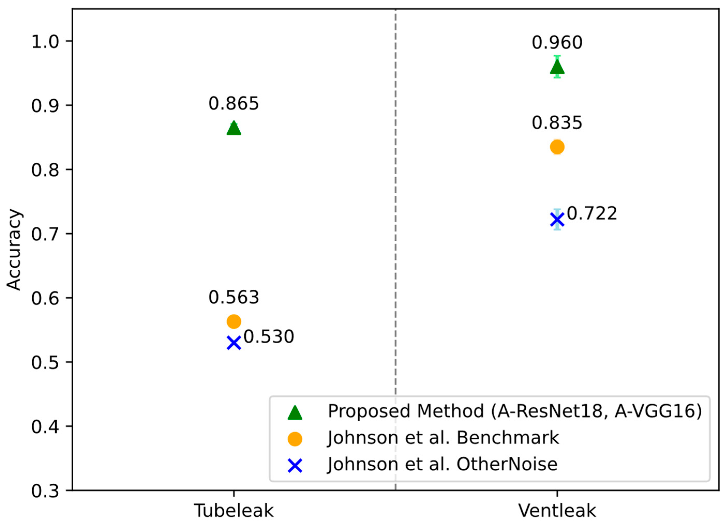
Figure 9 compares the detection accuracy of the ProposedMethod—using (A)-ResNet18 for tubeleak and (A)-VGG16 for ventleak—against the method by Johnson et al. [17], which employs a (1025, 24) input format (

Table A5. Rebuilt architecture from Johnson et al. [17] for the (1024, 24) grayscale input.

Layer	Type	Filters	Kernel	Stride	Padding	Output Dimension	Parameters
1	Conv2D	6	3 × 3	1	1	(6, 1024, 24)	60
2	MaxPool2D	-	2 × 2	2	0	(6, 512, 12)	0
3	Dropout	-	-	-	-	(6, 512, 12)	0
4	Conv2D	12	3 × 3	1	1	(12, 512, 12)	660
5	MaxPool2D	-	2 × 2	2	0	(12, 256, 6)	0
6	Dropout	-	-	-	-	(12, 256, 6)	0
7	Conv2D	24	3 × 3	1	1	(24, 256, 6)	2616
8	MaxPool2D	-	2 × 2	2	0	(24, 128, 3)	0
9	Linear	-	-	-	-	96	884,832
10	Dropout	-	-	-	-	96	0
11	Linear	-	-	-	-	1	97

). The graph, divided into tubeleak (left) and ventleak (right) sections, uses green triangles for the ProposedMethod with (A)-ResNet18 (left) and (A)-VGG16 (right), yellow dots for Johnson et al.’s architecture with Benchmark, and blue ‘X’s for Johnson et al.’s architecture with OtherNoise.

For tubeleak detection, the ProposedMethod achieves 86.4% accuracy, significantly outperforming Johnson et al.’s Benchmark at 56.3% and Johnson et al.’s OtherNoise at 53.0%, as indicated by the green triangles towering over the yellow dots and blue ‘X’s. This represents an improvement of over 30% compared to both methods. For ventleak detection, the ProposedMethod reaches 96.0%, surpassing the Benchmark’s 83.5% and OtherNoise’s 72.2%—a gain exceeding 20%. Across all methods, ventleak detection consistently outperforms tubeleak detection, a trend evident in the higher accuracies on the graph’s right side.

The ProposedMethod’s superior performance likely stems from two key factors: the deeper architectures of (A)-ResNet18 and (A)-VGG16, which enhance feature extraction compared to Johnson et al.’s method with its smaller (1025, 24) input, and the strategic selection of a specific frequency window. This frequency filtering minimizes the impact of background noise while preserving stationary information, which is critical since leak signals can be considered quasi-stationary. By isolating relevant frequency bands, the method effectively distinguishes leak signals from noise, further improving detection accuracy.

4.4. Precision and Recall Analysis for Tube and Vent Leaks

Figure 10 presents the precision and recall for detecting tube and ventleaks using the (A)-ResNet18 architecture across three methods: OtherNoise (training with varied noise), Benchmark (the standard approach), and ProposedMethod (the novel approach). Precision, which measures the false alarm rate (non-leaks incorrectly identified as leaks), is exceptionally high. It is important to note that these specific precision and recall figures depend on the classification threshold used; adjusting this threshold allows trading off higher precision for lower recall or vice versa. For ventleaks, all methods achieve near-perfect precision, reaching 100% in Benchmark and ProposedMethod (yellow ‘X’s), meaning no false positives. For tubeleaks, precision is 100% in OtherNoise and Benchmark, dropping slightly to 98.9% in ProposedMethod (yellow ‘X’s), still exceeding 98%, as shown in Figure 8.

Recall, which indicates the proportion of actual leaks detected (or conversely, the rate of undetected leaks), is lower across all methods. For tubeleaks, recall ranges from a low of 0.325 in OtherNoise (green ‘X’s) to 0.792 in Benchmark, settling at 0.758 in ProposedMethod. For ventleaks, recall improves from 0.676 in OtherNoise to 0.874 in Benchmark and 0.859 in ProposedMethod (green circles). This indicates a higher rate of undetected leaks, particularly for tubeleaks trained with varied background noise (OtherNoise), where recall drops to 0.325—significantly lower than the 0.792 achieved in Benchmark. High precision ensures minimal false alarms, which are vital for practical applications, while lower recall, especially in noisy conditions, suggests a challenge in detecting all leaks that warrant further optimization.

5. Discussion

The results of this study highlight the effectiveness of the ProposedMethod in addressing the challenge of binary detection of compressed air leaks at 6 bar pressure, two different leak geometries, particularly under varying speaker-induced background noise conditions. The findings build on previous research, such as [17], which emphasized the difficulty of detecting leaks under different background noise conditions.

By training a mixed leak and background dataset, the ProposedMethod achieves detection accuracies approaching those of the Benchmark for tubeleaks and ventleaks. Despite the simplification inherent in the mixup method, which neglects interference effects by employing a linear combination of leak and background signals, this approach significantly enhances the model’s generalization capability in noisy environments. This improvement is evidenced by its superior detection accuracy compared to models trained either without background noise or with alternative noise profiles. These findings suggest that the linear mixing strategy effectively simulates a diverse array of noise conditions, thereby enhancing the model’s robustness.

A key observation from the results is the influence of network architecture on detection performance. Deeper architectures, including (A)-AlexNet, (A)-VGG16, and (A)-ResNet18, consistently outperformed shallower models, particularly for tubeleaks. This aligns with findings from Section 4.2, which suggest that deeper networks excel at capturing complex features in noisy data. The improved performance for tubeleaks may stem from the networks’ ability to model intricate acoustic patterns obscured by leak noises. In contrast, ventleaks exhibited high detection accuracy across all architectures, likely due to their more distinct frequency signatures. This difference underscores the role of leak geometry in detection success and suggests that practical deployment might require either geometry-specific model tuning or the development of robust features across a wider variety of leak types. This aspect requires further investigation using a broader range of realistic leak geometries.

The ProposedMethod, using (A)-ResNet18 for tubeleak detection and (A)-VGG16 for ventleak detection, outperformed Johnson et al.’s [17] network architecture using the Benchmark and the OtherNoise method for both tubeleaks and ventleaks. This improvement can be attributed to the method’s enhanced feature extraction in the frequency domain, which better discriminates leak signals from noise compared to traditional approaches. Furthermore, deeper network architectures enhance the capability to detect complex leak patterns. Notably, the (A)-ResNet18 architecture achieved 100% precision for ventleaks across the OtherNoise, Benchmark, and ProposedMethod scenarios. This high precision indicates a low false-positive rate, a critical advantage in industrial applications where false alarms can trigger unnecessary facility shutdowns or dispatches. However, achieving such perfect precision, even on a test set with variations in noise and microphone placement, warrants careful consideration regarding potential overfitting to the specific characteristics of the IICA dataset. While encouraging, this result emphasizes the critical need for validation on entirely independent data, preferably captured in diverse real-world industrial environments, to definitively assess the model’s generalization capabilities and confirm its robustness against unseen conditions.

6. Conclusions

The significance of the method lies in the ability to reliably detect ventleaks with minimal false alarms, which could streamline maintenance operations in industrial settings, reducing downtime and costs. For tubeleaks, the dependence on deeper networks suggests that computational complexity may be a trade-off for improved accuracy, a consideration for real-world deployment. However, applying the ProposedMethod on the controlled audio dataset—featuring looped background noises played through speakers—limits its direct applicability to real industrial environments, where noise patterns are more variable. This gap highlights the need for validation in authentic settings.

Future research directions emerge from these observations. First, the impact of leak geometry on detection accuracy requires deeper investigation, as the distinct performance between tubeleaks and ventleaks suggests that a broader range of geometries should be tested. Second, the influence of physical parameters, such as inlet pressure and gas type, remains unexplored and could affect acoustic signatures. Third, to enhance practicality for deployment in resource-constrained industrial environments, future work should explore lightweight network architectures and model optimization techniques, aiming to reduce the computational complexity of the deep neural networks without a significant trade-off in detection performance. Finally, while extending the method to quantify or localize sources could enhance its practical utility, the balance between precision and recall can also be further optimized for the current binary classification task. Future implementations could investigate systematic adjustments of the classification threshold to improve recall rates, particularly for more challenging detection scenarios like tubeleaks, thereby tuning the system’s sensitivity based on specific operational needs.

The ProposedMethod offers a robust approach to binary detection of compressed air leaks, achieving promising accuracies even in the presence of background noise. A key strength of this method lies in its architecture, which separates the collection of leak signatures from background noise. This enables the creation of an ever-expanding, diverse library of reference leak sounds (capturing various geometries, pressures, etc.) while allowing for system calibration to the unique acoustic environment of any specific industrial plant through on-site background noise recordings and the mixup technique.

The study reveals that deeper network architectures, such as (A)-AlexNet, (A)-VGG16, and (A)-ResNet18, enhance detection accuracy, particularly for tubeleaks, while ventleaks are reliably detected across all models due to their distinct frequency patterns. A standout result is the 100% precision for ventleaks with the (A)-ResNet18 architecture, underscoring the system’s reliability in minimizing false alarms—an essential feature for industrial applications. The frequency filtering approach further boosts performance beyond the Benchmark of Johnson et al. (Section 4.3), highlighting the value of advanced feature extraction. These findings advance the field of leak detection by offering a scalable, noise-robust solution. Future work should prioritize validating the method in real industrial plants, examining a wider range of leak geometries, and assessing the effects of parameters like inlet pressure and gas type. Extending the approach to quantify leaks and localize sources could further elevate its impact, paving the way for broader adoption of acoustics in leak detection systems.