

From Camera Image to Active Target Tracking: Modelling, Encoding and Metrical Analysis for Unmanned Underwater Vehicles †


Abstract
1. Introduction
- Real-time Physics. A real-time dynamically changing environment modelling the physical world where game data can be facilitated as input features.
- High-fidelity Rendering. To aid generalisation, an accurate model of the Sony IMX322/323 image sensor (https://datasheetspdf.com/pdf-file/938855/Sony/IMX322LQJ-C/1, accessed on 21 March 2025) is housed on the ROV.
- Game World Manipulation. Game state manipulation on the order of milliseconds.
1.1. Motivations
1.2. Objectives
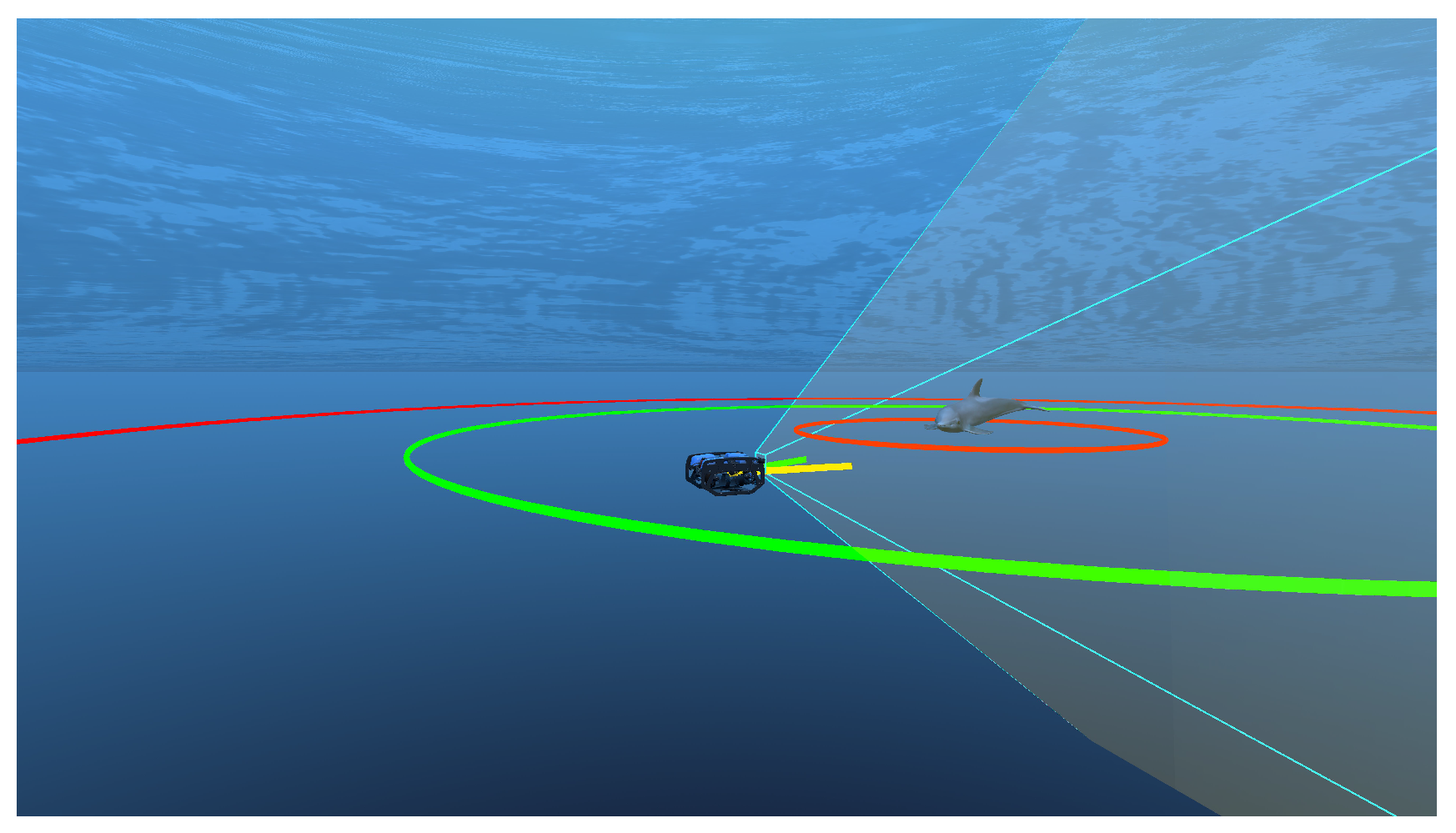
- Target Visibility. A stable and clear video feed is vital for providing meaningful feedback to marine conservation experts. Therefore, the target object should deviate little from the camera’s central field of view.
- Target Distance. Many marine populations are sensitive to disturbances caused by robotic monitoring. BLUEROV’s restricted target distance helps to avoid potential stress of discomfort that may be caused by a AUV with a stricter range threshold. In addition, we advocate that freedom of movement is encouraged, capturing more of the environment and providing a greater environmental context.
- Collision Avoidance. The rover should avoid collisions with the target, preventing stress or panic in the animal and avoiding damage to the ROV, resulting in challenging autonomous control recovery.
- Smooth Control. DRL algorithms applied in real-time environments are particularly susceptible to jitter, as the target policy fails to infer velocity and aims only to achieve the current optimum.
- Pipeline Requirements. Sim-to-real transfer should minimise training time and reduce the costs and danger associated with real-world training. Our training pipeline should (1) minimise training time, (2) minimise hardware demand, and (3) exploit modern state-of-the-art solutions.
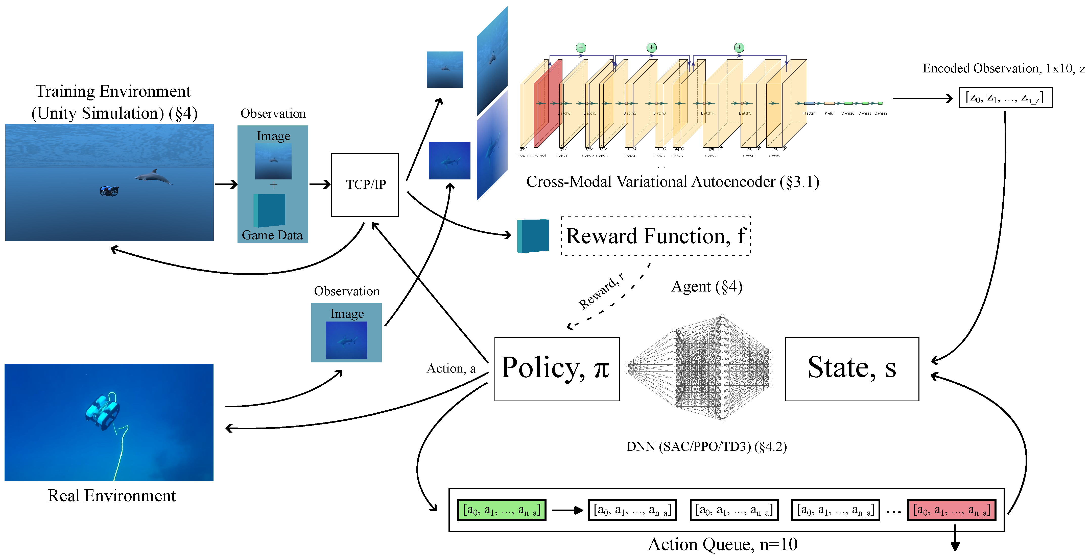
1.3. Methodology and Pipeline (Figure 1)
1.4. Improvements from SWiMM1.0
1.4.1. Target Visibility
1.4.2. Target Distance
1.4.3. Smooth Control
1.4.4. System Compatibility and Enhancements
1.4.5. Training Time
1.4.6. Benchmarking Correctness
2. Related Work
2.1. Unity
- Position. A translation matrix moves p to by v:
- Rotation. A rotation matrix rotates p to : , where depend on the rotated dimension.
- Forward. The forward vector, defines the z-facing direction vector (derivable from rotation).
2.2. Data
2.3. ML
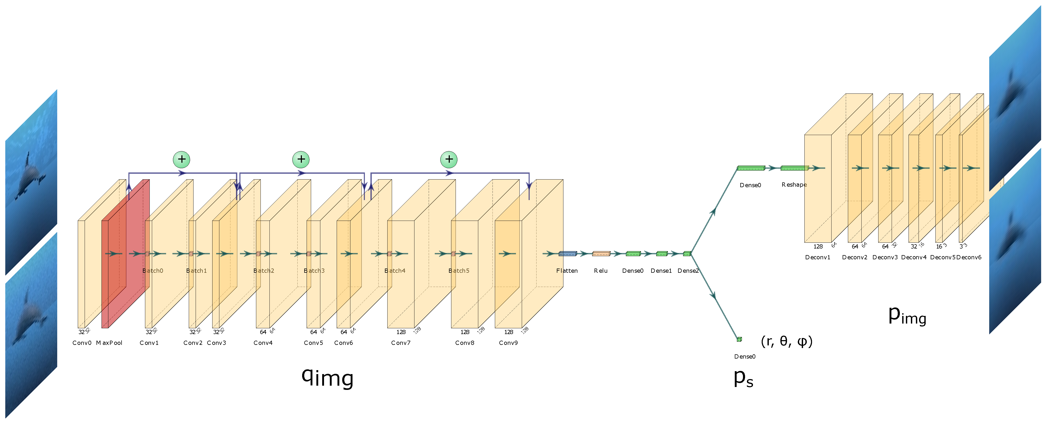
2.3.1. Feature Embedding
- Decoder, . reconstructs an image from z, consisting of six transposed convolutional layers, exploiting the ReLU activation function and batch normalisation before each convolution, providing the image reconstruction loss against the original image.
- State Decoder, . A set of auxiliary networks [31] (one per feature: d; and ) performs pose regression—predicting d, and . Each network consists of 2 dense layers. During training, each relevant feature from z is passed through , and losses between the ground truth and predicted feature values influence the gradient updates of , disentangling the learnt feature space and ensuring the first three features are task-relevant.
2.3.2. Three-Dimensional Object Tracking
2.3.3. RL
- Behaviour Policy: enforces the agent’s action for the current state in the current timestep .
- Target Policy: is updated based on the rewards from the current action. It is used to ‘learn’ the best action based on future rewards. These policies are often greedy.
- On-policy. the behaviour policy is the same as the target policy, . Therefore, the action proposed by the target policy (often a greedy policy estimating future rewards) is chosen.
- Off-policy. the behaviour policy can be different to the target policy, . For example, our behaviour policy may be random, while the target policy may follow a -greedy approach.
- SAC (off-policy) [37]: This is an actor-critic approach optimizing both policy and value network—a model estimating the expected return of a given state or state-action pair. It maximises a trade-off between expected cumulative reward and entropy (a measure of policy stochasticity), encouraging exploration by penalizing overly deterministic policies while maximizing expected rewards.
- PPO (on-policy) [17]: This provides a policy gradient solution improving training stability and efficiency by using a clipped objective function to limit the extent of policy updates.
- TD3 (off-policy) [18]: This combines aspects from Q-learning and policy gradients and has been exploited in advancing RL applications in continuous control tasks, such as robotic manipulation and autonomous driving.
3. Materials and Methods
3.1. Methodology
3.1.1. Deep Reinforcement Learning Pipeline
Observation Space
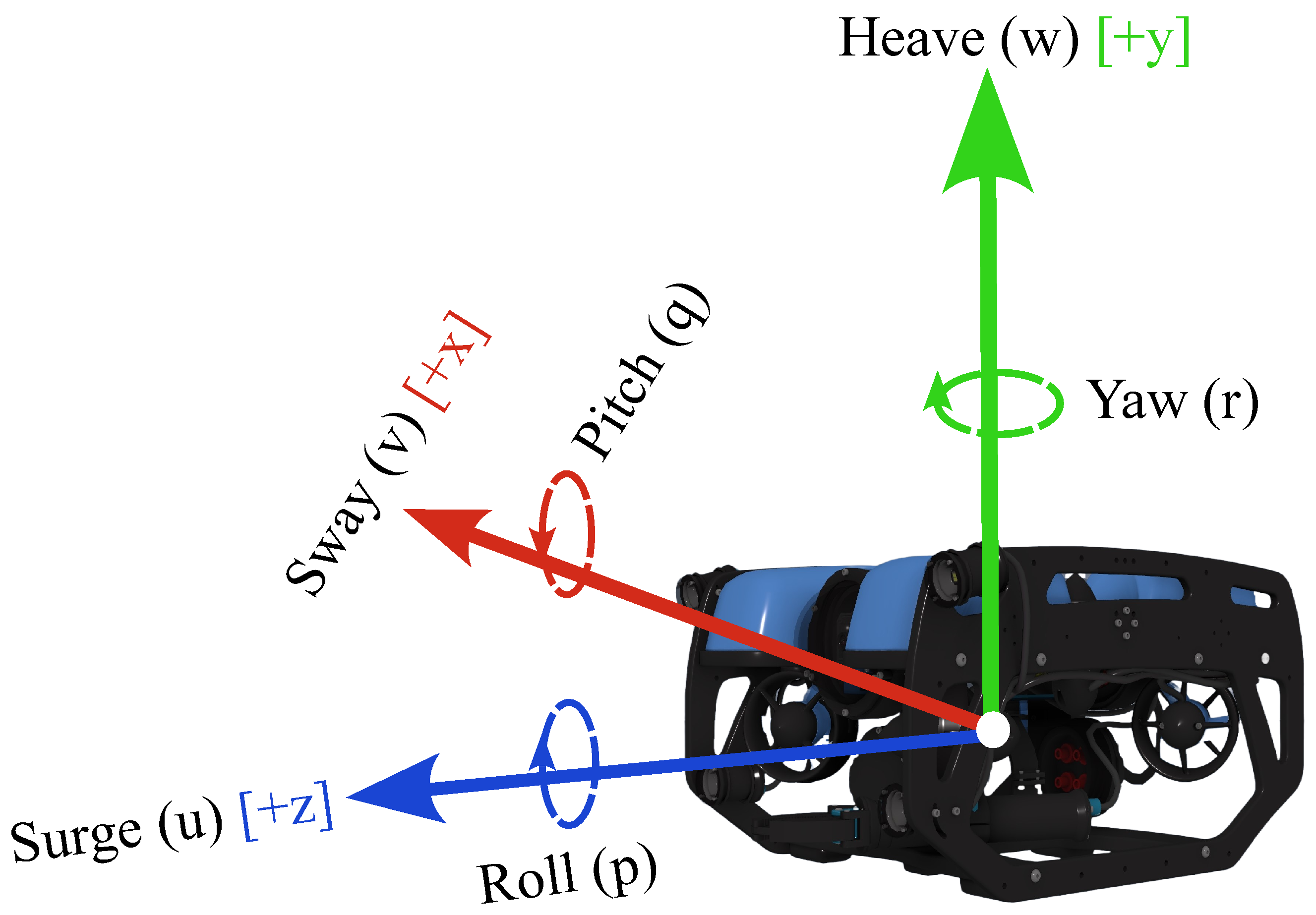
Action Space
- : No feedback stabilisation, heading holding or depth holding.
- : Roll is stabilised and yaw when not commanded to turn.
- : As but also will maintain heave unless commanded otherwise.
Reward Function,
- Distance Strictness, . In SWiMM1.0, was too great (scaling penalty quadratically), over-biasing the agent to achieve optimum distance while also causing greater changes to azimuth, thus leading to poor responsiveness. Instead, we should allow greater freedom of movement from opt_d as the video feedback (and, therefore, the penalty for azimuth increases) is affected more by the ROV’s heading than the raw distance. This also has the added benefit of minimising azimuth fluctuations. We replace the quadratic penalty with an exponential one; a more lenient behaviour.
- Poor Responsiveness, . To enforce a stricter heading penalty, we provide a logarithmic increase, rather than a linear one as in SWiMM1.0. For the latter, subsequent experiments reveal unresponsiveness to significant azimuth changes concerning the original maximum possible azimuth of 180°, which were not considering the camera’s horizontal field-of-view :where stands for camera sensor’s width. This new penalty encourages a much more responsive agent.
- Smooth Control. An agent penalised heavily for small changes from the optimum will jitter, whereby the action will continuously flip between negative and positive values. The challenge, then, is discovering an agent that can maintain optimum heading and distance while eliminating jitter caused by overshooting at the optimums. Preliminary investigations applying a smoothness penalty resulted in an agent being overly conscientious of maintaining smooth control. While the resulting policy almost eliminated jitter, sharp control changes were lacking, and the target was not tracked effectively. We opted for a different mechanism by extending the observation space to include the previous n actions (action stacking, distinct from frame stacking, Section ‘Observation Space’), which successfully eliminated jitter/overshooting. This is detailed in the following section, ‘Smoothness Error Implementation’.
Smoothness Error Implementation
Episode Termination
3.2. Simulation Engine
3.2.1. Environment Wrappers
- Episodes lasting longer than the threshold length indicate that the target policy has already been optimised for the current sequence of states. It is better to reset the environment to a set of new (potentially unobserved) states than to continue the current episode, continually receiving states already in the replay/rollout buffer.
- Resetting the environment results in state configurations that are unlikely to be observed once an episode has begun. This includes the starting and early states, where the ROV/target may have greatly varying velocities than those exhibited mid-episode.
3.2.2. Callbacks
- Rollout-Based Evaluation. Regarding agent performance, we advocate evaluation only after model optimisation. Evaluation on an episode threshold means several evaluations can be made for identical networks, which is not optimal.
- Step and Episode Threshold. Granted that continuous learning tasks are more concerned with step reward against the conditions at the end of an episode, we also allow step-based evaluation frequencies to support continuous learning tasks.
- Minimum Steps for Evaluation. DRL networks, and therefore the target policy, are more susceptible to large changes in behaviour during the early stages of training (particularly with dynamic learning rates that anneal with time). Given that this (inexperienced) behaviour has been trained only on a limited number of samples, we provide a new criterion, a minimum training step threshold, that must be reached before evaluation can begin.
3.2.3. Physics
Buoyancy
3.2.4. Reproducibility
Freeze Pipeline
- First. Native Unity physics is disabled.
- Second. We perform a physics update for the rover/target. For the former, actions from the DRL network provide the emulated joystick controls, while the latter integrates the forces as determined by its state machine.
- Third. We await the end of the current rendering step. At this point, physics and graphics are synchronised and the resulting image accurately represents the physical characteristics.
- Fourth. Game data are retrieved, including the positions and rotations of the rover/target. Both the game data and image render are encoded into an observation, which is then sent back across the TCP/IP socket.
- Fifth. Repeat 2–4 until commanded by the network otherwise.
| Algorithm 1: Freeze Pipeline Implementation |
 |
Network
BLUEROV Modelling
Mesh
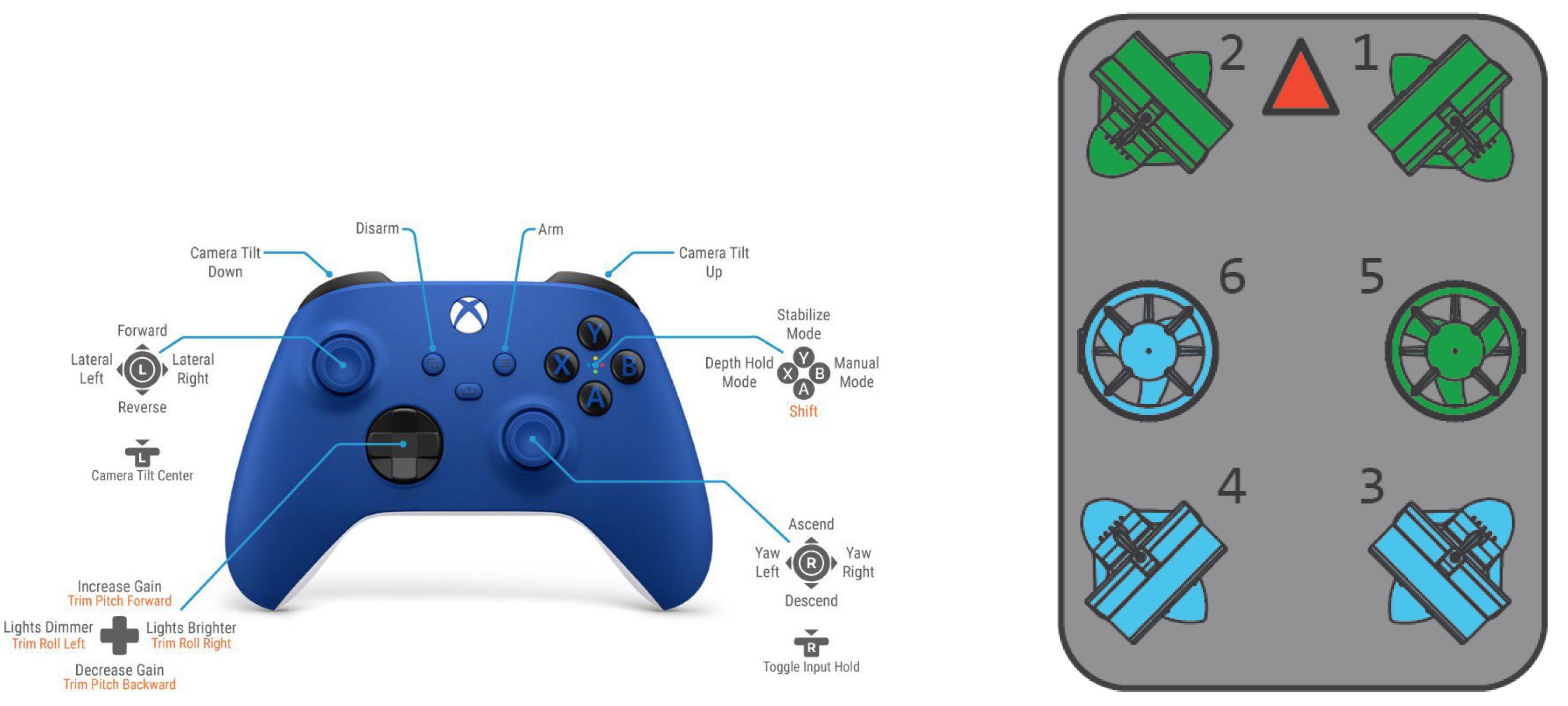
Controls
Action Inference
- Δ
- maintain. Every action is applied for all simulation ticks in between actions.
- Δ
- onReceive. Each action is enforced for one simulation tick only. The observer then waits for the next command.
- ★
- freeze. Each action is enforced for one simulation tick only. Native physics behaviour is disabled. Upon receiving an action, our custom physics step is exploited, guaranteeing simulation consistency. Detailed implementation is described in Section 3.2.4.
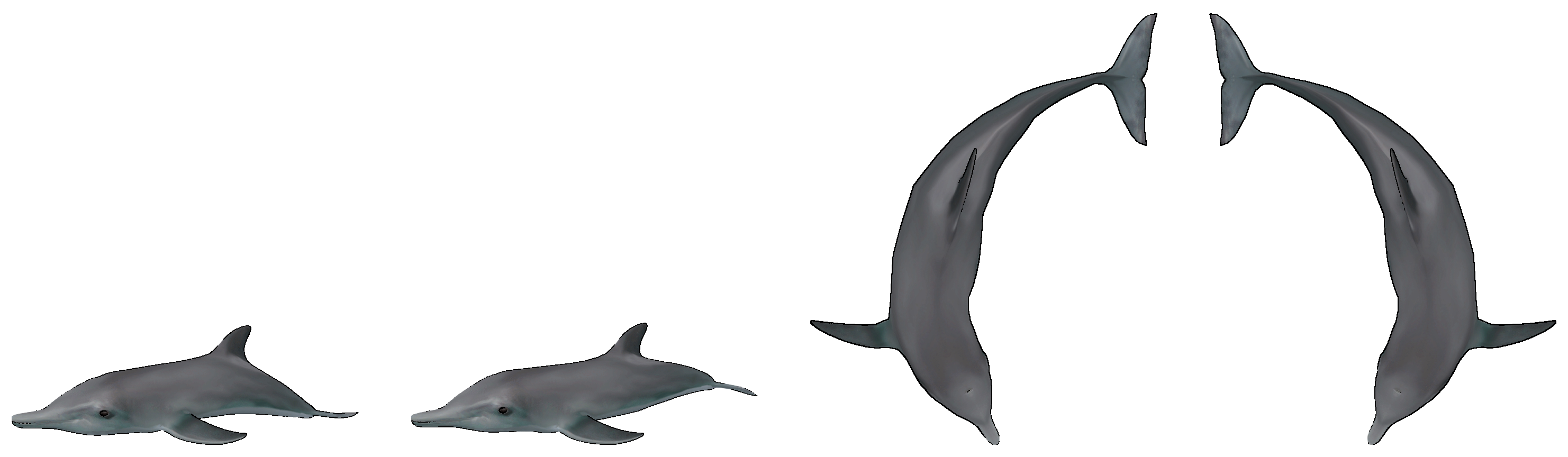
3.2.5. Target Modelling
- Undulatory Locomotion. Sinusoidal movement along the bodies and tails provides forward movement.
- Rolling. Enables more efficient water navigation.
- Yawing. Bending and flexing of bodies changes direction.
4. Results
- DRL network weight initialisation. Network weight initialisation is well known to impact a network’s optimisation, evidenced by our DRL experiments.
- CMVAE sampling strategy. Values sampled by our decoder are obtained from normal random distributions.
- DRL action determinism. A multilayer perceptron policy for each SAC/PPO/TD3 represent non-deterministic policies.
- Simulation Randomisation. Unity exploits random number generators, determining the environment’s initial and reset state (positions, orientations, etc.).
4.1. Data Generation Setup
4.2. Image Similarity
- Texture Rendering. The cost of rendering high-resolution images is high, from both a memory and time perspective, in particular for sample-hungry DRL algorithms.
- Message Latency. Latency defines the ratio between message size and throughput of our TCP connection. High-resolution image vectors necessitate large buffer size requirements, introducing a significant delay between observation and control commands.
- Can we exploit image scaling techniques in Unity to reduce network traffic latency?
- If above, can we render our input resolution directly, reducing rendering load?
4.3. CMVAE Training
- Early Stopping. To prevent any unnecessary training providing no benefit to models having already found a maximum optimum [42], we monitor validation losses concerning a window size . Where no monitoring exists, we denote this as , otherwise, an integer n indicates the patience value.
4.3.1. Training
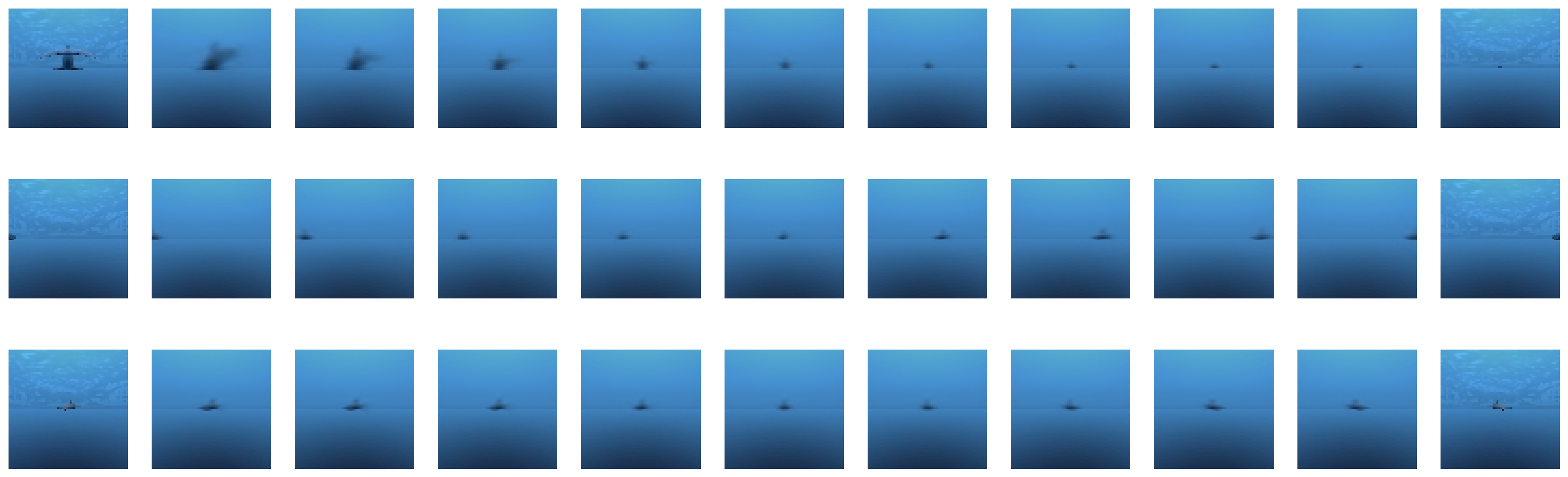
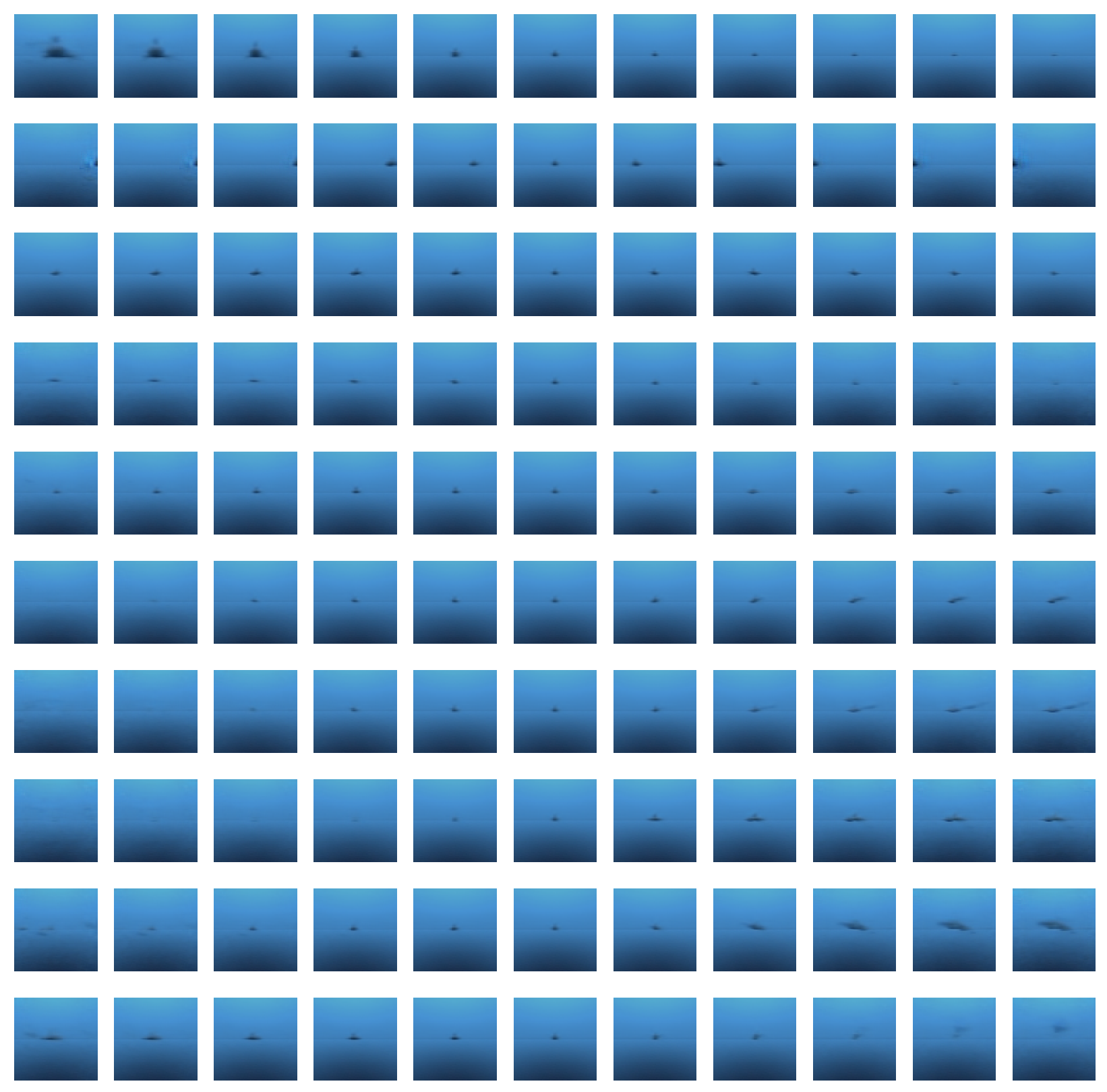
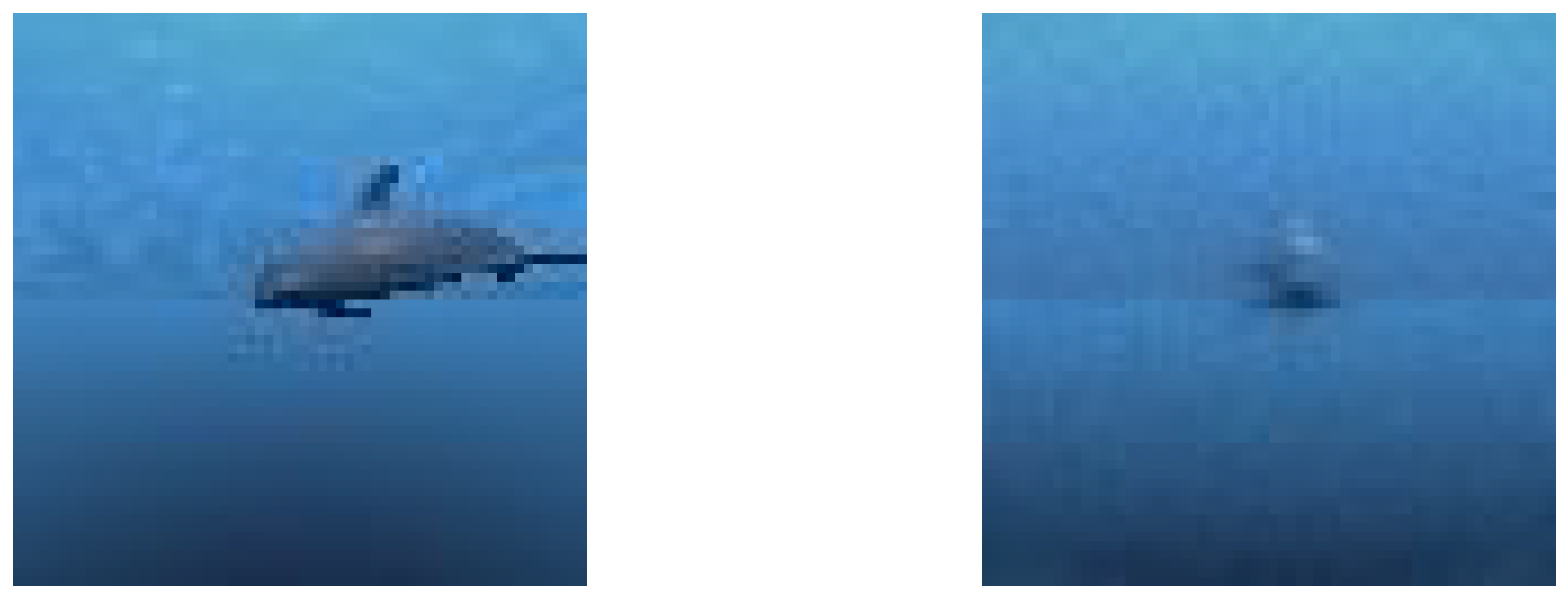
4.3.2. Inference
4.4. Reinforcement Learning
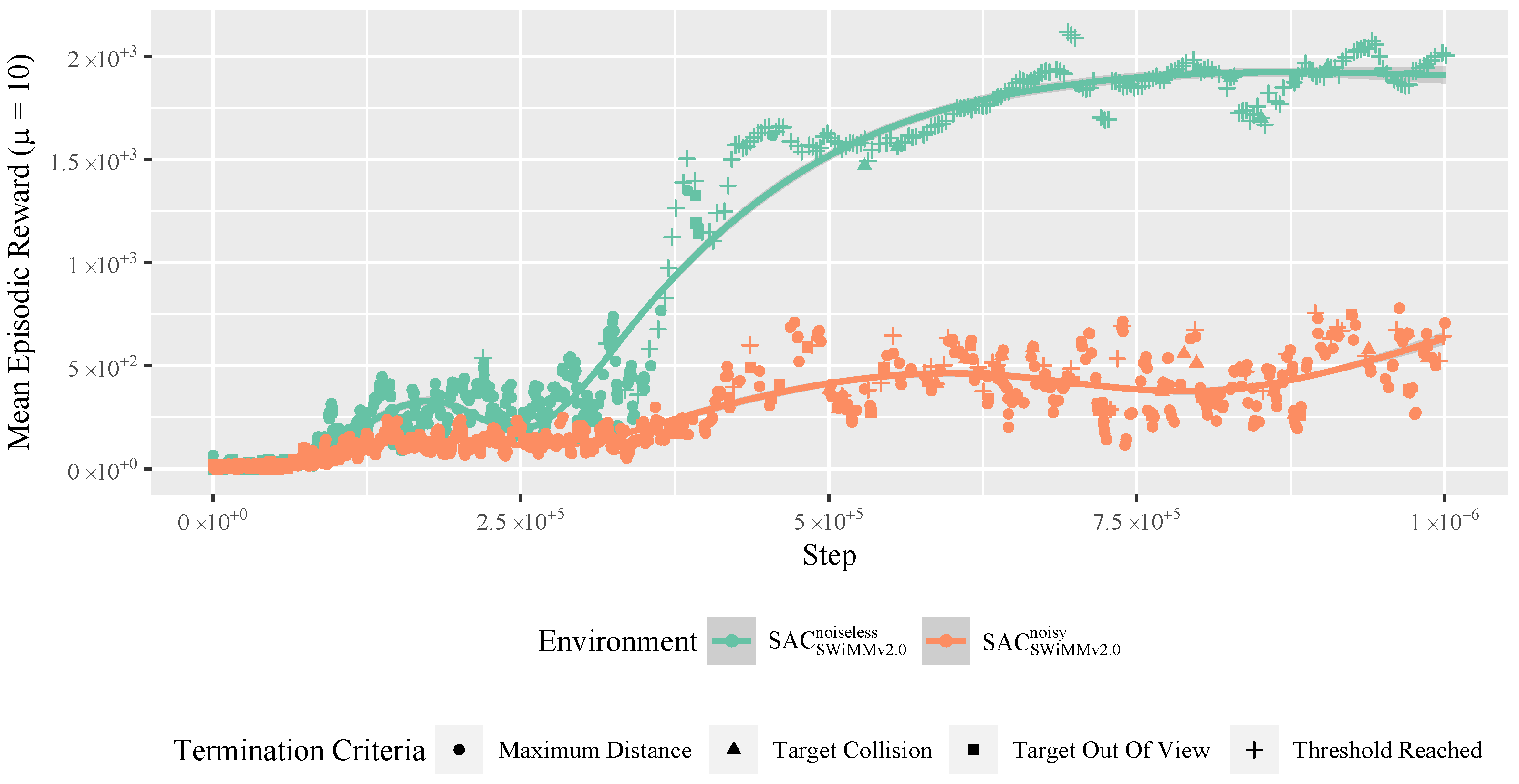
4.4.1. Training
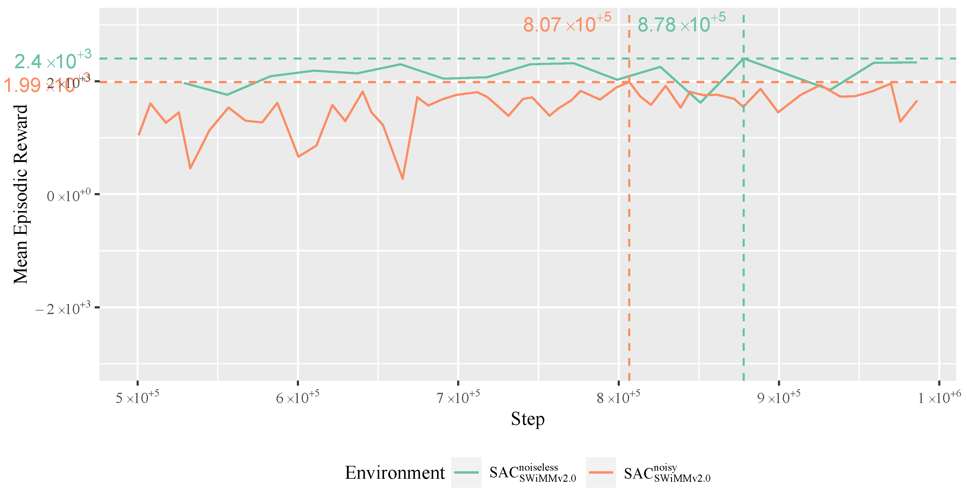
4.4.2. Evaluation
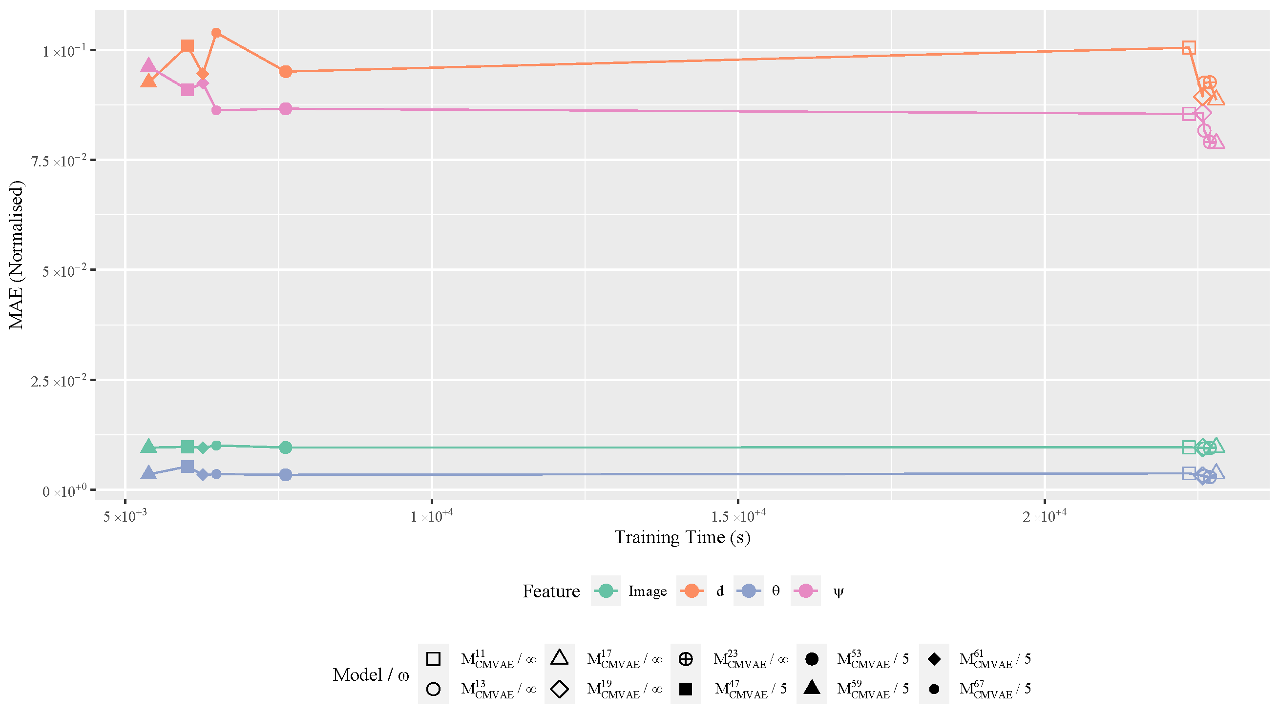
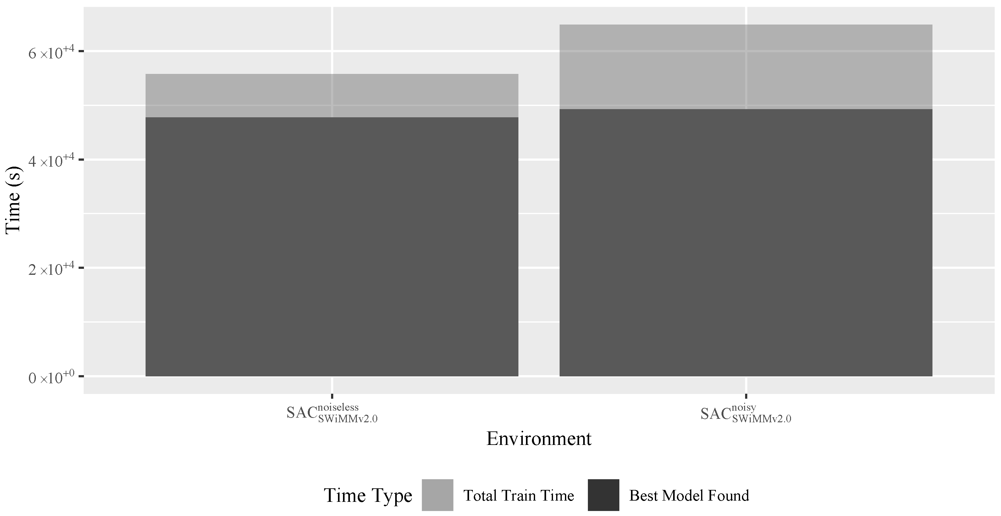
4.4.3. Training Times
Training Time Influencing Factors
- Model Performance. Well-behaving models regularly achieve the maximum episode length, while a poorly behaving one activates some of our episode termination criteria (Table 4). The latter, activating early episode termination, results in lower FPS, due to the high resource demand of environment reset.
- Network Optimisation Frequency. While SAC performs network updates per episode, PPO/TD3 perform theirs every 512 step. Therefore, the latter exhibits an (almost) constant number of updates per run, while the former performs an indeterminable number of updates. Well-performing models will suffer from the latter due to the more regular (and unnecessary) updating of network weights.
- Network Architecture. SAC/PPO/TD3 exploit different network architectures (Section 4.4.1), in both the number of hidden layers and neurons per layer. More complex networks have a higher resource demand.
- Algorithmic Implementation. TD3 exploits twinned critics while SAC and PPO exploit only one, doubling the demand on critic network optimisation.
Training Time Benchmarks
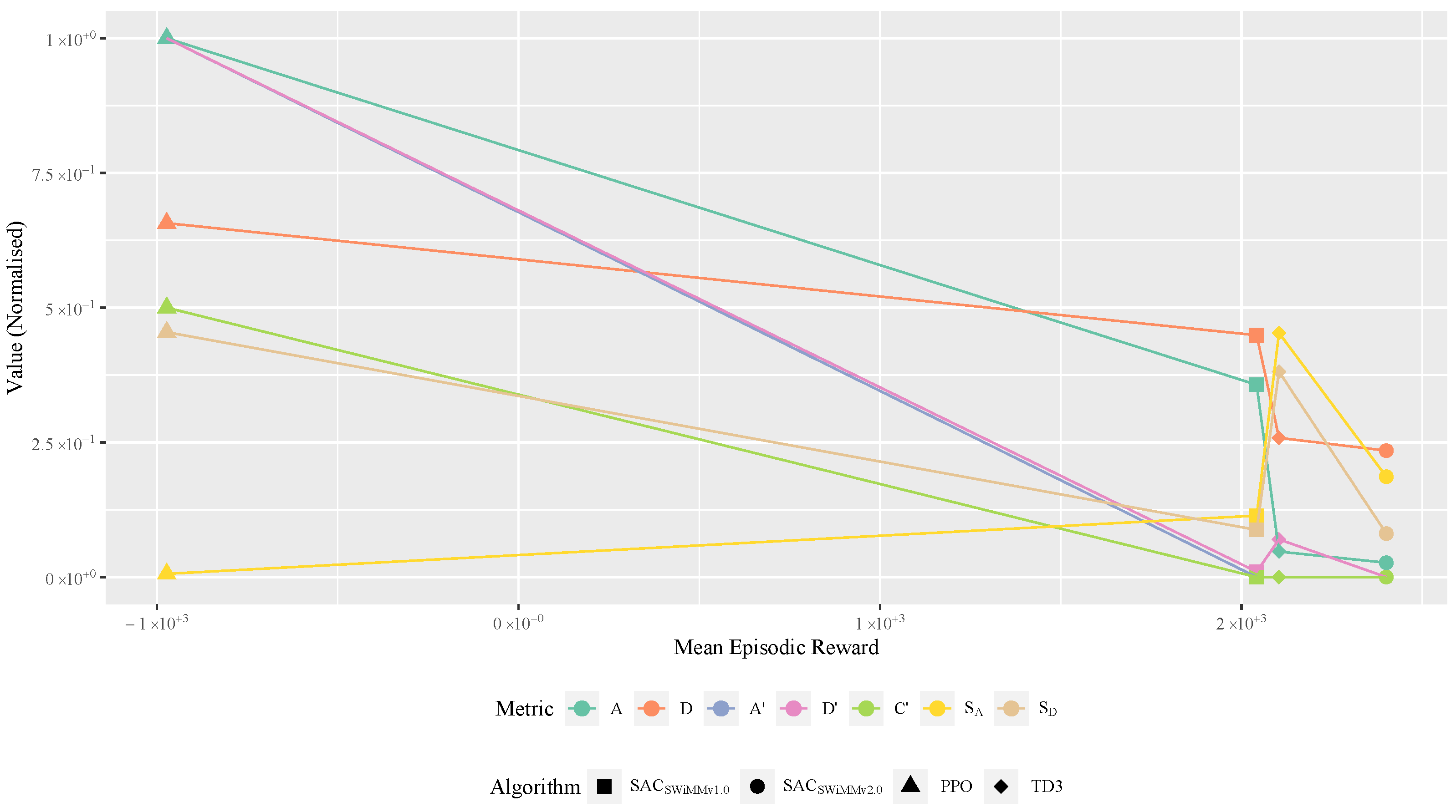
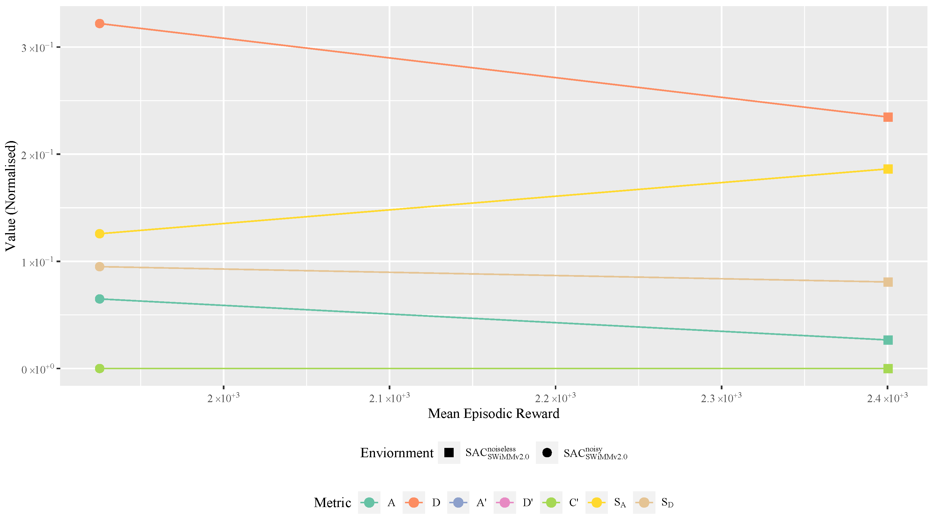
4.4.4. Model Behaviour Metrics
4.4.5. Inference
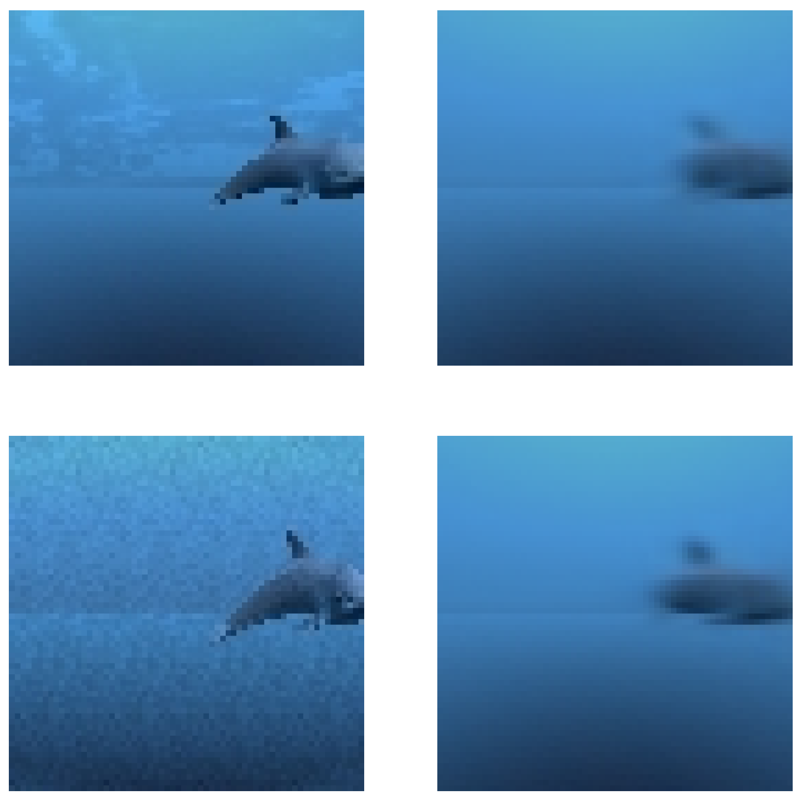
4.4.6. Model Robusteness to Noise
- Enhanced Fog: Unity fog overlays colour onto pixels concerning their distance from the camera. Our enhanced fog exploits the squared exponential distance. This enables a much greater emphasis on a murky underwater effect in contrast with SWiMM1.0, which used exponential with lesser weight only.
- Grain: Grain exploits a gradient coherent-noise function to simulate irregularities in film tape. In our simulation, we exploit grain to emulate stochastic underwater particles particularly those causing reflection.
- Depth of Field: This simulates the focusing properties of a camera lens, enabling physically accurate Bokeh depth of field effects.
- Lens Distortion: Warps pixel data to make objects bend inward (pincushion distortion) or outward (barrel distortion). We provide barrel distortion to emulate underwater fisheye lens.
- Motion Blur: When objects move faster than a camera’s exposure time, they are blurred. We provide a camera-based motion blur.
5. Discussion
5.1. CMVAE/DRL Training Decoupling
5.2. Headless Mode Optimisations
5.3. Seeding and Reproducibility
5.4. Limitations
5.4.1. DRL Robustness
5.4.2. Noise Type Volatility
5.5. Additional Sensors
6. Conclusions and Future Work
Supplementary Materials
Author Contributions
Funding
Institutional Review Board Statement
Informed Consent Statement
Data Availability Statement
Acknowledgments
Conflicts of Interest
Abbreviations
| AUV | autonomous underwater vehicle |
| BLUEROV | BlueROV2 |
| CMVAE | cross-modal variational autoencoder |
| CNN | convolutional neural network |
| DNN | deep neural network |
| DRL | deep reinforcement learning |
| FPS | frames per second |
| L2D | learning to drive |
| MAE | mean absolute error |
| ME | max error |
| ML | machine learning |
| PPO | proximal policy optimisation |
| RL | reinforcement learning |
| ROV | remote-operated vehicle |
| RTF | real-time factor |
| SAC | soft actor critic |
| SE | standard error |
| SWIM | SWiMM DEEPeR |
| TD3 | twin delayed deep deterministic policy gradients |
| UUV | unmanned underwater vehicle |
| UVMS | underwater vehicle manipulator system |
| VAE | variational autoencoder |
| VARG | video action recongition networks |
Nomenclature
| Notation | Description | Unit |
|---|---|---|
| SWiMM2.0 | SWiM v2.0 | |
| SWiMM1.0 | SWiM v1.0 | |
| z | latent space vector | → |
| s | state | |
| r | reward | |
| reward function | ||
| target policy | ||
| d | distance | |
| transform | ||
| image encoder | ||
| image decoder | ||
| state decoder | ||
| azimuth | ||
| target rotation | ||
| o | observation | → |
| a | action | → |
| behaviour policy | ||
| exploration probability | ||
| ActPrev | list of the previous 10 actions | |
| W | image width | |
| H | image height | |
| dimension of z | ||
| BLUEROV dive mode | ||
| opt_d | optimum distance | |
| max_d | maximum distance | |
| distance penalty | ||
| azimuth penalty | ||
| camera horizontal field-of-view | ||
| camera sensor width | ||
| f | focal length | |
| half the camera horizontal field-of-view | ||
| Δ | Unity-based physics | |
| ★ | custom physics | |
| a model saved with a seed, , saved at a timestamp | ||
| cmvae training set | ||
| cmvae test set | ||
| image interpolation set | ||
| image validation set | ||
| C | number of colour channels | |
| pixel at a width w and height h | ||
| retain the previous episodes for early stopping | ||
| best trained CMVAE | ||
| SACSWiMMv1.0 | previous best SAC model | |
| SACSWiMMv2.0 | current best SAC model | |
| stats_window_size | retain the previous stats_window_size episodes for monitoring | |
| network architecture | ||
| mean distance error | ||
| mean azimuth error | ||
| target collision count | ||
| distance threshold exceeded count | ||
| target visibility count | ||
| surge smoothness error | ||
| yaw smoothness error | ||
| SACSWiMMv2.0 model trained on a noisy environment | ||
| SACSWiMMv2.0 model trained on a noisy environment |
References
- Wells, R.; Early, G.; Gannon, J.; Lingenfelser, R.; Sweeney, P. Tagging and Tracking of Rough-Toothed Dolphins (Steno bredanensis) from the March 2005 Mass Stranding in the Florida Keys; NOAA Technical Memorandum; National Oceanic and Atmospheric Administration (NOAA): Washington, DC, USA, 2008. Available online: https://repository.library.noaa.gov/view/noaa/8656 (accessed on 21 March 2025).
- Sequeira, A.M.M.; Heupel, M.R.; Lea, M.A.; Eguíluz, V.M.; Duarte, C.M.; Meekan, M.G.; Thums, M.; Calich, H.J.; Carmichael, R.H.; Costa, D.P.; et al. The importance of sample size in marine megafauna tagging studies. Ecol. Appl. 2019, 29, e01947. [Google Scholar] [CrossRef]
- Inzartsev, A.V. Underwater Vehicles; IntechOpen: Rijeka, Croatia, 2009. [Google Scholar]
- Wynn, R.B.; Huvenne, V.A.; Le Bas, T.P.; Murton, B.J.; Connelly, D.P.; Bett, B.J.; Ruhl, H.A.; Morris, K.J.; Peakall, J.; Parsons, D.R.; et al. Autonomous Underwater Vehicles (AUVs): Their past, present and future contributions to the advancement of marine geoscience. Mar. Geol. 2014, 352, 451–468. [Google Scholar]
- Liu, Y.; Anderlini, E.; Wang, S.; Ma, S.; Ding, Z. Ocean Explorations Using Autonomy: Technologies, Strategies and Applications. In Offshore Robotics; Springer: Singapore, 2022; pp. 35–58. [Google Scholar]
- von Benzon, M.; Sørensen, F.F.; Uth, E.; Jouffroy, J.; Liniger, J.; Pedersen, S. An Open-Source Benchmark Simulator: Control of a BlueROV2 Underwater Robot. J. Mar. Sci. Eng. 2022, 10, 1898. [Google Scholar] [CrossRef]
- Yang, X.; Xing, Y. Tuning for robust and optimal dynamic positioning control in BlueROV2. IOP Conf. Ser. Mater. Sci. Eng. 2021, 1201, 012015. [Google Scholar] [CrossRef]
- Walker, K.; Gabl, R.; Aracri, S.; Cao, Y.; Stokes, A.; Kiprakis, A.; Giorgio Serchi, F. Experimental Validation of Wave Induced Disturbances for Predictive Station Keeping of a Remotely Operated Vehicle. IEEE Robot. Autom. Lett. 2021, 6, 5421–5428. [Google Scholar] [CrossRef]
- Skaldebø, M.; Schjølberg, I.; Haugaløkken, B.O. Underwater Vehicle Manipulator System (UVMS) with BlueROV2 and SeaArm-2 Manipulator. In International Conference on Offshore Mechanics and Arctic Engineering; American Society of Mechanical Engineers: New York, NY, USA, 2022; Volume 85901, p. V05BT06A022. [Google Scholar] [CrossRef]
- Katara, P.; Khanna, M.; Nagar, H.; Panaiyappan, A. Open Source Simulator for Unmanned Underwater Vehicles using ROS and Unity3D. In Proceedings of the 2019 IEEE Underwater Technology, Kaohsiung, Taiwan, 16–19 April 2019. [Google Scholar]
- Viitala, A.; Boney, R.; Zhao, Y.; Ilin, A.; Kannala, J. Learning to Drive (L2D) as a Low-Cost Benchmark for Real-World Reinforcement Learning. In Proceedings of the 2021 20th International Conference on Advanced Robotics (ICAR), Ljubljana, Slovenia, 6–10 December 2021; pp. 275–281. [Google Scholar] [CrossRef]
- Huang, Z.; Buchholz, M.; Grimaldi, M.; Yu, H.; Carlucho, I.; Petillot, Y.R. URoBench: Comparative Analyses of Underwater Robotics Simulators from Reinforcement Learning Perspective. In Proceedings of the OCEANS 2024-Singapore, Singapore, 15–18 April 2024; pp. 1–8. [Google Scholar] [CrossRef]
- Potokar, E.; Ashford, S.; Kaess, M.; Mangelson, J. HoloOcean: An Underwater Robotics Simulator. In Proceedings of the 2022 International Conference on Robotics and Automation (ICRA), Philadelphia, PA, USA, 23–27 May 2022. [Google Scholar]
- Zhang, M.; Choi, W.S.; Herman, J.; Davis, D.; Vogt, C.; Mccarrin, M.; Vijay, Y.; Dutia, D.; Lew, W.; Peters, S.; et al. DAVE Aquatic Virtual Environment: Toward a General Underwater Robotics Simulator. In Proceedings of the 2022 IEEE/OES Autonomous Underwater Vehicles Symposium (AUV), Singapore, 19–21 September 2022; pp. 1–8. [Google Scholar] [CrossRef]
- Cieślak, P. Stonefish: An Advanced Open-Source Simulation Tool Designed for Marine Robotics, With a ROS Interface. In Proceedings of the OCEANS 2019-Marseille, Marseille, France, 17–20 June 2019; pp. 1–6. [Google Scholar] [CrossRef]
- Appleby, S.; Crane, K.; Bergami, G.; McGough, A.S. SWiMM DEEPeR: A Simulated Underwater Environment for Tracking Marine Mammals Using Deep Reinforcement Learning and BlueROV2. In Proceedings of the 2023 IEEE Conference on Games (CoG), Boston, MA, USA, 21–24 August 2023; pp. 1–8. [Google Scholar] [CrossRef]
- Schulman, J.; Wolski, F.; Dhariwal, P.; Radford, A.; Klimov, O. Proximal Policy Optimization Algorithms. arXiv 2017, arXiv:1707.06347. [Google Scholar]
- Fujimoto, S.; van Hoof, H.; Meger, D. Addressing Function Approximation Error in Actor-Critic Methods. In Proceedings of the International Conference on Machine Learning, Macau, China, 26–28 February 2018. [Google Scholar]
- Kaufmann, E.; Bauersfeld, L.; Loquercio, A.; Müller, M.; Koltun, V.; Scaramuzza, D. Champion-level drone racing using deep reinforcement learning. Nature 2023, 620, 982–987. [Google Scholar] [CrossRef]
- Rolland, R.M.; Parks, S.E.; Hunt, K.E.; Castellote, M.; Corkeron, P.J.; Nowacek, D.P.; Wasser, S.K.; Kraus, S.D. Evidence that ship noise increases stress in right whales. Proc. R. Soc. B Biol. Sci. 2012, 279, 2363–2368. [Google Scholar] [CrossRef]
- Gregory, J. Game Engine Architecture, 3rd ed.; A K Peters/CRC Press: Boca Raton, FL, USA, 2018. [Google Scholar]
- Juliani, A.; Berges, V.P.; Teng, E.; Cohen, A.; Harper, J.; Elion, C.; Goy, C.; Gao, Y.; Henry, H.; Mattar, M.; et al. Unity: A general platform for intelligent agents. arXiv 2020, arXiv:1809.02627. [Google Scholar]
- Zhao, W.; Queralta, J.P.; Westerlund, T. Sim-to-real transfer in deep reinforcement learning for robotics: A survey. In Proceedings of the 2020 IEEE symposium series on computational intelligence, Canberra, Australia, 1–4 December 2020; pp. 737–744. [Google Scholar]
- Maglietta, R.; Fanizza, C.; Cherubini, C.; Bellomo, S.; Carlucci, R.; Dimauro, G. Risso’s Dolphin Dataset. IEEE Dataport 2023. [Google Scholar] [CrossRef]
- Maglietta, R.; Bussola, A.; Carlucci, R.; Fanizza, C.; Dimauro, G. ARIANNA: A novel deep learning-based system for fin contours analysis in individual recognition of dolphins. Intell. Syst. Appl. 2023, 18, 200207. [Google Scholar] [CrossRef]
- Zhivomirov, H.; Nedelchev, I.; Dimitrov, G. Dolphins Underwater Sounds Database. TEM J. 2020, 9, 1426. [Google Scholar] [CrossRef]
- Frasier, K.E. A machine learning pipeline for classification of cetacean echolocation clicks in large underwater acoustic datasets. PLoS Comput. Biol. 2021, 17, e1009613. [Google Scholar] [CrossRef]
- Trotter, C.; Atkinson, G.; Sharpe, M.; Richardson, K.; McGough, A.S.; Wright, N.; Burville, B.; Berggren, P. NDD20: A large-scale few-shot dolphin dataset for coarse and fine-grained categorisation. arXiv 2020, arXiv:2005.13359. [Google Scholar]
- Kingma, D.P.; Welling, M. An introduction to variational autoencoders. arXiv 2019, arXiv:1906.02691. [Google Scholar]
- Spurr, A.; Song, J.; Park, S.; Hilliges, O. Cross-Modal Deep Variational Hand Pose Estimation. In Proceedings of the 2018 IEEE/CVF Conference on Computer Vision and Pattern Recognition (CVPR), Los Alamitos, CA, USA, 15–20 June 2018; pp. 89–98. [Google Scholar] [CrossRef]
- Bonatti, R.; Madaan, R.; Vineet, V.; Scherer, S.; Kapoor, A. Learning visuomotor policies for aerial navigation using cross-modal representations. In Proceedings of the 2020 IEEE/RSJ International Conference on Intelligent Robots and Systems (IROS), Las Vegas, NV, USA, 24 October 2020–24 January 2021; pp. 1637–1644. [Google Scholar]
- Loquercio, A.; Maqueda, A.I.; Del-Blanco, C.R.; Scaramuzza, D. Dronet: Learning to fly by driving. IEEE Robot. Autom. Lett. 2018, 3, 1088–1095. [Google Scholar]
- Li, J.; Wang, B.; Ma, H.; Gao, L.; Fu, H. Visual Feature Extraction and Tracking Method Based on Corner Flow Detection. IECE Trans. Intell. Syst. 2024, 1, 3–9. [Google Scholar] [CrossRef]
- Wang, F.; Yi, S. Spatio-temporal Feature Soft Correlation Concatenation Aggregation Structure for Video Action Recognition Networks. IECE Trans. Sens. Commun. Control 2024, 1, 60–71. [Google Scholar] [CrossRef]
- Sidorenko, G.; Thunberg, J.; Vinel, A. Cooperation for Ethical Autonomous Driving. In Proceedings of the 2024 20th International Conference on Wireless and Mobile Computing, Networking and Communications (WiMob), Paris, France, 21–23 October 2024; pp. 391–395. [Google Scholar] [CrossRef]
- Abro, G.E.M.; Ali, Z.A.; Rajput, S. Innovations in 3D Object Detection: A Comprehensive Review of Methods, Sensor Fusion, and Future Directions. IECE Trans. Sens. Commun. Control 2024, 1, 3–29. [Google Scholar] [CrossRef]
- Haarnoja, T.; Zhou, A.; Abbeel, P.; Levine, S. Soft Actor-Critic: Off-Policy Maximum Entropy Deep Reinforcement Learning with a Stochastic Actor. arXiv 2018, arXiv:1801.01290. [Google Scholar]
- Mnih, V.; Kavukcuoglu, K.; Silver, D.; Rusu, A.A.; Veness, J.; Bellemare, M.G.; Graves, A.; Riedmiller, M.; Fidjeland, A.K.; Ostrovski, G.; et al. Human-level control through deep reinforcement learning. Nature 2015, 518, 529–533. [Google Scholar]
- Anzalone, L.; Barra, P.; Barra, S.; Castiglione, A.; Nappi, M. An End-to-End Curriculum Learning Approach for Autonomous Driving Scenarios. IEEE Trans. Intell. Transp. Syst. 2022, 23, 19817–19826. [Google Scholar] [CrossRef]
- Lapan, M. Deep Reinforcement Learning Hands-On: Apply Modern RL Methods to Practical Problems of Chatbots, Robotics, Discrete Optimization, Web Automation, and More; Packt Publishing: Birmingham, UK, 2020. [Google Scholar]
- Hays, G.C.; Ferreira, L.C.; Sequeira, A.M.; Meekan, M.G.; Duarte, C.M.; Bailey, H.; Bailleul, F.; Bowen, W.D.; Caley, M.J.; Costa, D.P.; et al. Key Questions in Marine Megafauna Movement Ecology. Trends Ecol. Evol. 2016, 31, 463–475. [Google Scholar] [CrossRef]
- Yao, Y.; Rosasco, L.; Caponnetto, A. On Early Stopping in Gradient Descent Learning. Constr. Approx. 2007, 26, 289–315. [Google Scholar] [CrossRef]
- Yao, S.; Zhao, Y.; Shao, H.; Liu, S.; Liu, D.; Su, L.; Abdelzaher, T. FastDeepIoT: Towards Understanding and Optimizing Neural Network Execution Time on Mobile and Embedded Devices. In Proceedings of the 16th ACM Conference on Embedded Networked Sensor Systems, SenSys ’18, New York, NY, USA, 4–7 November 2018; pp. 278–291. [Google Scholar] [CrossRef]
- Mnih, V.; Kavukcuoglu, K.; Silver, D.; Graves, A.; Antonoglou, I.; Wierstra, D.; Riedmiller, M. Playing Atari with Deep Reinforcement Learning. arXiv 2013, arXiv:1312.5602. [Google Scholar]


| Benzon et al. [6] | Yang et al. [7] | Walker et al. [8] | Skaldebo et al. [9] | Viitala et al. [11] | SWiMM2.0 | |
|---|---|---|---|---|---|---|
| Engine | Matlab/Simulink | Matlab/Simulink | Matlab | Gazebo | Unity | Unity |
| Purpose | Physical modelling | Dynamic positioning control | Wave-induced disturbances | Underwater vehicle manipulator system | Image-based track following | Image-based marine megafauna monitoring |
| Robot | BLUEROV | BLUEROV | BLUEROV | BLUEROV | Donkey Car | BLUEROV |
| Sim-to-Real | ✓ | ✓ | ✓ | ✓ | ✓ | ✓ |
| Physical Camera Modelling | ✗ | ✗ | ✗ | ✓ | ✓ | ✓ |
| RL Support | ✗ | ✗ | ✗ | ✗ | ✓ | ✓ |
| Observation Type | Dimensionality | SWiMM1.0 | SWiMM2.0 |
|---|---|---|---|
| Ground Truth | 12 | rov/target | SWiMM1.0 + ActPrev |
| Raw Image | |||
| Encoded Image |
| Function | SWiMM1.0 | SWiMM2.0 |
|---|---|---|
| 1. | ||
| 2. | ||
| Parameter | Definition | Value | SWiMM1.0 | SWiMM2.0 |
|---|---|---|---|---|
| Distance Threshold | A distance from the optimum no greater than the threshold should occur. | 4 | ✓ | ✓ |
| Target Visibility | The target should always be within view of the camera. | N/A | ✗ | ✓ |
| Collision Avoidance | A collision with the target must be avoided. | N/A | ✓ | ✓ |
| Time Limit | Episodes, , can run for, at most, s steps, . | ✓ | ✓ |
| Set | n | Resolutions () | Seed |
|---|---|---|---|
| 2 | |||
| 3 | |||
| 5 | |||
| 6 | 7 |
| Range (Unity x/y/z) | |
|---|---|
| Rover | |
| Position | |
| Rotation | |
| Target | |
| Euclidean Distance | |
| Rotation | |
| Forward Animation Weight | |
| Turn Animation Weight | |
| Normalised Animation State | |
| Parameter | Definition | Value | |
|---|---|---|---|
| cmvae_training_config | |||
| train_dir | Training samples directory (see Table 5) | ||
| batch_size | Size of splices for training data | 32 | 32 |
| learning_rate | Gradient learning rate | ||
| load_during_training | Should all images undergo splicing on the fly | True | True |
| max_size | Limit on number of samples | NULL | NULL |
| epochs | Maximum number of epochs to run | 100 | 100 |
| window_size | Epochs to analyse for early stopping criteria | 5 | NULL |
| loss_threshold | Fractional gain to reach within window_size | ||
| cmvae_global_config | |||
| use_cpu_only | Prevent GPU acceleration | False | False |
| n_z | Latent space size | 10 | 10 |
| img_res | Expected Resolution of Input Data | ||
| latent_space_constraints | Disentangle latent space constraints [31] | True | True |
| deterministic | Tensorflow determinism | True | True |
| env_config | |||
| … | |||
| seed | Seed exploited for stochastic operations | ||
| … | |||
| Env | |||
|---|---|---|---|
| Airsim | SWiMM1.0 | SWiMM2.0 | |
| d | |||
| Parameter | Definition | Value | |
|---|---|---|---|
| cmvae_inference_config | |||
| test_dir | Testing samples directory (see Table 5) | ||
| weights_path | Model’s network weights path | ||
| cmvae_global_config, see Table 7 | |||
| env_config | |||
| … | |||
| seed | Seed exploited for stochastic operations | ||
| … | |||
| Parameter | Definition | Value |
|---|---|---|
| cmvae_inference_config | ||
| … | ||
| weights_path | Path to the ‘best’ model’s network weights | |
| … | ||
| cmvae_global_config, see Table 7 | ||
| env_config | ||
| obs | Observation type | ‘cmvae’ |
| n_envs | Number of environments to run in parallel | 1 |
| img_res | Resolution of incoming images | |
| debug_logs | Should network logs be generated | FALSE |
| seed | Seed exploited for stochastic operations | |
| algorithm | DRL algorithm to train with | |
| render | Mode of rendering the Unity environment | ‘human’ |
| pre_trained_model_path | Model to either: train on-top of or to use for inference | ~ |
| env_wrapper | ||
| stable_baselines3.common.monitor.Monitor | ||
| allow_early_resets | Are we allowing early episode termination | TRUE |
| gymnasium.wrappers.time_limit.TimeLimit | ||
| max_episode_steps | Allow at most max_episode_steps per training episode | |
| callbacks | ||
| gym_underwater.callbacks.SwimEvalCallback | ||
| eval_inference_freq | How many episodes/steps to run the evaluation for | |
| eval_freq | Training episodes required per evaluation sequence | 10 |
| min_train_steps | Minimum number of training steps required to begin evaluation | |
| deterministic | Should the actor use deterministic or stochastic actions | TRUE |
| verbose | Output information and metrics | 1 |
| gym_underwater.callbacks.SwimCallback | ||
| Seed | Timestamp | Value | |
|---|---|---|---|
| SAC | 97 | ||
| 101 | |||
| 103 | |||
| 107 | |||
| 109 | |||
| PPO | 97 | ||
| 101 | |||
| 103 | |||
| 107 | |||
| 109 | |||
| TD3 | 97 | ||
| 101 | |||
| 103 | |||
| 107 | |||
| 109 |
| Objective (Section 1.2) | Symbol | Safety Condition | Formula (Normalised) |
|---|---|---|---|
| Objective 2 | ✗ | Mean d error | |
| Objective 1 | ✗ | Mean error | |
| Objective 2 | ✓ | Distance threshold exceeded (max 1 per episode) | |
| Objective 1 | ✓ | Target visibility lost (max 1 per episode) | |
| Objective 3 | ✓ | Total number of collisions (max 1 per episode) | |
| Objective 4 | ✗ | Mean distance smoothness error | |
| Objective 4 | ✗ | Mean yaw smoothness error |
| Parameter | Definition | Value |
|---|---|---|
| cmvae_inference_config, see Table 10 | ||
| cmvae_global_config, see Table 7 | ||
| env_config | ||
| obs | Observation type | ‘cmvae’ |
| n_envs | Number of environments to run in parallel | 1 |
| img_res | Resolution of incoming images | |
| debug_logs | Should network logs be generated | FALSE |
| seed | Seed exploited for stochastic operations | |
| algorithm | DRL algorithm to train with | |
| render | Mode of rendering the Unity environment | ‘human’ |
| pre_trained_model_path | Model to either: train on-top of or to use for inference | |
| env_wrapper, see Table 10 | ||
| callbacks | ||
| gym_underwater.callbacks.SwimEvalCallback | ||
| eval_inference_freq | How many episodes/steps to run the evaluation for | |
| eval_freq | Training episodes required per evaluation sequence | 10 |
| min_train_steps | Minimum number of training steps required to begin evaluation | |
| deterministic | Should the actor use deterministic or stochastic actions | TRUE |
| verbose | Output information and metrics | 1 |
| gym_underwater.callbacks.SwimCallback | ||
| Feature | MAE | Standard Error | Max Error |
|---|---|---|---|
| Image | |||
| r | |||
| MAE | SE | ME | |
|---|---|---|---|
| 0 | |||
| 1 | |||
| 2 | |||
| 3 | |||
| 4 | |||
| 5 | |||
| 6 | |||
| 7 | |||
| 8 | |||
| 9 |
Disclaimer/Publisher’s Note: The statements, opinions and data contained in all publications are solely those of the individual author(s) and contributor(s) and not of MDPI and/or the editor(s). MDPI and/or the editor(s) disclaim responsibility for any injury to people or property resulting from any ideas, methods, instructions or products referred to in the content. |
© 2025 by the authors. Licensee MDPI, Basel, Switzerland. This article is an open access article distributed under the terms and conditions of the Creative Commons Attribution (CC BY) license (https://creativecommons.org/licenses/by/4.0/).
Share and Cite
Appleby, S.; Bergami, G.; Ushaw, G. From Camera Image to Active Target Tracking: Modelling, Encoding and Metrical Analysis for Unmanned Underwater Vehicles. AI 2025, 6, 71. https://doi.org/10.3390/ai6040071
Appleby S, Bergami G, Ushaw G. From Camera Image to Active Target Tracking: Modelling, Encoding and Metrical Analysis for Unmanned Underwater Vehicles. AI. 2025; 6(4):71. https://doi.org/10.3390/ai6040071
Chicago/Turabian StyleAppleby, Samuel, Giacomo Bergami, and Gary Ushaw. 2025. "From Camera Image to Active Target Tracking: Modelling, Encoding and Metrical Analysis for Unmanned Underwater Vehicles" AI 6, no. 4: 71. https://doi.org/10.3390/ai6040071
APA StyleAppleby, S., Bergami, G., & Ushaw, G. (2025). From Camera Image to Active Target Tracking: Modelling, Encoding and Metrical Analysis for Unmanned Underwater Vehicles. AI, 6(4), 71. https://doi.org/10.3390/ai6040071