One-Shot Autoregressive Generation of Combinatorial Optimization Solutions Based on the Large Language Model Architecture and Learning Algorithms

Abstract

Large Language Models (LLMs) have immensely advanced the field of Artificial Intelligence (AI), with recent models being able to perform chain-of-thought reasoning and solve complex mathematical problems, ranging from theorem proving to ones involving advanced calculus. The success of LLMs derives from a combination of the Transformer architecture with its attention mechanism, the autoregressive training methodology with masked attention, and the alignment fine-tuning via reinforcement learning algorithms. In this research, we attempt to explore a possible solution to the fundamental NP-hard problem of combinatorial optimization, in particular, the Traveling Salesman Problem (TSP), by following the LLM approach in terms of the architecture and training algorithms. Similar to the LLM design, which is trained in an autoregressive manner to predict the next token, our model is trained to predict the next node in a TSP graph. After the model is trained on random TSP graphs with known near-optimal solutions, we fine-tune the model using Direct Preference Optimization (DPO). The tour generation in a trained model is autoregressive one-step generation with no need for iterative refinement. Our results are very promising and indicate that, for TSP graphs up to 100 nodes, a relatively small amount of training data yield solutions within a few percent of the optimal. This optimization improves if more data are used to train the model.

1. Introduction

Large Language Models (LLMs) have demonstrated impressive knowledge comprehension skills with the introduction of ChatGPT, and the follow-up models of Gemini, Llama, Claude, and, recently, DeepSeek, among others. While most of these excel at Natural Language Processing (NLP) tasks such as question answering, text comprehension, and summarization, more recent models have focused on improving their reasoning and mathematical understanding capabilities such as DeepSeek-R1 [1]. It has been demonstrated via benchmarks that DeepSeek-R1 surpasses average humans in complex mathematical reasoning. Since LLMs are trained on enormous amounts of data, an important question is, are these becoming really intelligent, or simply memorizing all the facts that have been presented to them during training? Since the LLMs are able to draw conclusions about complex problems using chain-of-reasoning processes, we explore a much more difficult problem in the context of an LLM’s learning capability, i.e., can the LLM model learn to predict a one-step solution to the combinatorial optimization problem? We explore this answer with respect to the learning of the solution to the Traveling Salesman Problem (TSP) by the existing Transformer-based architecture of an LLM and its learning and alignment by the reinforcement learning (RL) algorithm.

The TSP optimization problem can be described as, given n nodes and their (x,y) coordinates, determine a Hamiltonian cycle such that the total distance covered in the cycle (or tour) is lowest possible. The Hamiltonian cycle is defined as starting from a node, visiting each other node exactly once, and returning to the starting node at the end of the tour. Since there are $(n-1)!/2$ possible tours, the solution space to find the optimum greatly increases due to the factorial with respect to n. Because of this, and for its practical applicability, TSP optimization is an important problem in both theoretical Computer Science and industry. It is carried out in route planning for package deliveries, job scheduling, circuit layouts, and the airline and freight industries, among others. The optimization of TSP has been extensively studied in the last several decades both from mathematical as well as algorithmic perspectives. Since it is a provably NP-hard problem [2], only approximate solutions exist via metaheuristic evolutionary approaches.

In a metaheuristic approach, a population of candidate problem solutions is created initially (which are often random solutions). These are then evolved by following processes similar to behavior in nature (e.g., evolution in a Genetic Algorithm or foraging behavior in Ant Colony Optimization). Some of the important metaheuristic approaches to solving the TSP optimization include Genetic Algorithms [3,4], Simulated Annealing [5,6], Tabu Search [7,8], Particle Swarm Optimization [9,10], Ant Colony Optimization [11,12] and Memetic Algorithms [13,14]. Some approaches have attempted to use a hybrid of metaheuristic algorithms, e.g., [15,16]. The work in [15] used Particle Swarm Optimization, Ant Colony Optimization, and Three-Opt Algorithms to effectively optimize the TSP, while [16] combined Simulated Annealing and Tabu Search for a specialized version of the TSP optimization.

While different metaheuristics are able to provide a near-optimal solution to TSP graphs with up to a few hundred nodes, there are still some disadvantages in their approach. First is the evolutionary nature of all metaheuristic algorithms, which requires numerous iterations to refine the solution. For larger problems, the execution time increases greatly to arrive at a better solution. Because of the inherent iterative nature of the approach, the implementation of a metaheuristic algorithm can only be partially parallelized. Even though significant research has been carried out in parallelizing different metaheuristics, e.g., [12,17,18], the execution times for larger TSP instances can take many hours or even days of execution times. Additionally, in a metaheuristic algorithm, we need to balance the exploration of solutions in the search space with the exploitation (finding a better solution). Emphasizing the exploitation can lead to becoming stuck in local optima, while promoting more exploration can lead to oscillatory behavior, where solutions can become better and then worse fairly quickly.

The advancements in Artificial Intelligence via the use of Deep Learning algorithms and architectures offers a promising avenue for solving the TSP optimization in a more effective manner. We review some important works in this respect in the next section.

2. Related Work

One of the first important works with respect to combinatorial optimization by the use of Deep Learning was presented in [19], termed as the “Pointer Network”. In this approach, the input data are represented as a sequence of vectors, with each vector representing the x, y coordinates of the node in the input graph. An encoding Recurrent Neural Network (RNN) converts the input sequence to a latent representation that is fed to the generating network. At each step, the generating network produces a vector that modulates a content-based attention mechanism over inputs. The output of the attention mechanism is a softmax distribution with dictionary size equal to the number of nodes in the graph. The training data consisted of pairs of TSP instances (node coordinates) and their corresponding optimal or near-optimal tours. While this approach generates the solution in one step, it only demonstrated success for a relatively small number of nodes in the graph. For graphs with 40 nodes, an invalid tour was generated 98% of the time, i.e., it contained duplicate nodes.

In a follow-up work on the Pointer Network, [20] improved the learning via the use of Reinforcement Learning (RL). It employed a policy gradient RL approach (similar to the actor–critic algorithm). The authors used a baseline to reduce variance in the gradient estimates to train the Pointer Network in an unsupervised manner. The results obtained indicated near-optimal results for TSP graphs with up to 100 nodes. The shortcomings of the work in [20] include the generalization to TSP instances that are different than those used for training and the degradation in performance as the problem size increases. Further, since the core Pointer Network architecture is based on an RNN, the training stability and scalability in applying to large problems is a significant challenge.

With the introduction of Graph Neural Networks (GNNs), the feasibility of solving TSP was explored in some research papers, e.g., [21,22]. The work in [21] attempts to solve a simpler version of the TSP optimization problem known as the decision TSP. Their model is trained to function as an effective message-passing algorithm, in which edges (node distance) communicate with nodes for some iterations, after which the model decides whether the route with cost < C exists. The work in [22] uses a Bidirectional Graph Neural Network (BGNN) for the symmetric TSP. The network learns to produce the next city to visit sequentially by imitation learning. The results on smaller TSP instances are within a few percent of the optimal. It is not clear if the approach is applicable to larger TSP instances.

With the immense success of the Transformer in the NLP [23] and Vision [24,25] domains, it is natural that, instead of RNN-based approaches, a Transformer may be more effective in learning the TSP landscape. Some of the notable works in this respect include [26,27,28]. Both of these works use an RL approach in learning. The work in [27] uses a policy gradient approach for training its hierarchical RL agents. While the results are not as impressive, the focus is to be able to approximately solve large-instance TSP problems. The work in [28] presented a Light Encoder and Heavy Decoder (LEHD) model for the TSP domain. The LEHD model learns to dynamically capture the relationships between nodes of varying sizes. The results presented in the paper achieve better results than existing approaches using the Deep Learning Networks.

The revolutionary success of Large Language Models (LLMs) in a range of problems, from question answering to theorem proving, naturally begs the following question: can their design be applied to solve difficult NP-hard combinatorial problems such as TSP optimization? Some of the recent work, e.g., [29], attempts to use LLMs in a hybrid setting with respect to TSP. Their approach, termed hyper-heuristics, uses the LLM to guide and control existing optimization algorithms (e.g., local search or Ant Colony Optimization) to find better solutions. Thus, LLM is not explicitly used to determine the solution: it is used in guiding the evolutionary search for efficiently exploring the heuristic space.

Instead of designing a specialized Deep Learning architecture for solving combinatorial optimization problems, the focus of the work in this paper is to use the same Transformer architecture as used in LLMs and its training policies to determine its viability in effectively solving such problems in a one-shot generation approach. Before providing the details of our implementation, we briefly review the Transformer architecture, and its algorithms as followed in the creation of Large Language Models in the next section.

3. Preliminaries

3.1. Transformer Architecture

The seminal work proposing the Transformer architecture [23] has led to the development of LLMs. The input data to a Transformer are first converted to a sequence of vectors. In the case of NLP, each word is first tokenized into one or more tokens, which are numbers representing the position of the word in the dictionary of unique words in the corpus. The numbers representing the input text are then converted to embedding vectors (each of size $d\times 1$) by a linear network. These embedding vectors are added with position vectors to maintain their position information with each input.

The fundamental learning mechanism in a Transformer is referred to as the “Attention”. This is a simple pair-wise similarity computation in the form of an inner product on the learned position-encoded embeddings of the sequence of n input words. Each layer in the Transformer then readjusts the position-encoded embedding vectors according to the attention information. This process is repeated in many layers. At the end of the last layer, the vector corresponding to the last input is connected to a classifier to predict the next word. The size of output in the classifier is the size of the dictionary of unique words. The index of the highest output (via softmax on the output) decides the next word that would be predicted. We describe the operation of the Transformer formally in the following paragraphs.

If $\mathbf{x}$ contains the n input vectors to a Transformer layer with embedding dimensionality $d\times 1$, then $\mathbf{x}\in {\mathbb{R}}^{n\times d}$, and Q, K, and $V\in {\mathbb{R}}^{n\times d}$ learnable transformations of the input are computed as

$$Q=\mathbf{x}{W}_q,K=\mathbf{x}{W}_k,V=\mathbf{x}{W}_v$$

(1)

where $W_q,W_k,W_v\in {\mathbb{R}}^{d\times d}$. The attention is computed as

$$A=\mathrm{softmax}\left(Q{K}^T\right)$$

(2)

The attention contains the dot product similarity of each input token with every other token in the input sequence. For an input sequence with n tokens, $Q,K\in {\mathbb{R}}^{n\times d}$ and attention $A\in {\mathbb{R}}^{n\times n}$. Each layer in the Transformer divides the attention computation into parallel heads, with each head operating on $d_k={\displaystyle \frac{d}{h}}$ size vectors, where h is the number of heads in a layer. The output in each head is computed by further multiplying the attention A with V. The output of the ith head is

$$H_i=\mathrm{softmax}\left({\displaystyle \frac{Q_i{K}_i^T}{\sqrt{d_k}}}\right)V_i=A_i{V}_i$$

(3)

where $H_i\in {\mathbb{R}}^{n\times d_k}$. The output in each Transformer layer $L_i$ is obtained by concatenating the output of all heads and transforming further by a projection matrix $W^o$:

$$L_i=\mathrm{concatenate}(H_0,H_1,\dots ,H_{h-1})W^o$$

(4)

where $W^o\in {\mathbb{R}}^{d\times d}$ and $L_i\in {\mathbb{R}}^{n\times d}$. The output from each layer has the same dimensions as the input. A classification layer is added to the last layer, which predicts the next token as

$$out=\underset{i}{argmax}[softmax\left(classifier\left(L_{k-1}\left(L_{k-2}(\dots L_0(embedding\left(x\right)+PE\left(x\right)))\right)\right))\right]$$

(5)

The number of outputs in the classifier is equal to the size of the dictionary. The maximum index in the softmax function applied to output decides the token that is being predicted. Skip connections and layer normalization are also used in each layer to stabilize the training of the Transformer.

3.2. Autoregressive Training of Transformers

One of the reasons for the success of the Transformer in the NLP domain is its autoregressive training and generation. In such training, an input sequence consisting of n tokens can be used as $(n-1)$ training pairs, by simply masking the next token to become a target of the prediction. For example, if “how are you?” is used in training in NLP, this will produce three training pairs, with “how [mask] [mask] [mask]” as the first input with a target of “are”. Similarly, “how are [mask] mask]” will be used as the second training data with a target of “you”. If $x=(x_0,x_1,x_2,\dots ,x_n)$ is the sequence of input tokens in a piece of training data, then the target tokens $y=(y_0,y_1,\dots ,y_{n-1})=(x_1,x_2,\dots ,x_n)$. Since the predicted output is a single token based on the input, a cross-entropy loss is used in the next token learning of a Transformer:

$$L\left(\theta \right)=-{\displaystyle \frac{1}{n}}\sum _{i=1}^n\sum _{k\in D}{y}_{i,k}\log {\widehat{y}}_{i,k}$$

(6)

where D is the dictionary size, i.e., the number of unique tokens in the corpus, and ${\widehat{y}}_i$ is the softmax output for the input $(x_0,x_1,\dots ,x_{i-1})$ from the classification layer of the Transformer.

3.3. Improving Trained Model Using Reinforcement Learning

Once an LLM has been extensively trained using cross-entropy in an autoregressive manner, its model is further improved by aligning it with respect to human preferences. Human feedback is used to rank a pair of responses generated from the same input (i.e., prompt), then such data are used to further train the LLM using a Reinforcement Learning (RL) algorithm. This approach is referred to as Reinforcement Learning with Human Feedback (RLHF). One of the popular algorithms for RLHF is the Proximal Policy Optimization (PPO) [30].

PPO overcomes some of the drawbacks of previous policy gradient-based methods, e.g., difficulty in learning due to sensitivity with respect to step size and sample efficiency. PPO uses a simple concept of updates at each step such that the deviation from the previously learned policy is relatively small. It uses a ratio between the current and old policy, and clips this ratio to a range $[1-ϵ,1+ϵ]$. This causes the training to be more stable.

$$r_t\left(\theta \right)={\displaystyle \frac{{\pi }_{\theta }\left(a_t\right|s_t)}{{\pi }_{{\theta }_{\mathrm{old}}}\left(a_t\right|s_t)}}$$

(7)

$$L_{clip}\left(\theta \right)={\mathbb{E}}_t\left[min(r_t\left(\theta \right)A_t,\mathrm{clip}(r_t\left(\theta \right),1-ϵ,1+ϵ)A_t)\right]$$

(8)

where $A_t$ is the advantage in RL, which is defined as the quality of a state and an action being taken with respect to the value of that state. Due to its simplicity, stability, and sample efficiency, PPO was used for RLHF in InstructGPT (precursor to ChatGPT) [31]. PPO remains a popular choice for RLHF in LLMs. Even though some newer algorithms such as Direct Preference Optimization (DPO) and Group Relative Proximal Optimization (GRPO) [32] have been attempted in recent LLMs, e.g., Llama-3 used DPO [33], and DeepSeek V3 is trained using GRPO [34].

4. Proposed Method

4.1. TSP Graph Representation

Since LLMs that are based on the Transformer architecture are trained initially in a next-token prediction mode, we can adapt the Transformer to learn next-node prediction in TSP. The challenge lies in how to effectively map the given graph structure and the solution in terms of a Hamiltonian cycle to a linear sequence of input tokens. If we can effectively represent this, then the learning of the TSP solution can be carried out in an autoregressive style similar to that in an LLM Transformer. In our design, each node in the TSP graph is represented by an $e\times 1$ vector (as given in Equation (9)) where $e=numberOfnodes+3$. The three additional numbers represent the node number and its $x,y$ coordinates in ${\mathbb{R}}^2$.

$$\left[\begin{array}{c}\mathrm{node}\mathrm{num}\\ x\\ y\\ \mathrm{dist}\mathrm{to}\mathrm{node}0\\ \mathrm{dist}\mathrm{to}\mathrm{node}1\\ ⋮\\ \mathrm{dist}\mathrm{to}\mathrm{node}\mathrm{n}\end{array}\right]$$

(9)

Using the above representation, each node carries the complete relationship in terms of Euclidean distances to all other nodes. Thus, the entire TSP graph to be optimized in terms of its Hamiltonian cycle can be represented as a sequence of vectors, as shown below:

$$\left[\begin{array}{c}\mathrm{node}0\\ x\\ y\\ \mathrm{dist}\mathrm{to}0\\ \mathrm{dist}\mathrm{to}1\\ ⋮\\ \mathrm{dist}\mathrm{to}\mathrm{n}\end{array}\right]\left[\begin{array}{c}\mathrm{node}1\\ x\\ y\\ \mathrm{dist}\mathrm{to}0\\ \mathrm{dist}\mathrm{to}1\\ ⋮\\ \mathrm{dist}\mathrm{to}\mathrm{n}\end{array}\right]\cdots \left[\begin{array}{c}\mathrm{node}\mathrm{n}\\ x\\ y\\ \mathrm{dist}\mathrm{to}0\\ \mathrm{dist}\mathrm{to}1\\ ⋮\\ \mathrm{dist}\mathrm{to}\mathrm{n}\end{array}\right]$$

(10)

4.2. Generation of Training Data for TSP

In the supervised learning for an LLM architecture, the training data are easily available in the form of any text documents from any text source (e.g., Wikipedia articles, books, news, etc.). These text data during the training process are randomly split into a sequence length of n segments (as defined by the Transformer architecture), and are used to generate $n-1$ training pairs by masking the future tokens. For the TSP optimization problem, we need to know the optimal Hamiltonian cycle for a given graph. For this purpose, we use the efficient parallel Ant Colony Optimization algorithm (ACO) for solving TSP optimization problems, as proposed in [12]. We create many different random graphs and then feed these to the above-mentioned parallel ACO algorithm to determine the near-optimal Hamiltonian cycle. To generate the training data, the sequence of vectors describing the TSP graph (Equation (10)) is appended with the node vectors belonging to the near-optimal Hamiltonian cycle, as shown in Equation (11).

$$\underset{\mathrm{TSP}\mathrm{Input}\mathrm{Graph}}{\underbrace{\left[\begin{array}{c}\mathrm{node}0\\ x\\ y\\ \mathrm{dist}\mathrm{to}0\\ \mathrm{dist}\mathrm{to}1\\ ⋮\\ \mathrm{dist}\mathrm{to}\mathrm{n}\end{array}\right]\left[\begin{array}{c}\mathrm{node}1\\ x\\ y\\ \mathrm{dist}\mathrm{to}0\\ \mathrm{dist}\mathrm{to}1\\ ⋮\\ \mathrm{dist}\mathrm{to}\mathrm{n}\end{array}\right]\cdots \left[\begin{array}{c}\mathrm{node}\mathrm{n}\\ x\\ y\\ \mathrm{dist}\mathrm{to}0\\ \mathrm{dist}\mathrm{to}1\\ ⋮\\ \mathrm{dist}\mathrm{to}\mathrm{n}\end{array}\right]}}\underset{\mathrm{Near}\text{-}\mathrm{optimal}\mathrm{Hamiltonian}\mathrm{Cycle}}{\underbrace{\left[\begin{array}{c}\mathrm{node}0\\ x\\ y\\ \mathrm{dist}\mathrm{to}0\\ \mathrm{dist}\mathrm{to}1\\ ⋮\\ \mathrm{dist}\mathrm{to}\mathrm{n}\end{array}\right]\left[\begin{array}{c}\mathrm{node}\mathrm{a}\\ x\\ y\\ \mathrm{dist}\mathrm{to}0\\ \mathrm{dist}\mathrm{to}1\\ ⋮\\ \mathrm{dist}\mathrm{to}\mathrm{n}\end{array}\right]\cdots \left[\begin{array}{c}\mathrm{node}\mathrm{z}\\ x\\ y\\ \mathrm{dist}\mathrm{to}0\\ \mathrm{dist}\mathrm{to}1\\ ⋮\\ \mathrm{dist}\mathrm{to}\mathrm{n}\end{array}\right]\left[\begin{array}{c}\mathrm{node}0\\ x\\ y\\ \mathrm{dist}\mathrm{to}0\\ \mathrm{dist}\mathrm{to}1\\ ⋮\\ \mathrm{dist}\mathrm{to}\mathrm{n}\end{array}\right]}}$$

(11)

Note that, in Equation (10), the vectors in the “near-optimal Hamiltonian cycle” part are copies of the corresponding vectors from the TSP input graph. The parallel ACO algorithm for TSP [12] is used to generate the Hamiltonian cycle, which is then used to create the training data by copying the vectors from the TSP graph specification, as described by Equation (11). In the Hamiltonian cycle in Equation (11), node 0 is the start node and node 0 is also the last node as the cycle has to be completed in TSP by coming back to the start node. Thus, the number of input vectors in the training data item for TSP is $2n+1$ if n is the number of nodes in the TSP graph.

4.3. Transformer Architecture

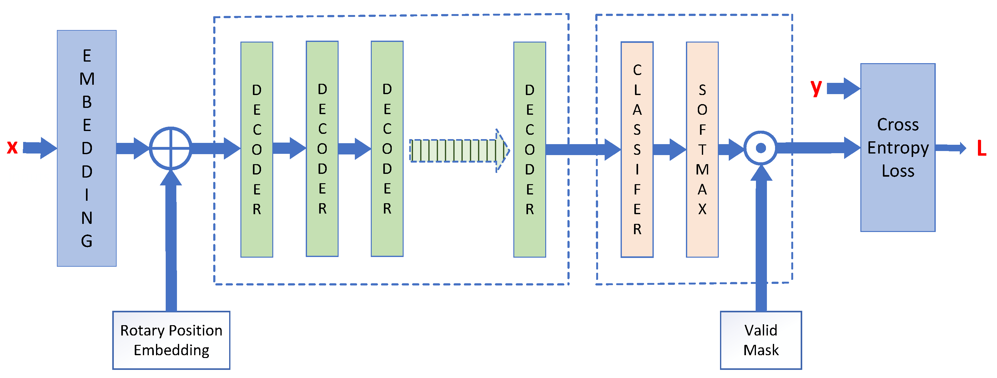
The Transformer architecture that we use for TSP optimization is shown in Figure 1. It is a Decoder-only architecture, as followed in many current LLM designs. There are two changes in our architecture with respect to a standard LLM Transformer. First is the difference in the embedding layer. In our design, the input is a sequence of node vectors (as opposed to tokens) and a potential near-optimal solution vector, as indicated in Equation (11). Thus, the embedding layer used is a simple linear layer with $2n+1$ inputs and d outputs, where d is the embedding dimensionality of the Transformer.

The second main change in our design is a Hadamard product of the “valid mask” with the output of the final softmax layer. In autoregressive generation, since the Transformer predicts the next node to visit (one at a time), the already-visited nodes should be removed from the set of remaining candidate nodes. We accommodate this by adding a mask entry at the position of the last-generated node number. Figure 2 shows the Decoder architecture. This is similar to an LLM Transformer Decoder.

4.4. Training and Generation for TSP Optimization

We follow a two-step approach to train the Transformer architecture for TSP optimization, as is followed in LLMs. The first step trains the architecture in a next-node prediction style by masking the future nodes. The training input is described by Equation (12):

$$n_0,n_1,\dots n_n,n_0,{\mathbf{n}}_{\mathbf{a}},{\mathbf{n}}_{\mathbf{b}},\dots ,{\mathbf{n}}_{\mathbf{0}}$$

(12)

The bold part in Equation (12) is the target near-optimal sequence. The bold parts are masked out, one at a time, during the next-node prediction training process. As an example, for the input $n_0,n_1,\dots n_n,n_0$, the target node is ${\mathbf{n}}_{\mathbf{a}}$. Similarly, for the input node sequence $n_0,n_1,\dots n_n,n_0,n_a$, the predicted node is ${\mathbf{n}}_{\mathbf{b}}$, and in the same manner onward. The implementation uses triangular masked attention in the target sequence part to speed up training. From a randomly generated dataset of TSP graphs and their near-optimal solutions, the Transformer architecture is trained using the cross-entropy loss, with “valid mask” to guarantee that the Hamiltonian cycle it learns is valid. The predicted node $\widehat{n_i}$ is determined as given in Equation (13):

$$\widehat{n_i}=\underset{i}{argmax}[softmax\left(classifier(L_{k-1}\left(L_{k-2}(\dots L_0(embedding\left(x\right)+PE\left(x\right)))\right)\times Vali{d}_{mask})\right]$$

(13)

The valid mask zeros out the output from the final softmax layer for the position where the last node number was predicted. This eliminates the possibility of a duplicate node in the predicted tour. The cross-entropy loss used in training in the first step is described in Equation (14):

$$L\left(\theta \right)=-{\displaystyle \frac{1}{n}}\sum _{i=n}^{2n+1}\sum _{k\in N}{n}_{i,k}\log {\widehat{n}}_{i,k}$$

(14)

where n is the number of nodes in the graph, N is the set of nodes, and the subscript i indicates the position of the node in the output tour.

The second step of the training uses Reinforcement Learning (RL) to further improve the prediction capabilities for the TSP tour. We implement both the Proximal Policy Optimization (PPO) and the Direct Preference Optimization (DPO) algorithms that are popular in LLM training phases (RLHF). The DPO algorithm is more appropriate for TSP node prediction, as the preference between two generated tours can be exactly computed according to their tour cost without any need for human feedback. The DPO loss function given below in our implementation is from [35].

$${\mathcal{L}}_{DPO}({\pi }_{\theta };{\pi }_{ref})=-{\mathbb{E}}_{(x,y_w,y_l)\sim \mathcal{D}}\left[\log \sigma \left(\beta \log {\displaystyle \frac{{\pi }_{\theta }\left(y_w\right|x)}{{\pi }_{ref}\left(y_w\right|x)}}-\beta \log {\displaystyle \frac{{\pi }_{\theta }\left(y_l\right|x)}{{\pi }_{ref}\left(y_l\right|x)}}\right)\right]$$

(15)

DPO uses the model trained from the first step as the reference model $\left({\pi }_{ref}\right)$, and then tries to improve this via the preference data. The model that is being improved is referred to as $\left({\pi }_{\theta }\right)$. The winning response, i.e., $\left(y_w\right|x)$, is the preferred response, while $\left(y_l\right|x)$ is the non-preferred response. In TSP, preference data can be the near-optimal tour from training data, while the actual model output can be used as the non-preferred data in the preference pair, as it is higher cost. The DPO loss function as described above helps the model to improve its learning by favoring preferred responses while also keeping the model’s policy within reasonable bounds set by the reference model (i.e., the model that was trained in the first step).

Once the Transformer model has been trained in a two-step process as described above, it can be used to generate the near-optimal tour by feeding it the sequence of nodes in the format described by Equation (11). The target sequence component in this sequence is changed to all nodes being the zero node. Starting from the sequence of given nodes in the graph and node 0, the model predicts the first node in the tour that follows node 0. This predicted node is then appended to the input sequence after node 0, and the next node is predicted. Valid masking is used so that a previously predicted node cannot be predicted. This autoregressive process is repeated until the complete tour is generated, returning to node 0.

5. Results

We generated TSP training data for many randomly generated graphs between 20 and 100 nodes. The random graphs were then optimized in a near-optimal manner using the parallel ACO TSP solver presented in [12]. The original graph and its near-optimal solution were then combined to generate the training data for the TSP Transformer architecture as described in the previous section. We compared the results on a test set of 10 randomly generated graphs for the following cases:

• Using only step 1 of training, where the model is trained for next-node prediction based on the cross-entropy loss only (referred to as CET—cross-entropy training);
• Using only step 2 of training, where the model is trained for tour prediction using a DPO loss only (referred to as DPOT—i.e., DPO training);
• Using both step 1 and step 2 where the model is trained using both cross-entropy loss and DPO loss (referred to as CET–DPOT).

The “% Optimal” numbers in

Table 1. Comparison of average test accuracy using cross-entropy and DPO for 10,000 and 50,000 training datapoints for different-sized TSP graphs.

Nodes	% Optimal 10,000 T. Data CET	% Optimal 10,000 T. Data DPOT	% Optimal 10,000 T. Data CET-DPOT	% Optimal 50,000 T. Data CET-DPOT
20	3.4	3.5	3.3	2.9
40	8.8	8.9	8.4	6.3
60	13.6	13.9	13.4	11.8
80	17.4	17.9	17.2	15.9
100	21.8	21.3	21.6	19.6

represent the tour cost within a percentage of the known optimal value. The test data are a set of randomly generated graphs that were not used in training the model. From Table 1, it can be seen that, while both loss functions individually are able to make the model learn effectively and peform a good prediction of the near-optimal tour, using both of these (as is typically followed in an LLM training) yields better results.

We also compare the percentage optimal results on the TSPLIB benchmarks for some of the graphs up to 100 nodes.

Table 2. Comparison of average test accuracy using cross-entropy and DPO for 10,000 and 50,000 training datapoints for different TSPLIB benchmarks.

TSPLIB Benchmark	Number of Nodes	% Optimal 10,000 T. Data CET	% Optimal 10,000 T. Data DPOT	% Optimal 10,000 T. Data CET-DPOT	% Optimal 50,000 T. Data CET-DPOT
Bays29	29	3.5	3.7	3.3	2.5
Berlin52	52	4.5	4.8	4.2	3.7
Eil76	76	7.8	8.1	7.6	5.6
KroA100	100	15.6	15.9	15.4	9.8
KroB100	100	17.1	17.7	17.7	10.1
KroC100	100	16.3	16.4	16.9	10.9
KroD100	100	19.8	19.9	18.8	12.9
KroE100	100	18.8	18.2	18.7	11.9

shows the results in terms of the percentage of the known optimal tour cost. As can be seen, more training data help the model to generalize effectively and produce better results.

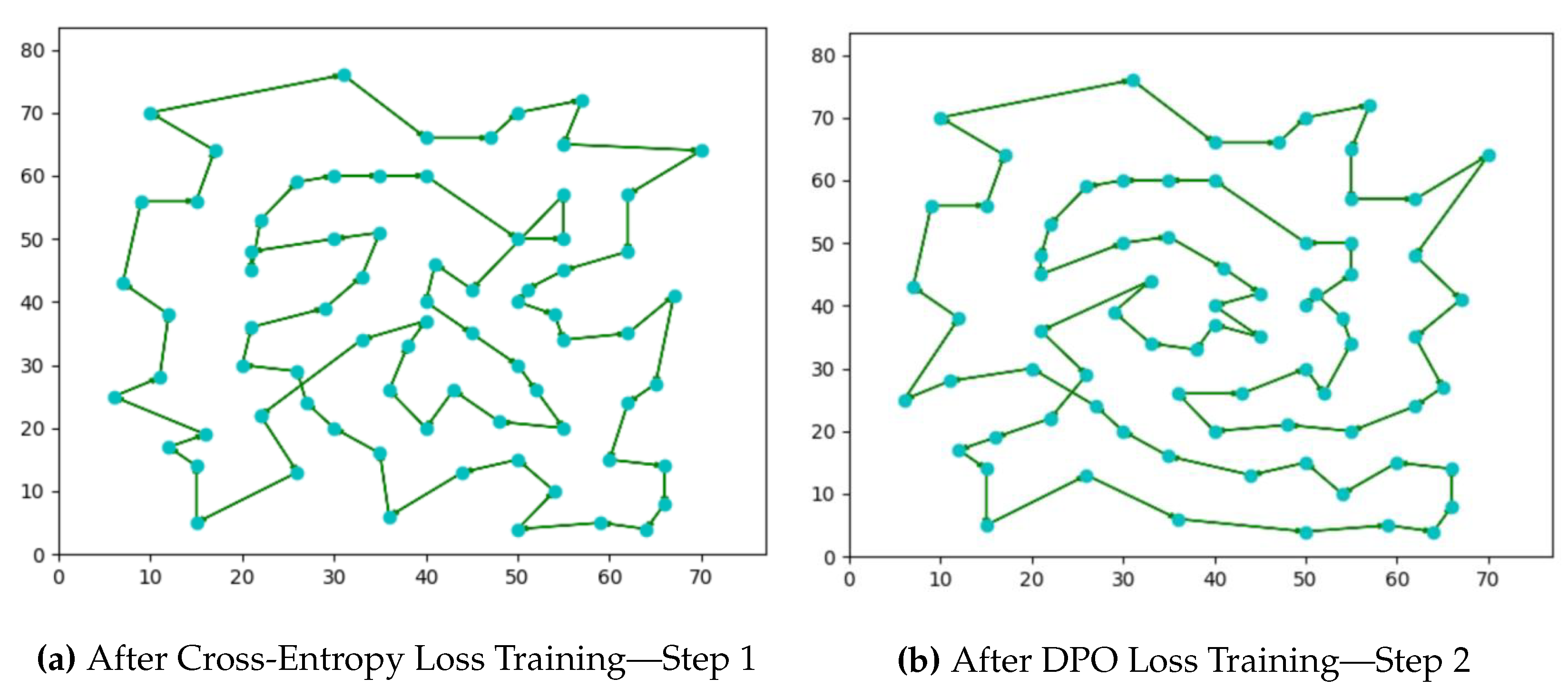
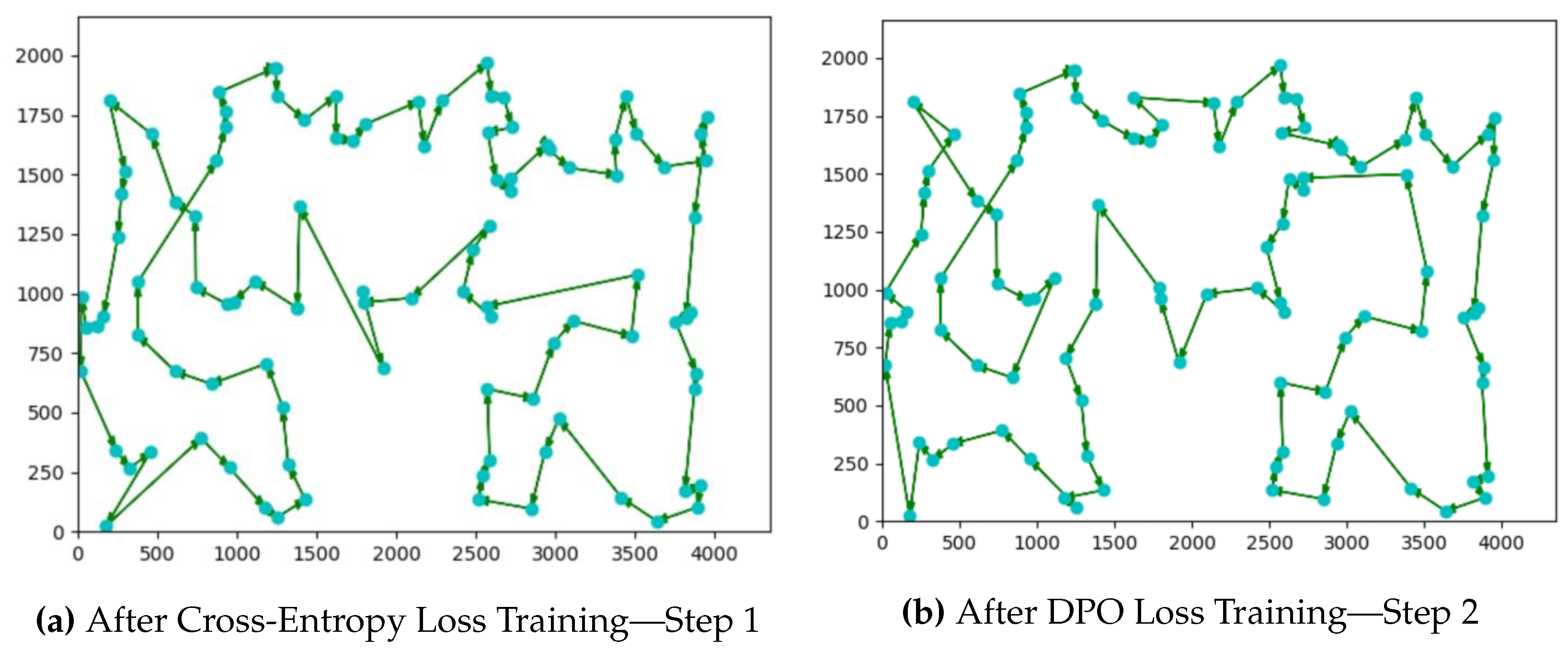
Figure 3, Figure 4 and Figure 5 show the actual tour generated by the trained TSP Transformer using both training steps of cross-entropy and DPO with 50,000 training datapoints. For smaller graphs, the results are closer to the optimal than compared to relatively larger node graphs. However, as more training data are used, the tour generation reaches closer to the optimal cost.

We also attempted to use the PPO algorithm in step 2 of the training. This did not produce an improvement over step 1 of the training process. However, the DPO algorithm is more effective and we used it in our results.

6. Discussion

From the results in the previous section, it is clear that the Transformer architecture is able to learn a near-optimal one-shot solution to the TSP optimization problem. The quality of the results improves as more training data are employed, as indicated in Table 1 and Table 2. The first step in training (via the cross-entropy loss) learns the conditional distribution of nodes based on the given graph and the partial tour. If $T\left(x\right)$ is the target data distribution and $Y\left(x\right)$ is the model’s predicted distribution, we can mathematically see the learning via the cross-entropy loss as

$$\mathrm{H}(T,Y)=-\sum _{x}T\left(x\right)\log Y\left(x\right)$$

(16)

$$\mathrm{H}(T,Y)=-\sum _{x}T\left(x\right)[\log T\left(x\right)+\log Y\left(x\right)-\log T\left(x\right)]$$

(17)

$$\mathrm{H}(T,Y)=-\sum _{x}T\left(x\right)\left[\log T\left(x\right)+\log {\displaystyle \frac{Y\left(x\right)}{T\left(x\right)}}\right]$$

(18)

$$\mathrm{H}(T,Y)=-\sum _{x}T\left(x\right)\log T\left(x\right)-\sum _{x}T\left(x\right)\log {\displaystyle \frac{Y\left(x\right)}{T\left(x\right)}}$$

(19)

$$\mathrm{H}(T,Y)=H\left(T\right)+D_{KL}\left(T\right|\left|Y\right)$$

(20)

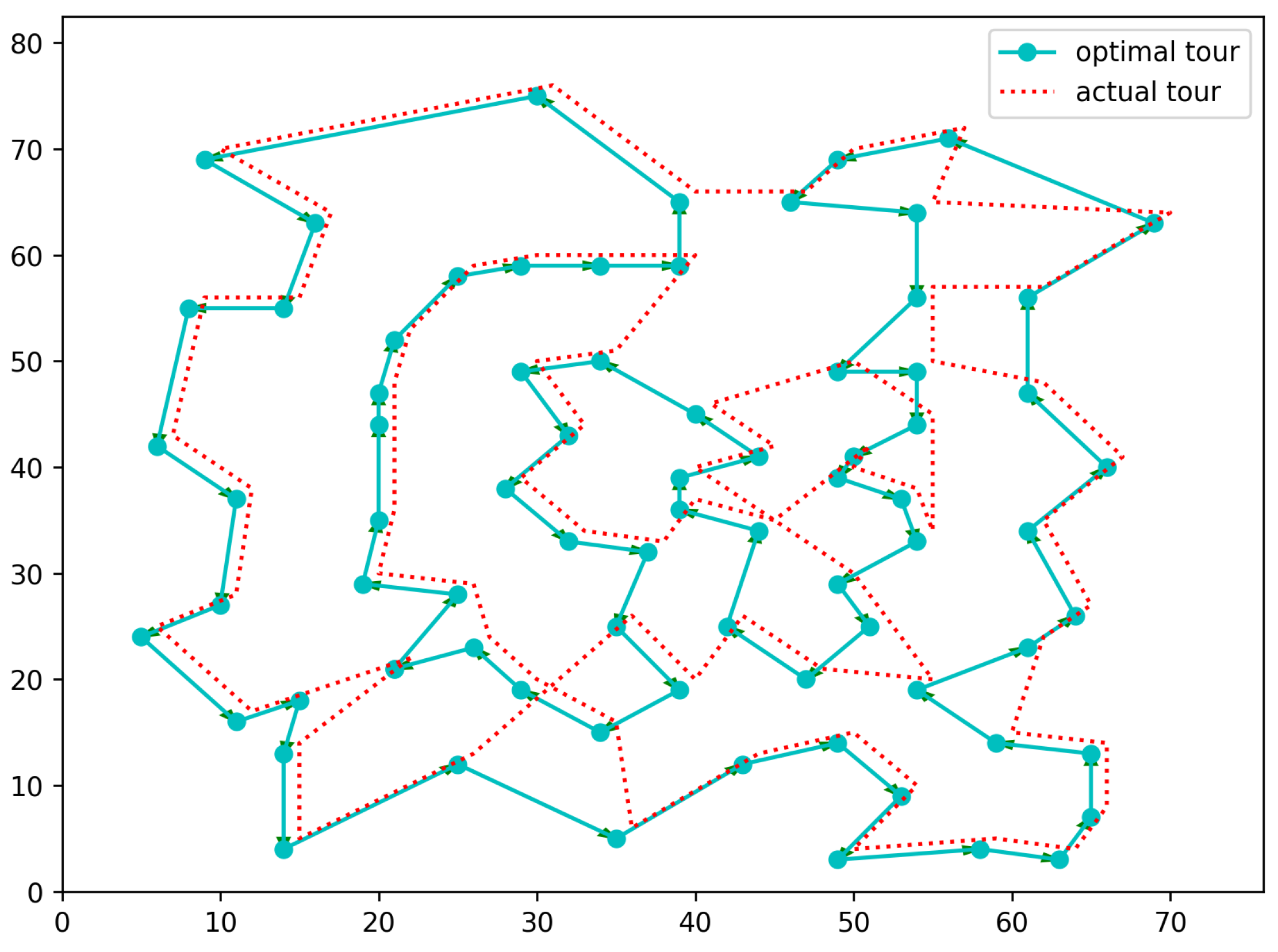
Since the target data distribution $T\left(x\right)$ is fixed, as can be seen from Equation (20), the model learns to reduce the $KL$ divergence between the learned distribution and the target data distribution as it minimizes the cross-entropy loss. This can be empirically observed from the results in the previous section, i.e., as more data are used, the model’s generalization improves. If we train the TSP Transformer on 100,000 training datapoints for 76 node randomly generated graphs and then test it on the Eil76 benchmark, the tour cost improves to 578 as opposed to 584, which was obtained with 50,000 training datapoints, as was shown in Figure 4. We show the improved generated tour for Eil76 in Figure 6 and also show how, for the majority of the tour, the learned model is following the optimal path, which it is learning via random graphs and their optimized solutions during training.

The second step of the training focuses on the entire tour. Using the Reinforcement Learning DPO algorithm, the quality of the generated tour (the entire tour) is optimized. Thus, the two-step training process in our implementation further improves the quality of optimization.

While we have demonstrated the effectiveness of our LLM-based learning approach to the one-shot solution of the TSP problem, our design can be easily adapted to some other NP-hard optimization problems, such as the Vehicle Routing Problem (VRP) and the Minimum Spanning Tree (MST) generation. In VRP, a given graph is the same as the TSP graph, the difference being that the tour generation covering all nodes is spanned by multiple vehicles, each having capacity and time window constraints. The constraints will need to be input as an additional set of tokens with the input graph. Similarly, in MST, the input graph is the same as TSP, but the generated output is the spanning tree, which is a subset of edges that connects all vertices without cycles with the minimum total edge weight. Thus, if training data with near-optimal solutions can be generated for VRP and MST, our LLM architecture can be easily adapted to these problem domains without causing any change in the training algorithms. The adaptation to a particular domain requires the change in the tokenization and the embedding vector format for each kind of optimization problem. In order to obtain good-quality optimal solutions, the challenge is in generating enough training data, especially for large-instance problems.

7. Conclusions

Our objective in this research was to explore the effective learning of LLM architecture and algorithms in the combinatorial optimization domain. We wanted to answer the following fundamental question: can the LLM designs learn to solve the NP-hard combinatorial optimization problem and provide a one-shot solution to the problem? To answer this, we adapt the ubiquitous LLM Transformer to the TSP optimization problem. The changes required in the LLM Transformer architecture are only at the input data level to the Transformer and an extra masking at the output to guarantee a valid Hamiltonian cycle in its generation.

The input data use a sequence of vectors, with each vector representing the node in the TSP graph and its relationship to other nodes. The rest of the Transformer architecture is kept the same as a canonical LLM Transformer, including its training regime in terms of next token generation via a cross-entropy loss, followed by Direct Preference Optimization, as followed in most LLMs.

Our results on both randomly generated graphs and TSPLIB benchmarks are very encouraging. With relatively small training data (≤50,000, whereas LLMs are trained on billions of datapoints), we are able to demonstrate the effective one-shot generation of the TSP optimization. The tour generated by the trained architecture has a cost < few% within the optimal cost for TSP graphs with up to 100 nodes. Note that this is a one-shot solution without any iterative refinement.

Our future work involves a more effective training of the architecture in terms of data quality, i.e., using more effective training data by examining in which cases it can be improved in its generalization. While we have seen considerable improvement in optimization by the use of the RL DPO algorithm, recently, an improved version of it, termed Tree Preference Optimization (TPO) [36], has been proposed. TPO formulates the language model alignment as a Preference List Ranking problem, where it learns more effectively from a ranked preference list of responses given the prompt. This is in contrast to simply a pair of responses, as used in DPO. Another possible improvement can be accomplished via a more effective, recently proposed Transformer architecture [37] that naturally suits to a fixed context, as in a given TSP graph, and has better learning comprehension for autoregressive generation. In addition, we plan to explore other constrained combinatorial optimization problems such as VRP and MST.

References

- Zuo, Y.; Qu, S.; Li, Y.; Chen, Z.; Zhu, X.; Hua, E.; Zhang, K.; Ding, N.; Zhou, B. MedXpertQA: Benchmarking Expert-Level Medical Reasoning and Understanding. arXiv 2025, arXiv:2501.18362. [Google Scholar]
- Karp, R.M. Reducibility among Combinatorial Problems. In Complexity of Computer Computations, Proceedings of a Symposium on the Complexity of Computer Computations, Yorktown Heights, NY, USA, 20–22 March 1972; Springer: New York, NY, USA, 1972; pp. 85–103. [Google Scholar]
- Larranaga, P.; Kuijpers, C.M.H.; Murga, R.H.; Inza, I.; Dizdarevic, S. Genetic Algorithms for the Travelling Salesman Problem: A Review of Representations and Operators. Artif. Intell. Rev. 1999, 13, 129–170. [Google Scholar]
- Razali, N.M.; Geraghty, J. Genetic Algorithm Performance with Different Selection Strategies in Solving TSP. In Proceedings of the World Congress on Engineering 2011, London, UK, 6–8 July 2011; International Association of Engineers: Hong Kong, China, 2011; Volume 2, pp. 1–6. [Google Scholar]
- Ezugwu, A.E.-S.; Adewumi, A.O.; Frîncu, M.E. Simulated Annealing Based Symbiotic Organisms Search Optimization Algorithm for Traveling Salesman Problem. Expert Syst. Appl. 2017, 77, 189–210. [Google Scholar] [CrossRef]
- Meer, K. Simulated Annealing versus Metropolis for a TSP Instance. Inf. Process. Lett 2007, 104, 216–219. [Google Scholar] [CrossRef]
- Fiechter, C.-N. A Parallel Tabu Search Algorithm for Large Traveling Salesman Problems. Discret. Appl. Math 1994, 51, 243–267. [Google Scholar]
- Brandão, J. A Tabu Search Algorithm for the Open Vehicle Routing Problem. Eur. J. Oper. Res. 2004, 157, 552–564. [Google Scholar]
- Wang, K.-P.; Huang, L.; Zhou, C.-G.; Pang, W. Particle Swarm Optimization for Traveling Salesman Problem. In Proceedings of the 2003 International Conference on Machine Learning and Cybernetics, Xi’an, China, 5 November 2003; IEEE: Piscataway, NJ, USA, 2003; Volume 3, pp. 1583–1585. [Google Scholar]
- Lu, C.; Wang, Q.X. Particle Swarm Optimization-Based Algorithms for TSP and Generalized TSP. Inf. Process. Lett. 2007, 103, 169–176. [Google Scholar]
- Yang, J.; Shi, X.; Marchese, M.; Liang, Y. An Ant Colony Optimization Method for Generalized TSP Problem. Prog. Nat. Sci. 2008, 18, 1417–1422. [Google Scholar]
- Ghimire, B.; Cohen, D.; Mahmood, A. Parallel Cooperating Ant Colonies with Improved Periodic Exchange Strategies. In Proceedings of the High Performance Computing Symposium, Tampa, FL, USA, 13–16 April 2014; pp. 1–6. [Google Scholar]
- Merz, P.; Freisleben, B. Memetic Algorithms for the Traveling Salesman Problem. Complex Syst. 2001, 13, 297–346. [Google Scholar]
- Gutin, G.; Karapetyan, D. A Memetic Algorithm for the Generalized Traveling Salesman Problem. Nat. Comput. 2010, 9, 47–60. [Google Scholar]
- Mahi, M.; Baykan, Ö.K.; Kodaz, H. A New Hybrid Method Based on Particle Swarm Optimization, Ant Colony Optimization and 3-opt Algorithms for Traveling Salesman Problem. Appl. Soft Comput. 2015, 30, 484–490. [Google Scholar] [CrossRef]
- Küçükoğlu, İ.; Dewil, R.; Cattrysse, D. Hybrid Simulated Annealing and Tabu Search Method for the Electric Travelling Salesman Problem with Time Windows and Mixed Charging Rates. Expert Syst. Appl. 2019, 134, 279–303. [Google Scholar] [CrossRef]
- Stützle, T. Parallelization Strategies for Ant Colony Optimization. In Proceedings of the International Conference on Parallel Problem Solving from Nature, Amsterdam, The Netherlands, 27–30 September 1998; Springer: Berlin/Heidelberg, Germany, 1998; pp. 722–731. [Google Scholar]
- Cantu-Paz, E.; Goldberg, D.E. Efficient Parallel Genetic Algorithms: Theory and Practice. Comput. Methods Appl. Mech. Eng. 2000, 186, 221–238. [Google Scholar]
- Vinyals, O.; Fortunato, M.; Jaitly, N. Pointer Networks. Adv. Neural Inf. Process. Syst. 2015, 28, 2692–2700. [Google Scholar]
- Bello, I.; Pham, H.; Le, Q.V.; Norouzi, M.; Bengio, S. Neural Combinatorial Optimization with Reinforcement Learning. arXiv 2016, arXiv:1611.09940. [Google Scholar]
- Prates, M.; Avelar, P.H.C.; Lemos, H.; Lamb, L.C.; Vardi, M.Y. Learning to Solve NP-Complete Problems: A Graph Neural Network for Decision TSP. Proc. AAAI Conf. Artif. Intell. 2019, 33, 4731–4738. [Google Scholar] [CrossRef]
- Hu, Y.; Zhang, Z.; Yao, Y.; Huyan, X.; Zhou, X.; Lee, W.S. A Bidirectional Graph Neural Network for Traveling Salesman Problems on Arbitrary Symmetric Graphs. Eng. Appl. Artif. Intell. 2021, 97, 104061. [Google Scholar]
- Vaswani, A. Attention Is All You Need. Adv. Neural Inf. Process. Syst. 2017, 30, 5998–6008. [Google Scholar]
- Dosovitskiy, A.; Beyer, L.; Kolesnikov, A.; Weissenborn, D.; Zhai, X.; Unterthiner, T.; Dehghani, M.; Minderer, M.; Heigold, G.; Gelly, S.; et al. An Image is Worth 16x16 Words: Transformers for Image Recognition at Scale. arXiv 2020, arXiv:2010.11929. [Google Scholar]
- Mahmood, K.; Mahmood, R.; Van Dijk, M. On the Robustness of Vision Transformers to Adversarial Examples. In Proceedings of the IEEE/CVF International Conference on Computer Vision, Online, 11–17 October 2021; pp. 7838–7847. [Google Scholar]
- Bresson, X.; Laurent, T. The Transformer Network for the Traveling Salesman Problem. arXiv 2021, arXiv:2103.03012. [Google Scholar]
- Pan, X.; Jin, Y.; Ding, Y.; Feng, M.; Zhao, L.; Song, L.; Bian, J. H-TSP: Hierarchically Solving the Large-Scale Traveling Salesman Problem. Proc. AAAI Conf. Artif. Intell. 2023, 37, 9345–9353. [Google Scholar] [CrossRef]
- Luo, F.; Lin, X.; Liu, F.; Zhang, Q.; Wang, Z. Neural Combinatorial Optimization with Heavy Decoder: Toward Large Scale Generalization. Adv. Neural Inf. Process. Syst. 2023, 36, 8845–8864. [Google Scholar]
- Ye, H.; Wang, J.; Cao, Z.; Berto, F.; Hua, C.; Kim, H.; Park, J.; Song, G. Large Language Models as Hyper-Heuristics for Combinatorial Optimization. arXiv 2024, arXiv:2402.01145. [Google Scholar]
- Schulman, J.; Wolski, F.; Dhariwal, P.; Radford, A.; Klimov, O. Proximal policy optimization algorithms. arXiv 2017, arXiv:1707.06347. [Google Scholar]
- Ouyang, L.; Wu, J.; Jiang, X.; Almeida, D.; Wainwright, C.; Mishkin, P.; Zhang, C.; Agarwal, S.; Slama, K.; Ray, A.; et al. Training language models to follow instructions with human feedback. Adv. Neural Inf. Process. Syst. 2022, 35, 27730–27744. [Google Scholar]
- Shao, Z.; Wang, P.; Zhu, Q.; Xu, R.; Song, J.; Bi, X.; Zhang, H.; Zhang, M.; Li, Y.K.; Wu, Y.; et al. Deepseekmath: Pushing the limits of mathematical reasoning in open language models. arXiv 2024, arXiv:2402.03300. [Google Scholar]
- Dubey, A.; Jauhri, A.; Pandey, A.; Kadian, A.; Al-Dahle, A.; Letman, A.; Mathur, A.; Schelten, A.; Yang, A.; Fan, A.; et al. The llama 3 herd of models. arXiv 2024, arXiv:2407.21783. [Google Scholar]
- Liu, A.; Feng, B.; Xue, B.; Wang, B.; Wu, B.; Lu, C.; Zhao, C.; Deng, C.; Zhang, C.; Ruan, C.; et al. Deepseek-v3 technical report. arXiv 2024, arXiv:2412.19437. [Google Scholar]
- Rafailov, R.; Sharma, A.; Mitchell, E.; Manning, C.D.; Ermon, S.; Finn, C. Direct preference optimization: Your language model is secretly a reward model. Adv. Neural Inf. Process. Syst. 2024, 36, 53728–53741. [Google Scholar]
- Liao, W.; Chu, X.; Wang, Y. TPO: Aligning Large Language Models with Multi-branch & Multi-step Preference Trees. In Proceedings of the Thirteenth International Conference on Learning Representations, Singapore, 24–28 April 2025. [Google Scholar]
- Mahmood, K.; Huang, S. Enhanced Computationally Efficient Long LoRA Inspired Perceiver Architectures for Auto-Regressive Language Modeling. arXiv 2024, arXiv:2412.06106. [Google Scholar]