Article

Learning and Reconstruction of Mobile Robot Trajectories with LSTM Autoencoders: A Data-Driven Framework for Real-World Deployment

1
Department of Robotics, VSB—Technical University of Ostrava, 708 00 Ostrava, Czech Republic
2
Department of Control Systems and Instrumentation, VSB—Technical University of Ostrava, 708 00 Ostrava, Czech Republic
*
Authors to whom correspondence should be addressed.
AI 2025, 6(12), 302; https://doi.org/10.3390/ai6120302
Submission received: 29 September 2025 / Revised: 7 November 2025 / Accepted: 18 November 2025 / Published: 24 November 2025

Abstract

Accurate trajectory learning and reconstruction represent a core challenge in mobile robotics, particularly in environments affected by sensor noise, drift, and incomplete data. Addressing this challenge is essential for reliable navigation and motion control in real-world Internet of Robotic Things (IoRT) systems. This paper presents a data-driven framework for learning and reconstructing mobile robot trajectories using LSTM autoencoders. Trajectory data were collected from both simulation and real-world experiments with a Unitree GO1 quadruped robot, preprocessed through normalization, sequence padding, and trajectory boundary flags, and then used to train recurrent neural network models. The proposed architecture employs bidirectional LSTM layers and a custom loss function combining reconstruction, velocity, and boundary terms to improve trajectory stability. Experimental results show stable reconstruction accuracy across simulated and real-world datasets, with the position RMSE reduced from 0.92 m to 0.60 m and the yaw MAE improved from 0.49 rad to 0.17 rad on the most complex trajectory. The evaluation was conducted in controlled indoor conditions and offline mode, which defines the current scope of validation. Future work will extend the analysis to larger and more diverse environments and investigate extensions such as attention mechanisms, sensor fusion, and online learning to enhance adaptability in real-world deployment.

1. Introduction

The evolution of robotics, particularly through the integration of the Internet of Robotic Things (IoRT), marks a new era of technological innovation, where mobile robots operate within increasingly complex and dynamic environments. This convergence of robotic systems with IoT technologies enables enhanced communication and collaboration among autonomous agents, thereby improving operational efficiency across sectors such as logistics, healthcare, and manufacturing [1,2,3]. As robots navigate environments containing both static and dynamic obstacles, trajectory learning becomes a crucial capability for effective path planning, collision avoidance, and adaptive motion control [4]. Trajectory learning frameworks can also support 3D vision-based inspection tasks, such as a self-developed robot for structural crack damage recognition [5]. With the growing complexity of operational scenarios, the need for advanced trajectory learning methodologies has become increasingly evident [6,7,8]. By leveraging large datasets from varied operational contexts, trajectory learning enhances a robot’s situational awareness and adaptability, enabling safe and efficient navigation in intricate real-world settings [9,10,11]. Within IoRT systems, where overall performance depends on the seamless integration of heterogeneous data streams, trajectory learning plays a key role in improving the autonomy and intelligence of mobile robots [12,13,14,15]. In recent years, we have witnessed a profound impact of machine learning and deep neural networks on trajectory prediction and reconstruction. Recurrent neural networks (RNNs), particularly Long Short-Term Memory (LSTM) models, excel at capturing temporal dependencies in sequential data [16,17,18]. The integration of LSTMs with autoencoders has further advanced this field, providing robust mechanisms for dimensionality reduction and feature extraction, thereby enabling accurate trajectory reconstructions [19]. Enhancements such as attention mechanisms and hybrid architectures have significantly improved trajectory prediction performance [20,21,22]. In parallel, combining deep learning models with probabilistic estimators such as Kalman filters has proven effective in mitigating sensor-related uncertainty and improving temporal stability [23,24]. These trends collectively highlight the rapid evolution of data-driven approaches for motion prediction yet underline the persistent trade-off between model complexity, computational cost, and deployability in real-world robotic systems. Despite these advances, several challenges persist. Mobile robot trajectories are often affected by sensor noise, calibration errors, and drift, which lead to degraded position estimates and unstable predictions [25,26,27]. Data incompleteness further complicates the learning process, as missing or corrupted sensor readings reduce reconstruction reliability. Many state-of-the-art architectures require significant computational resources, making their deployment on embedded robotic platforms difficult without hardware acceleration or model compression techniques. The high computational demands also restrict their use in real-time or embedded robotic systems, where a balance between prediction accuracy and inference speed is critical. Thus, there is a clear motivation to develop lightweight models that retain accuracy and robustness under noisy and resource-constrained conditions. Developing models that maintain accuracy and stability while being deployable on resource-limited platforms remains an open research challenge. To address these challenges, this study investigates how data-driven sequence learning models can effectively represent and reconstruct robotic trajectories under realistic sensing and computational constraints. Specifically, we explore whether recurrent architectures such as LSTM autoencoders can overcome the trade-off between model complexity, temporal accuracy, and deployability in real-world robotics. Based on this motivation, we propose an LSTM autoencoder framework that integrates a custom loss function combining reconstruction, velocity, and boundary terms to enhance stability and dynamic consistency. The method introduces a complete data preprocessing-to-learning pipeline and demonstrates that the proposed approach can accurately reconstruct and generalize trajectories across both simulated and real-world datasets. Unlike many existing deep models, the architecture is designed with real-world deployment in mind, balancing reconstruction accuracy with computational efficiency and establishing a robust foundation for future research on attention mechanisms, sensor fusion, and adaptive online learning in autonomous robotic systems.

2. Data Acquisition and Preprocessing

The trajectory learning experiments relied on data collected from a Unitree GO1 [28] quadruped robot equipped with onboard inertial measurement units (IMUs), joint encoders, and a depth camera, see Figure 1. The platform is extended with an NVIDIA Jetson Xavier NX [29] computing unit, which enabled local data processing and wireless communication. During movement tasks, in which it was manually guided by an operator, the robot continuously recorded its position, speed, orientation, and corresponding time stamps, thereby ensuring that both the spatial dynamics and the temporal development of the trajectory were captured. The recorded data were transmitted in real time via the Wi-Fi module of the Jetson, supporting 2.4 GHz and 5 GHz IEEE 802.11 standards [30]. The communication uses the MQTT protocol, which is lightweight and well-suited for IoT and robotic applications, ensuring efficient and low-latency data transfer to the cloud. Raw measurements were stored in CSV format on cloud platform, with each entry representing one time step and containing Cartesian position (x, y, z), linear velocity components, orientation (roll, pitch, yaw), and time information.
The raw trajectory data contains a total of 21 columns, each representing a distinct measurement or metadata field. For trajectory reconstruction, the most relevant information includes position, velocity, orientation, and precise timestamps, while other fields provide supplementary details useful for analyzing network connectivity and communication performance. The dataset can be categorized into three groups, as summarized in Table 1.
All experiments were conducted in the laboratory of the Department of Robotics, an open research and teaching space measuring approximately 30 × 30 m. The facility is primarily designed for education and experimental work in industrial and collaborative robotics and is equipped with multiple workstations featuring robots from various manufacturers, workbenches, and dedicated educational zones. Additional laboratory equipment includes safety barriers, protective structures, and measurement apparatus. The laboratory floor is smooth concrete, providing a uniform and stable surface for quadruped locomotion. Industrial robot workstations are enclosed within wire mesh safety cages, ensuring operator safety and simultaneously reducing the impact of physical obstacles on wireless signal propagation.
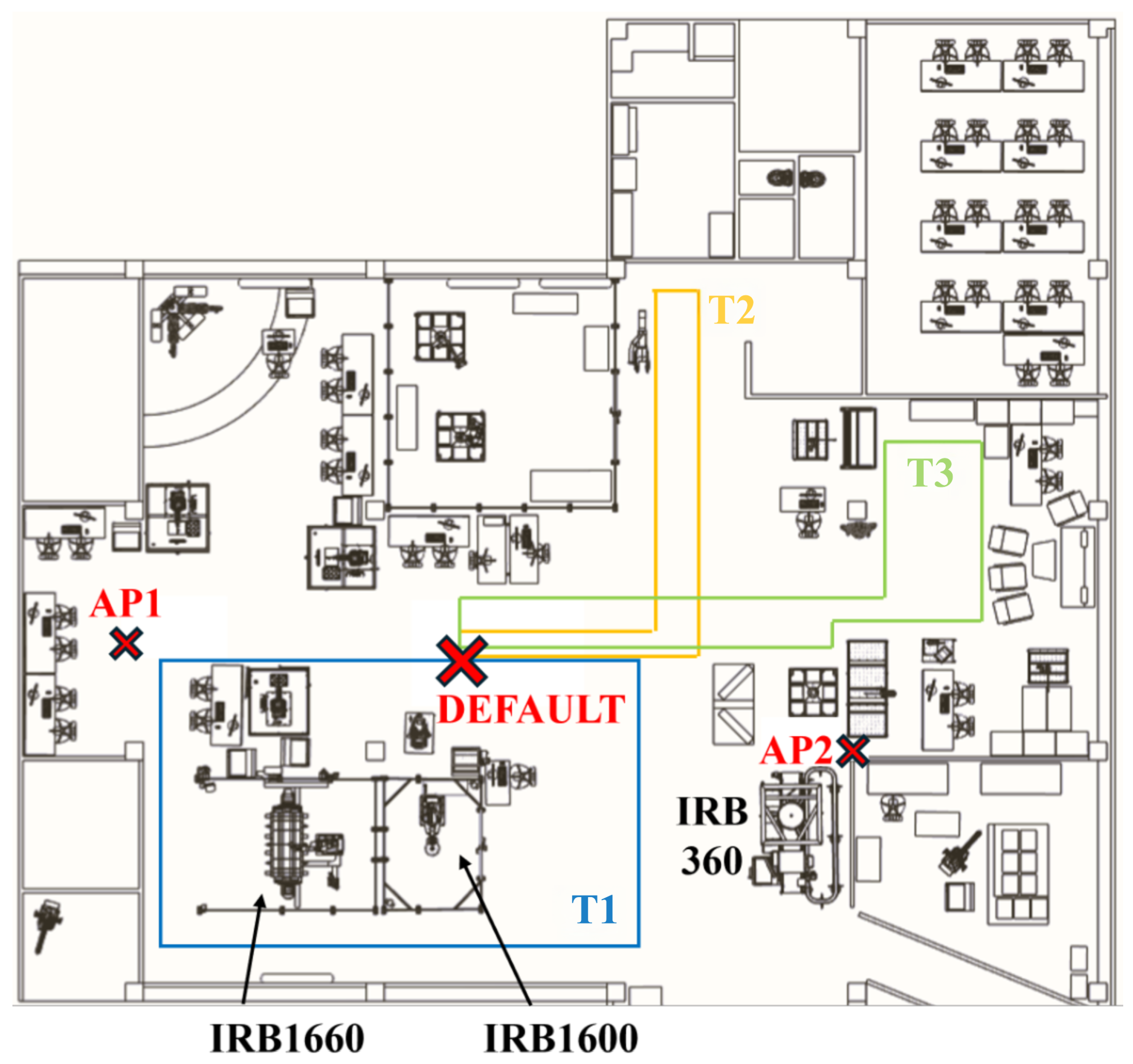
To evaluate the proposed method under different spatial and communication conditions, three distinct robot trajectories were designed within the laboratory environment. These paths are highlighted in Figure 2: T1 (blue), located in the western section of the facility near the ABB IRB1660 and IRB1600 industrial robots [31]; T2 (yellow), extending across the central corridor; and T3 (green), situated in the eastern part of the laboratory near IRB360 workstations. The routes were chosen to cover areas with varying wireless access point (AP1, AP2) coverage, obstacles, and workspace layouts, ensuring that the dataset captured heterogeneous conditions relevant for trajectory reconstruction and communication analysis.

3. LSTM Autoencoder Architecture

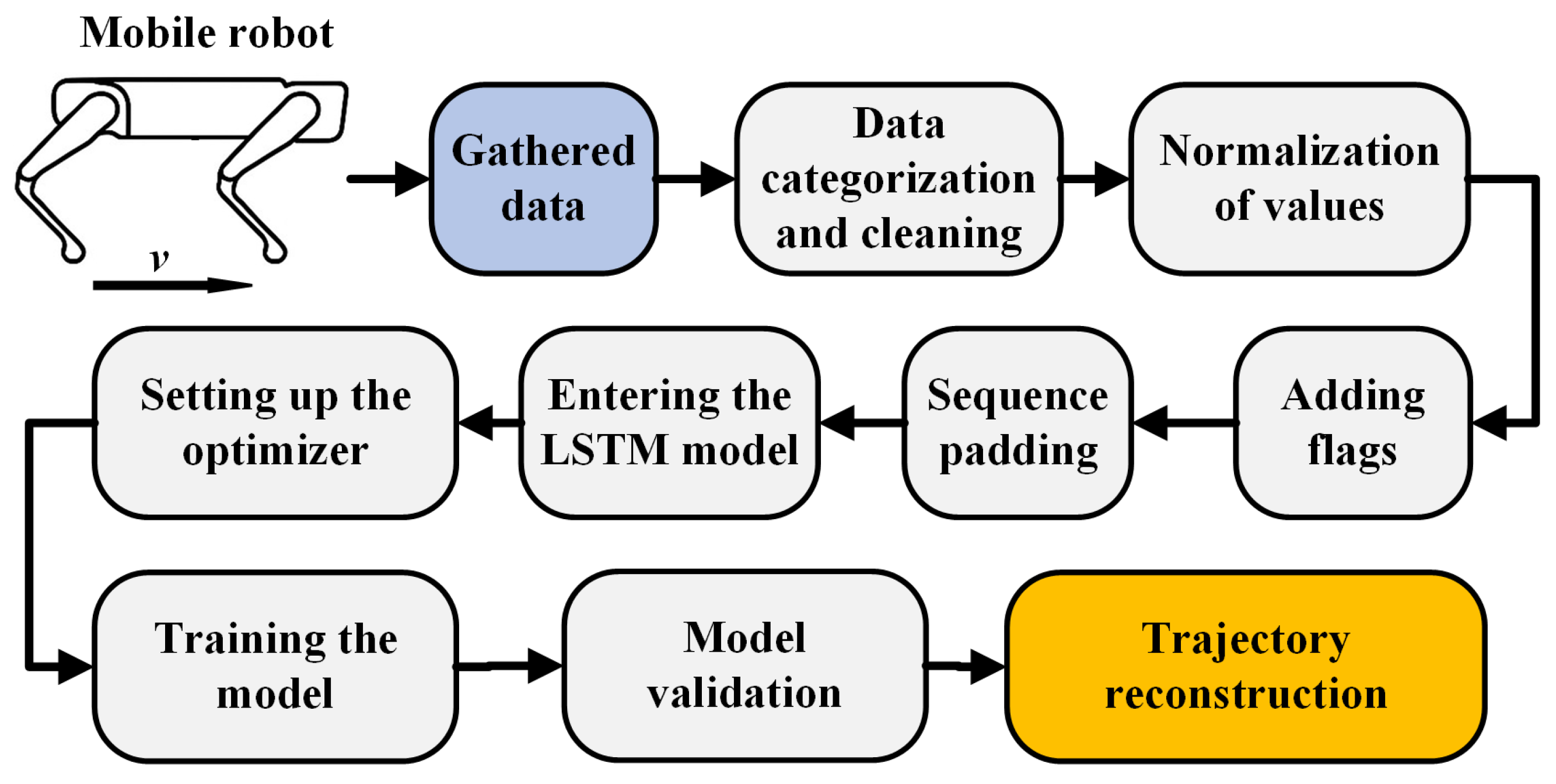
The proposed approach leverages a sequence-to-sequence deep learning model based on Long Short-Term Memory (LSTM) networks to learn and reconstruct robot trajectories. The method is designed to handle noisy and incomplete sensor data, ensuring stable trajectory generation in both simulated and real-world conditions. Figure 3 outlines the overall workflow, from data acquisition and preprocessing to model training, validation, and trajectory reconstruction.
Algorithm 1 outlines the procedure for loading and preprocessing trajectory data prior to training. First, relevant columns describing position, velocity, and orientation are extracted from the raw CSV files. The data are converted to numeric format, and corrupted entries are removed. Minimum and maximum values across all sequences are computed to enable global min–max normalization, ensuring consistency among trajectories. Additional binary flags are introduced to mark the start and end of each trajectory, which assist the LSTM autoencoder in recognizing sequence boundaries. The resulting sequences are stored as tensors together with their lengths. Finally, sequence padding is applied to standardize the input dimensions, and all preprocessed data are returned for subsequent training and validation.
The input data were normalized using a min–max transformation to scale all attributes into the range [0, 1]:
X = X X min X max X min + 10 8
where X denotes the original value of a given feature, X min and X max represent its minimum and maximum across the dataset, and X is the normalized value. Normalization was essential since the dataset contained attributes with different units and ranges (e.g., positions in meters, velocities in m/s, and orientation angles in radians). Without normalization, features with larger numerical ranges would dominate the training process, leading to unstable learning and poor generalization. By rescaling all values to a common interval, the neural network achieved more balanced weight updates, faster convergence, and reduced risk of vanishing or exploding gradients.
Since the neural network processes trajectories as sequences of time steps, it is important to explicitly mark the beginning and end of each trajectory. For this purpose, two binary flags were added:
  • Start_Flag—set to 1 for the first row of each trajectory, 0 otherwise.
  • End_Flag—set to 1 for the last row of each trajectory, 0 otherwise.
With these additional features, the input dimensionality expands from 7 to 9, where the original variables (Position_x, Position_y, Vel_Forward, Vel_Side, Roll, Pitch, Yaw) are complemented by Start_Flag and End_Flag. This information helps the network to better capture sequence boundaries and improves its ability to reconstruct transitions between trajectories.
Algorithm 1 Loading and preprocessing of trajectory data
  1:
Define selectedColumns ← {"Position_x", "Position_y", "Vel_Forward", "Vel_Side", "Roll", "Pitch", "Yaw"}
  2:
Initialize allData ← []
  3:
Initialize sequenceLengths ← []
  4:
Initialize minVals, maxVals ← None, None
  5:
Retrieve files ← all CSV files sorted in folderPath
  6:
for file in files do
  7:
      df ← Read CSV file with selectedColumns
  8:
      Convert df to numeric, remove NaN values
  9:
      if minVals is None then
10:
           minVals, maxVals ← Minimum and maximum values of df
11:
      else
12:
           Update minVals and maxVals using element-wise min/max
13:
      end if
14:
      Normalize df using: ( d f m i n V a l s ) / ( m a x V a l s m i n V a l s + 10 8 )
15:
      Add "Start_Flag" and "End_Flag" columns to df
16:
      Set first row "Start_Flag" ← 1, last row "End_Flag" ← 1
17:
      Append df as tensor to allData
18:
      Append len(df) to sequenceLengths
19:
end for
20:
Return allData, sequenceLengths, minVals, maxVals
21:
Load allData, sequenceLengths, minVals, maxVals ← load_data(folderPath)
22:
Apply padding: paddedSequencespad_sequence(allData)
23:
sequenceLengths ← Convert to tensor
As trajectories may vary in length depending on the measurement segment, a unification step was required before training. Recurrent neural networks such as LSTMs require input sequences within a batch to have the same length; therefore, padding was applied as follows:
  • The longest trajectory in the dataset defined the maximum sequence length.
  • Shorter trajectories were padded with zeros until they matched this length.
  • A masking mechanism was applied during training to ensure that padded values were ignored in loss computation and weight updates.
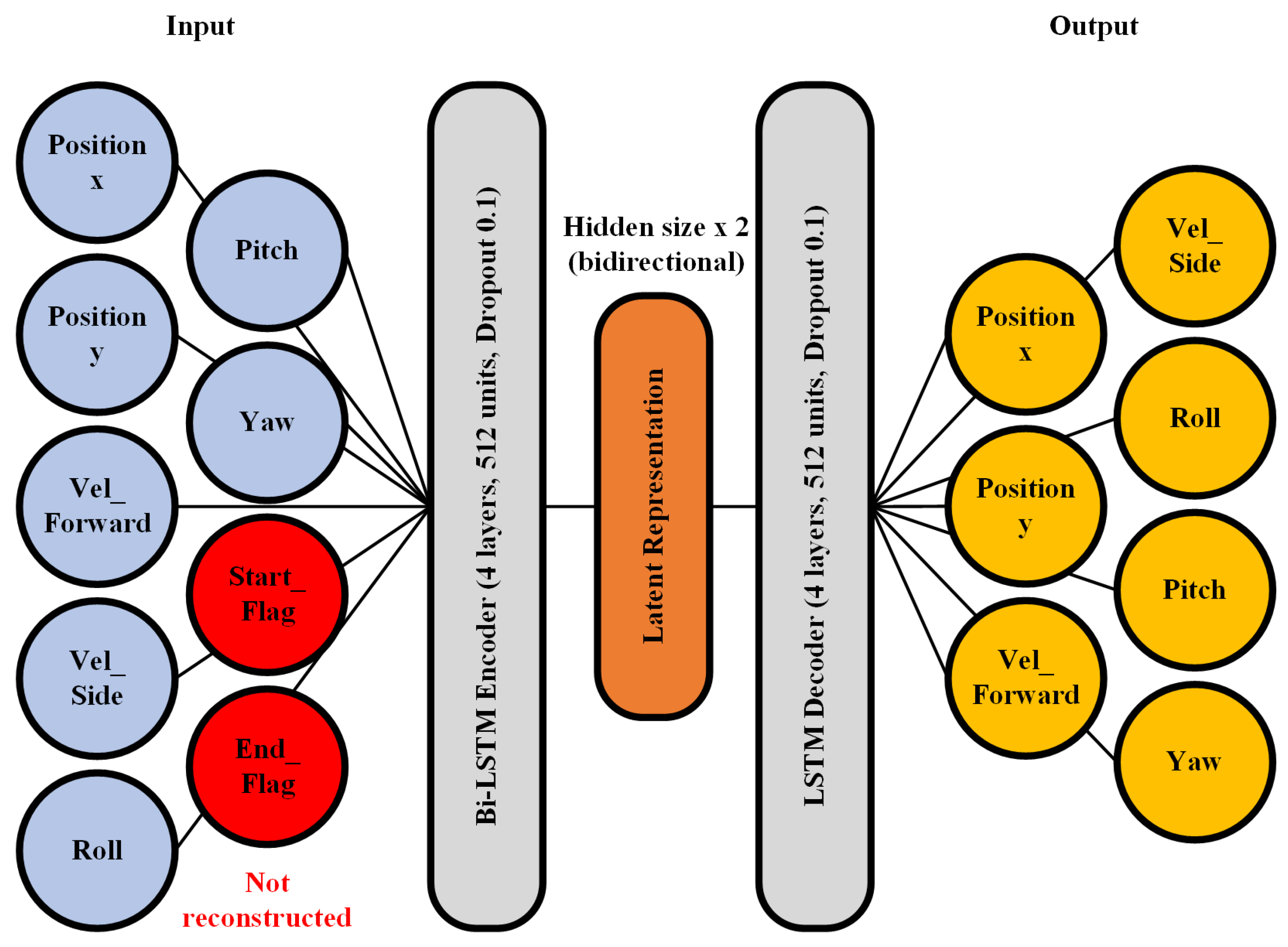
Algorithm 2 describes the training of the proposed LSTM autoencoder for trajectory reconstruction. The network processes sequences of position, velocity, and orientation, extended by two binary flags that mark the start and end of each trajectory. Its architecture consists of a bidirectional LSTM encoder, a multi-layer LSTM decoder, and a fully connected output layer (see Figure 4). The figure schematically shows the data flow through the proposed architecture. The encoder compresses each input trajectory sequence into a latent representation that captures its temporal structure, while the decoder reconstructs the original motion features from this representation. The inclusion of the Start and End flags and the composite loss terms is illustrated to emphasize how the network enforces smooth and consistent transitions between trajectory segments. With INPUT_SIZE = 9 and OUTPUT_SIZE = 7, the model learns to encode trajectories into a latent representation and decode them back to their original form. The hidden size of 512 units and four stacked layers allow the model to capture complex temporal dependencies, while dropout (0.1) reduces overfitting. Training is guided by a composite loss function that combines MSE and L1 reconstruction errors with velocity and boundary penalties, ensuring accurate and smooth trajectory reconstruction.
The total loss function used in Algorithm 2 for training is defined as:
L = L M S E + 0.7 L L 1 + 0.3 ( L s t a r t + L e n d ) + 0.2 L v e l
Here, L M S E ensures pointwise reconstruction accuracy, while L L 1 , weighted by 0.7, improves robustness against noise and outliers. The boundary losses L s t a r t and L e n d , weighted by 0.3, stabilize the trajectory at its beginning and end, and L v e l , weighted by 0.2, enforces motion smoothness through velocity consistency. The weights were empirically chosen to balance accuracy, stability, and smoothness, ensuring that the model reproduces trajectories while maintaining temporal coherence.
Algorithm 2 Training of the LSTM autoencoder for trajectory reconstruction
  1:
Define model parameters: INPUT_SIZE = 9, HIDDEN_SIZE = 512, NUM_LAYERS = 4, OUTPUT_SIZE = 7, DROPOUT = 0.1, Full-batch regime
  2:
Initialize bidirectional LSTM encoder, LSTM decoder, and fully connected output layer
  3:
Define loss functions: MSE, L1, velocity loss, and boundary loss
  4:
Initialize Adam optimizer with learning rate 0.0005 and weight decay 10 5
  5:
for each epoch in 1 600  do
  6:
      Forward pass with input sequences
  7:
      Mask padded values
  8:
      Compute:
  •     MSE and L1 reconstruction losses
  •     Velocity loss for smoothness
  •     Start/end point losses
  9:
      Combine into total loss:
L = L M S E + 0.7 L L 1 + 0.3 ( L s t a r t + L e n d ) + 0.2 L v e l
10:
      Backpropagate and update model parameters
11:
end for
12:
Return trained model
The sensitivity analysis is shown in Table 2 and evaluates the influence of weighting factors in the proposed loss formula. The parameters w L 1 and w boundary were systematically varied to investigate the influence of the L1 reconstruction term and the boundary alignment term on the model performance. The results show that slight changes in both weight factors have only a small effect on the accuracy of trajectory reconstruction. Increasing the boundary weight w boundary from 0 to 0.3–0.6 slightly improves the consistency of position and orientation, confirming the positive contribution of the start/end penalty term.

4. Experimental Results

The experimental evaluation is designed to verify the ability of the proposed LSTM autoencoder to reconstruct robot trajectories under various conditions. For this purpose, two complementary datasets were used. Simulation data, which provide a controlled environment for benchmarking the learning process, and real-world data, which reflect sensor noise, IMU drift, and environmental variability. By comparing the performance of these datasets, the experiments aim to not only assess the accuracy of reconstruction but also evaluate the robustness of the model and its ability to generalize when applied in realistic deployment scenarios.

4.1. Simulation Data

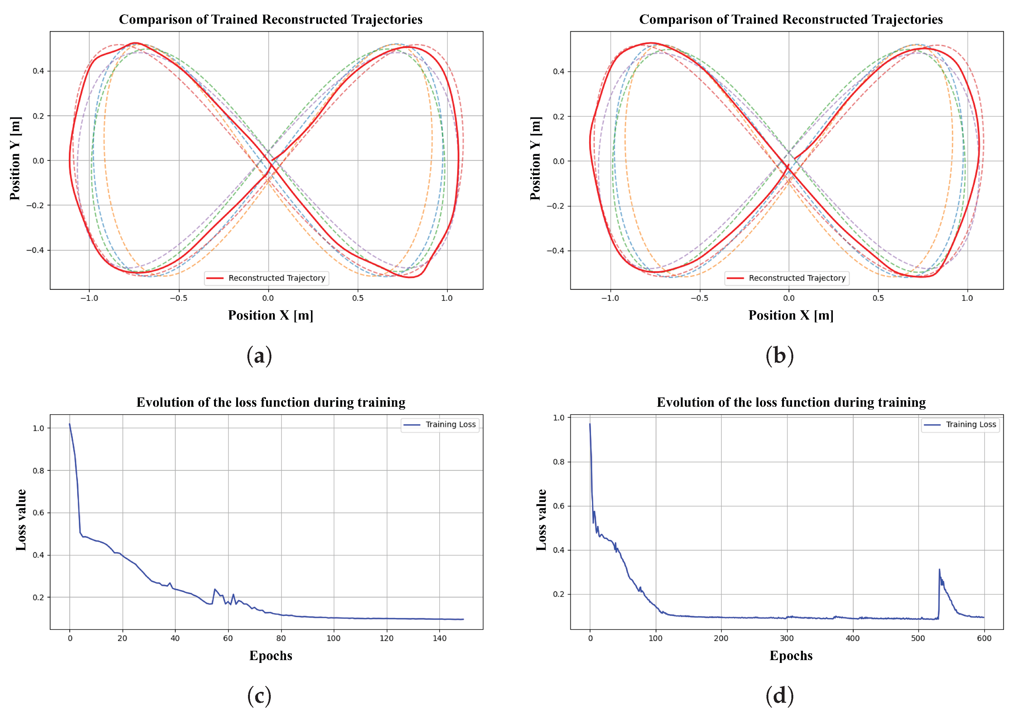
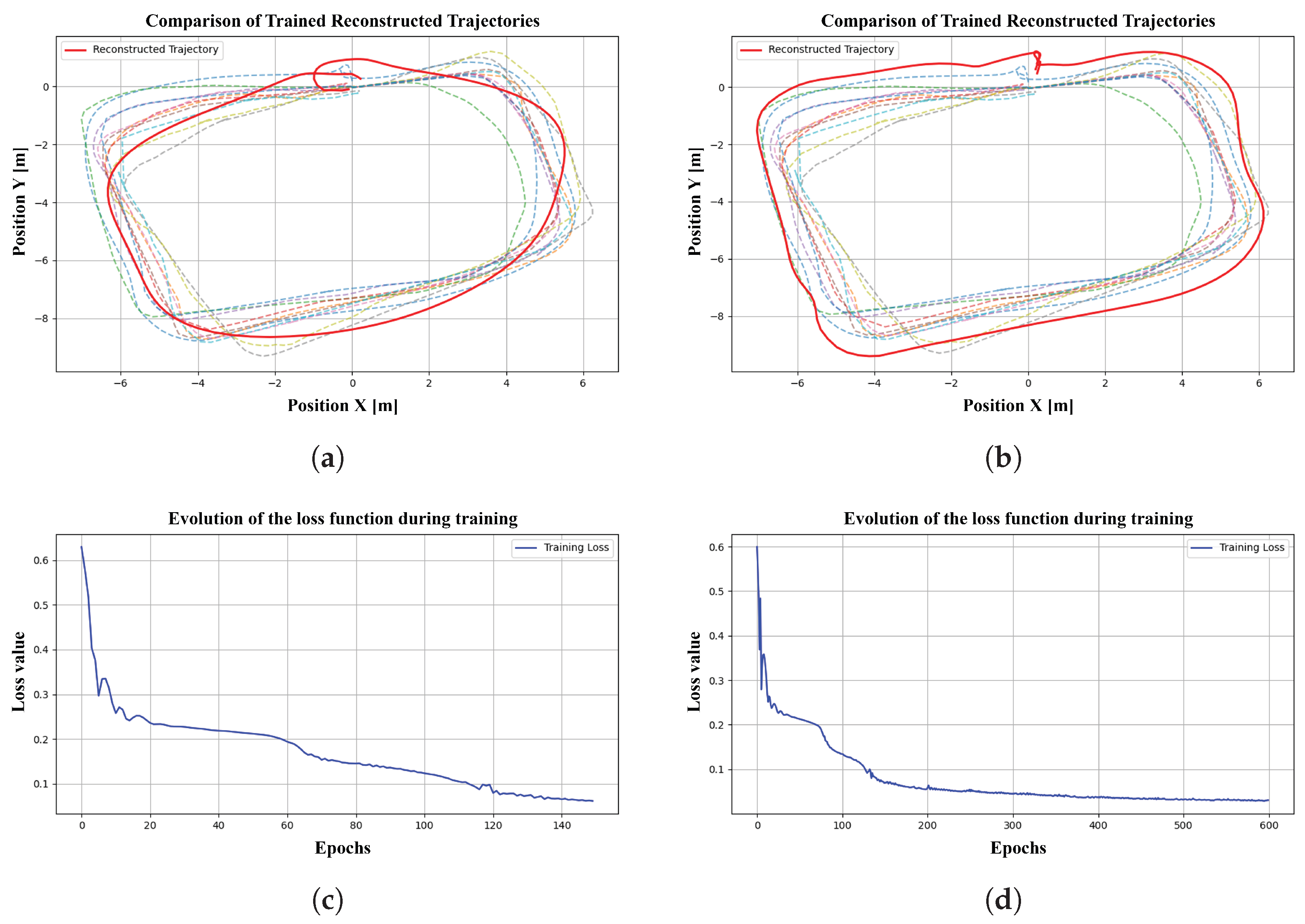
Artificial trajectories were designed to resemble typical robot movements, including straight paths, curves, and sudden directional changes. This controlled setup allowed the model to learn a wide range of motion patterns without the influence of sensor drift or terrain irregularities. Figure 5 illustrates reconstructed trajectories after 150 and 600 training epochs, respectively. The figure compares reconstructed trajectories with the original training data. After 150 epochs, the model captures the overall shape but shows minor deviations in curved segments. Extending training to 600 epochs results in smoother and more accurate reconstructions, with the figure-eight trajectory reproduced almost perfectly. The corresponding loss curves confirm this improvement: in both cases, the error drops rapidly at the beginning and stabilizes at a low value, with only minor fluctuations. A short increase around epoch 500 is observed but quickly subsides, indicating stable learning without signs of overfitting.

4.2. Real-World Data

The second part of the evaluation used trajectories measured directly from the Unitree GO1 robot in the laboratory. In contrast to simulation, these datasets include IMU drift, sensor noise, and environmental disturbances, making reconstruction more challenging and providing a realistic test of the model’s generalization capability.
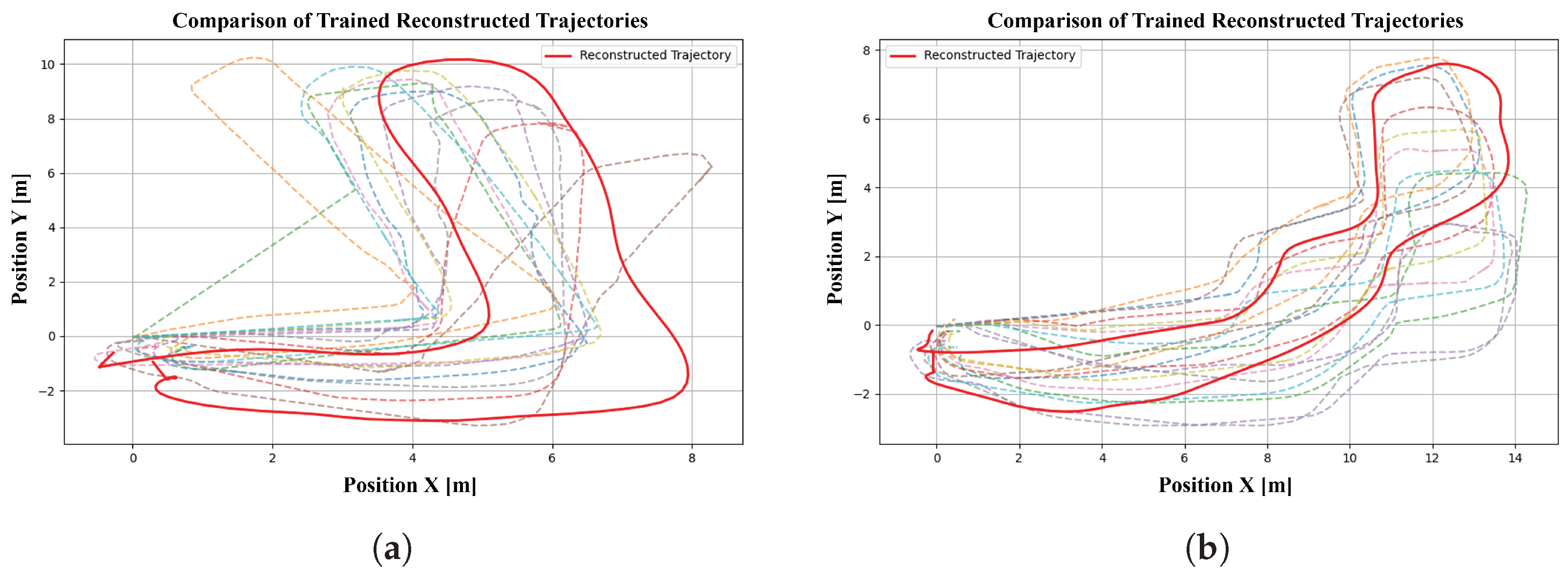
For trajectory T1, the model already captured the global shape after 150 epochs, with deviations in the upper section caused by drift (see Figure 6). After 600 epochs, the reconstruction was much more accurate, with the loss stabilizing slightly above 0.05 and the trajectory closely following the reference path. Trajectory T2 (see Figure 7a) represented a more complex motion with sharper turns. Here the model again converged stably. At 600 epochs, accuracy improved, though local details were partly smoothed, indicating the network’s tendency to average high-variability data. The most complex case, trajectory T3 (see Figure 7b), combined the largest data volume with frequent direction changes. Despite this, the model converged well, reducing the loss after 600 epochs. Reconstructions reproduced both the overall structure and finer curvature, though sharp transitions were still smoothed and drift effects persisted in long sections.
The evaluation on real-world data, recorded during the movement of the mobile robot with position estimates from an IMU, demonstrates that the model effectively learns to reconstruct trajectories. After 150 epochs, the training loss decreased rapidly from 0.6 to 0.07, with the reconstructed path largely following the training data but showing a notable deviation in the upper section caused by IMU drift. Extending training to 600 epochs further improved accuracy: the loss stabilized slightly above 0.05, and the reconstructed trajectory closely matched the reference data with only minor residual deformation. These results confirm that the model converges well and can partially compensate for sensor errors, although drift remains the main source of local distortion.
For the second trajectory (T2) on Figure 7, which represents a more complex motion sequence with greater variability in direction and shape, the model again demonstrated effective learning. After 150 epochs the loss dropped rapidly from above 0.6 to 0.1, indicating quick adaptation, while reconstruction still showed noticeable deviations in the upper sections, especially at sharp turns where IMU drift was most pronounced. After 600 epochs, the trajectory reconstruction became considerably more accurate and closely followed the training data, though the model tended to smooth finer details. This effect, common in data with high variability, suggests that more advanced architectures could further improve performance.
The third trajectory (T3) presented the most challenging scenario, with the highest data volume and the most complex motion patterns, including frequent changes of direction and speed. Despite this, the training remained stable, with the loss decreasing from 0.58 to 0.1 after 150 epochs and further to 0.06 after 600 epochs, without signs of overfitting. At 150 epochs, the model already reproduced the global structure but oversimplified complex segments. With extended training, the reconstructions improved significantly, better capturing curvature and local variations, though occasional smoothing at sharp transitions remained. IMU drift continued to affect long and intricate segments, but its impact was less severe than in T2. Quantitative metrics (see Table 3) were computed in Python 3.8 from synchronized trajectory pairs, where both reconstructed and reference sequences were truncated to the same length. Positional accuracy was evaluated using the RMSE and MAE over ( x , y ) coordinates, while the symmetric Hausdorff distance quantified the maximum spatial deviation. Velocity RMSE was calculated from forward and side velocity components, and yaw MAE expressed the orientation error in radians.
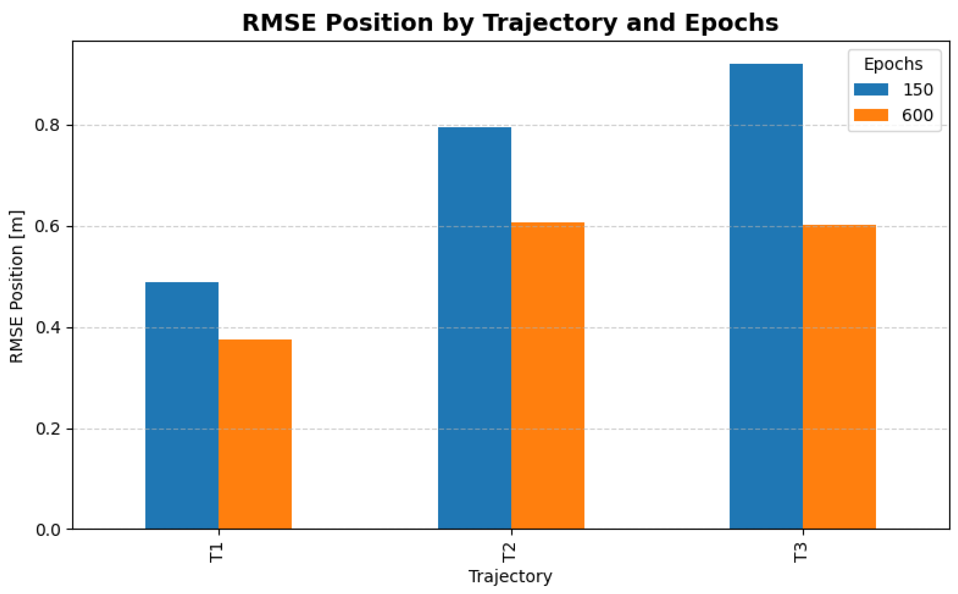
The quantitative evaluation summarized in Table 3 and visualized in Figure 8 shows that the proposed model achieves sub-meter reconstruction accuracy across all tested trajectories. For the simplest path (T1), the position RMSE decreased from 0.49 m after 150 epochs to 0.37 m after 600 epochs, accompanied by a reduction in maximum deviation (Hausdorff distance). For more complex trajectories (T2 and T3), the model preserved the overall shape but exhibited higher errors due to sharper turns and longer sequence lengths. In T3, however, extended training substantially improved performance, reducing the position RMSE from 0.92 m to 0.60 m and lowering the yaw error from 0.49 rad to 0.17 rad. Velocity errors remained relatively low in all cases (below 0.26 m/s), indicating that the reconstructed dynamics were consistent with the reference motion. These results demonstrate that the LSTM autoencoder can generalize to trajectories of different complexity, with longer training generally improving stability and orientation accuracy.
A quantitative comparison of the proposed LSTM autoencoder with established trajectory reconstruction methods is presented in Table 4. The results show that the proposed model provides the most balanced performance across all evaluated metrics, maintaining low positional and velocity errors while preserving orientation consistency. The Kalman filter achieved the lowest positional RMSE but exhibited higher velocity errors, indicating limited adaptability to nonlinear motion. The Transformer model demonstrated strong potential under dynamic conditions, with the lowest velocity and yaw errors, while the Seq2Seq-Attention network showed instability and reduced accuracy under the available data conditions. Overall, the results confirm the robustness and suitability of the proposed LSTM-based framework for reliable trajectory reconstruction in real-world deployment scenarios.

5. Discussion

During the course of this study, several important questions arose regarding the design, training, and evaluation of the proposed LSTM autoencoder for trajectory reconstruction. To better interpret the results and identify directions for further work, we address these questions in a structured discussion.
Q1: How does the proposed LSTM autoencoder relate to other sequence learning models?
The architecture was selected for its proven ability to capture temporal dependencies in trajectory data. Compared to traditional single-class SVM models and conventional autoencoders, the LSTM autoencoder has demonstrated its superiority in accurately recognizing data patterns in sequences, effectively reducing the number of false positives in scenarios such as web application breaches [32]. Furthermore, it is particularly well-suited for learning long-term dependencies in time series data, a fundamental aspect that distinguishes it from simpler recurrent neural networks (RNNs) and standard autoencoders, highlighting its usefulness in complex temporal tasks.
Q2: Can the learned representation be transferred across tasks or environments?
The study demonstrates successful generalization from simulation to real data. This points to the potential of reusing the learned latent representation for related tasks such as motion prediction, anomaly detection, or deployment on different robotic platforms. In particular, the proposed framework can be extended to wheeled or aerial robots, as its sequence-based design is not tied to a specific locomotion mechanism.
Q3: Does longer training always improve trajectory reconstruction?
Results suggest that additional training epochs significantly enhance accuracy and smoothness without clear signs of overfitting. However, marginal gains diminish after extended training, and occasional fluctuations in the loss indicate potential sensitivity to learning rate or data variability. Future versions of the framework should therefore incorporate explicit overfitting safeguards, such as learning rate scheduler.
Q4: What are the implications for online or real-time applications?
Although the evaluation was conducted offline, the compact model design and deployment on the Jetson platform indicate potential for future real-time implementation, which will be evaluated in subsequent work. Future work could extend this by analyzing and optimizing inference latency and exploring incremental learning strategies for online adaptation.
Q5: What role could trajectory autoencoders play beyond reconstruction?
Trajectory autoencoders have significant applications beyond reconstruction, particularly in anomaly detection and clustering. For instance, studies show that autoencoders trained on normal trajectory data can effectively identify anomalies by analyzing reconstruction errors—data samples with high reconstruction errors are flagged as anomalous, enhancing monitoring in fields such as traffic analysis and biological systems [33,34]. Moreover, by extracting meaningful features from high-dimensional trajectory data, autoencoders can improve clustering outcomes, allowing for more precise identification of movement patterns in complex datasets [35].
Furthermore, the evaluation of wireless network performance for the same robotic platform was carried out in our previous study [36], which provides a analysis of latency, packet loss, and communication reliability during robot motion.

6. Conclusions

This study introduced a trajectory reconstruction framework for mobile robots based on an LSTM autoencoder, supported by a complete preprocessing pipeline with normalization, sequence padding, and trajectory boundary flags. A custom loss function that combined reconstruction accuracy with velocity and boundary penalties was implemented to enhance trajectory stability.
Quantitative evaluation confirmed that the model consistently achieves mean positional RMSE below 0.6 m across all trajectories. For instance, in the most complex trajectory (T3), the position RMSE decreased by more than 34% and the yaw error by nearly 66% when extending training from 150 to 600 epochs. Velocity deviations remained low across all cases, indicating that the reconstructed dynamics closely matched the reference motion.
The findings indicate that LSTM autoencoders represent a reliable approach for trajectory reconstruction and provide a flexible basis for extending toward adaptive motion control, anomaly detection, and predictive planning in mobile robotics. Remaining limitations include sensitivity to IMU drift and the smoothing of sharp trajectory features, which could be mitigated through attention-based modeling, sensor fusion, or online adaptation methods.
While the proposed framework showed promising results, the experiments were limited to a controlled indoor environment and offline evaluation. Future research will therefore extend testing to environments of different scales and surface conditions, including outdoor settings, to further validate the model’s robustness and generalization. We also plan to extend the presented framework by integrating sensor fusion techniques to further mitigate IMU drift and measurement noise, enhancing trajectory stability in long-term deployments.

Author Contributions

Conceptualization, J.K. and M.B.; methodology, J.K.; validation, J.K. and M.B.; formal analysis, M.B.; investigation, J.K.; resources, J.K. and M.B.; data curation, M.B.; writing—original draft preparation, J.K.; writing—review and editing, J.K. and M.B.; visualization, J.K.; supervision, M.B.; project administration, V.K.; funding acquisition, Z.B. All authors have read and agreed to the published version of the manuscript.

Funding

This research was funded in part by by the European Union under the REFRESH—Research Excellence For REgion Sustainability and High-tech Industries project number CZ.10.03.01/ 00/22_003/0000048 via the Operational Programme Just Transition. This article was also supported by specific research projects SP2025/042, SP2025/006 and financed by the state budget of the Czech Republic.

Institutional Review Board Statement

Not applicable.

Informed Consent Statement

Not applicable.

Data Availability Statement

The data that supports the findings of this article is available from the corresponding authors upon reasonable request.

Acknowledgments

During the preparation of this work, the authors used Write-full (2025.66.0.), ChatGPT (version 5) and DeepL (version 5) in order to improve language and readability. After using this tool/service, the authors reviewed and edited the content as needed and take full responsibility for the content of the publication.

Conflicts of Interest

The authors declare no conflicts of interest.

Abbreviations

The following abbreviations are used in this manuscript:
IoRTInternet of Robotic Things
LSTMLong Short-Term Memory
RNNRecurrent Neural Network
IMUInertial Measurement Unit
CSVComma-Separated Values
MSEMean Squared Error
L1L1 Loss (Mean Absolute Error)
APAccess Point
MQTTMessage Queuing Telemetry Transport
MACMedium Access Control
PHYPhysical Layer
IEEEInstitute of Electrical and Electronics Engineers

References

  1. Molina-Leal, A.; Gómez-Espinosa, A.; Escobedo Cabello, J.A.; Cuan-Urquizo, E.; Cruz-Ramírez, S.R. Trajectory Planning for a Mobile Robot in a Dynamic Environment Using an LSTM Neural Network. Appl. Sci. 2021, 11, 10689. [Google Scholar] [CrossRef]
  2. Liu, H.; Bianchin, G.; Pasqualetti, F. Secure Trajectory Planning Against Undetectable Spoofing Attacks. Automatica 2020, 113, 108655. [Google Scholar] [CrossRef]
  3. Li, X.; Li, M. The direction analysis on trajectory of fast neural network learning robot. IEEE Access 2021, 9, 125580–125589. [Google Scholar] [CrossRef]
  4. Yang, L.; Li, P.; Qian, S.; He, Q.; Miao, J.; Liu, M.; Hu, Y.; Memetimin, E. Path planning technique for mobile robots: A review. Machines 2023, 11, 980. [Google Scholar] [CrossRef]
  5. Hu, K.; Chen, Z.; Kang, H.; Tang, Y. 3D vision technologies for a self-developed structural external crack damage recognition robot. Autom. Constr. 2024, 159, 105262. [Google Scholar] [CrossRef]
  6. Hoeller, D.; Wellhausen, L.; Farshidian, F.; Hutter, M. Learning a State Representation and Navigation in Cluttered and Dynamic Environments. IEEE Robot. Autom. Lett. 2021, 6, 1091–1098. [Google Scholar] [CrossRef]
  7. Altan, S.; Sarıel, I. CLUE-AI: A Convolutional Three-Stream Anomaly Identification Framework for Robot Manipulation. IEEE Access 2023, 11, 12763–12775. [Google Scholar] [CrossRef]
  8. Liang, Y. Robot trajectory tracking control based on neural networks and sliding mode control. IEEE Access 2025, 13, 96740–96757. [Google Scholar] [CrossRef]
  9. Azzam, R.; Taha, T.; Huang, S.; Zweiri, Y. A Deep Learning Framework for Robust Semantic SLAM. In Proceedings of the 2020 Advances in Science and Engineering Technology International Conferences (ASET), Dubai, United Arab Emirates, 4 February–9 April 2020; p. 9118181. [Google Scholar] [CrossRef]
  10. Keung, K.L.; Chow, K.H.; Lee, C. Collision avoidance and trajectory planning for autonomous mobile robot: A spatio-temporal deep learning approach. In Proceedings of the 2023 IEEE International Conference on Industrial Engineering and Engineering Management (IEEM), Singapore, 18–21 December 2023. [Google Scholar] [CrossRef]
  11. Dong, L.; He, Z.; Song, C.; Sun, C. A review of mobile robot motion planning methods: From classical motion planning workflows to reinforcement learning-based architectures. J. Syst. Eng. Electron. 2023, 34, 439–459. [Google Scholar] [CrossRef]
  12. Farajiparvar, P.; Ying, H.; Pandya, A. A brief survey of telerobotic time delay mitigation. Front. Robot. AI 2020, 7, 578805. [Google Scholar] [CrossRef] [PubMed]
  13. Wei, Y.; Jang-Jaccard, J.; Xu, W.; Sabrina, F.; Camtepe, S.; Boulic, M. Lstm-autoencoder based anomaly detection for indoor air quality time series data. arXiv 2022, arXiv:2204.06701. [Google Scholar] [CrossRef]
  14. Wei, S.; Lin, Y.; Wang, J.; Zeng, Y.; Qu, F.; Zhou, X.; Lu, Z. A robust tcphd filter for multi-sensor multitarget tracking based on a gaussian–student’s t-mixture model. Remote Sens. 2024, 16, 506. [Google Scholar] [CrossRef]
  15. Krish, V.; Mata, A.; Bak, S.; Hobbs, K.L.; Rahmati, A. Provable observation noise robustness for neural network control systems. Res. Dir.-Cyber-Phys. Syst. 2024, 2, e1. [Google Scholar] [CrossRef]
  16. Sarkar, M.; Ghose, D. Sequential learning of movement prediction in dynamic environments using lstm autoencoder. arXiv 2018, arXiv:1810.05394. [Google Scholar] [CrossRef]
  17. Chen, D.; Li, S.; Wu, Q. A novel supertwisting zeroing neural network with application to mobile robot manipulators. IEEE Trans. Neural Netw. Learn. Syst. 2021, 32, 1776–1787. [Google Scholar] [CrossRef]
  18. Samuel, R.D.J.; Cuzzolin, F. Unsupervised anomaly detection for a smart autonomous robotic assistant surgeon (saras) using a deep residual autoencoder. IEEE Robot. Autom. Lett. 2021, 6, 7256–7261. [Google Scholar] [CrossRef]
  19. Chirayil Nandakumar, S.; Mitchell, D.; Erden, M.S.; Flynn, D.; Lim, T. Anomaly Detection Methods in Autonomous Robotic Missions. Sensors 2024, 24, 1330. [Google Scholar] [CrossRef] [PubMed]
  20. Sünderhauf, N.; Brock, O.; Scheirer, W.; Hadsell, R.; Fox, D.; Leitner, J.; Upcroft, B.; Abbeel, P.; Burgard, W.; Milford, M.; et al. The Limits and Potentials of Deep Learning for Robotics. Int. J. Robot. Res. 2018, 37, 1053–1077. [Google Scholar] [CrossRef]
  21. Chen, R. Anomaly Detection Model Based on Anomaly Representation Reinforcement and Path Iterative Modeling. Concurr. Comput. Pract. Exp. 2025, 37, e70245. [Google Scholar] [CrossRef]
  22. Qin, W.; Tang, J.; Lu, C.; Lao, S. Trajectory prediction based on long short-term memory network and kalman filter using hurricanes as an example. Comput. Geosci. 2021, 25, 1005–1023. [Google Scholar] [CrossRef]
  23. Zheng, Y.; Xu, Y.; Lu, Z. Pedestrian Trajectory Prediction Based on LSTM-NMPC. Int. J. Automot. Eng. 2025, 13575, 1009–1016. [Google Scholar] [CrossRef]
  24. Woo, H.; Ji, Y.; Tamura, Y.; Kuroda, Y.; Sugano, T.; Yamamoto, Y.; Yamashita, A.; Asama, H. Trajectory prediction of surrounding vehicles considering individual driving characteristics. Int. J. Automot. Eng. 2018, 9, 282–288. [Google Scholar] [CrossRef] [PubMed]
  25. Shen, Y.; Zheng, J.; Ye, L.; El-Farra, N. Online Local Modeling and Prediction of Batch Process Trajectories Using Just-In-Time Learning and LSTM Neural Network. J. Comput. Methods Sci. Eng. 2020, 20, 611–624. [Google Scholar] [CrossRef]
  26. Tang, G.; Lei, J.; Shao, C.; Hu, X.; Cao, W.; Men, S. Short-term prediction in vessel heave motion based on improved lstm model. IEEE Access 2021, 9, 58067–58078. [Google Scholar] [CrossRef]
  27. Zhang, J.; Wang, H.; Cui, F.; Liu, Y.; Liu, Z.; Dong, J. Research into ship trajectory prediction based on an improved lstm network. J. Mar. Sci. Eng. 2023, 11, 1268. [Google Scholar] [CrossRef]
  28. Hangzhou Yushu Technology Co., Ltd. (Unitree Robotics). Unitree Go1: Bionic Companion Quadruped Robot. 2025. Available online: https://shop.unitree.com/products/unitreeyushutechnologydog-artificial-intelligence-companion-bionic-companion-intelligent-robot-go1-quadruped-robot-dog (accessed on 11 June 2025).
  29. NVIDIA Corporation. World’s Smallest AI Supercomputer: NVIDIA Jetson Xavier NX; NVIDIA Corporation: Santa Clara, CA, USA, 2025; Available online: https://www.nvidia.com/en-us/autonomous-machines/embedded-systems/jetson-xavier-nx/ (accessed on 11 June 2025).
  30. IEEE Std 802.11-2016; IEEE Standard for Information Technology—Telecommunications and Information Exchange Between Systems—Local and Metropolitan Area Networks—Specific Requirements—Part 11: Wireless LAN Medium Access Control (MAC) and Physical Layer (PHY) Specifications. Institute of Electrical and Electronics Engineers (IEEE): New York, NY, USA, 2016. Available online: https://standards.ieee.org/standard/802_11-2016.html (accessed on 5 June 2025).
  31. ABB. Industrial Robots; ABB Ltd.: Zürich, Switzerland, 2024; Available online: https://new.abb.com/products/robotics/cs/roboty/prumyslove-roboty (accessed on 5 June 2025).
  32. Shi, L.; Ma, Y.; Lü, Y.; Chen, L. The application of computer intelligence in the cyber-physical business system integration in network security. Comput. Intell. Neurosci. 2022, 2022, 5490779. [Google Scholar] [CrossRef]
  33. Li, C.; Feng, G.; Jia, Y.; Li, Y.; Ji, J.; Miao, Q. Retad. Int. J. Data Warehous. Min. 2023, 19, 1–14. [Google Scholar] [CrossRef]
  34. Lu, F.; Zhang, Z.; Shui, C. Online trajectory anomaly detection model based on graph neural networks and variational autoencoder. J. Phys. Conf. Ser. 2024, 2816, 012006. [Google Scholar] [CrossRef]
  35. Zeng, W.; Xu, Z.; Cai, Z.; Chu, X.; Lu, X. Aircraft trajectory clustering in terminal airspace based on deep autoencoder and gaussian mixture model. Aerospace 2021, 8, 266. [Google Scholar] [CrossRef]
  36. Krejčí, J.; Babiuch, M.; Suder, J.; Krys, V.; Bobovský, Z. Latency-Sensitive Wireless Communication in Dynamically Moving Robots for Urban Mobility Applications. Smart Cities 2025, 8, 105. [Google Scholar] [CrossRef]
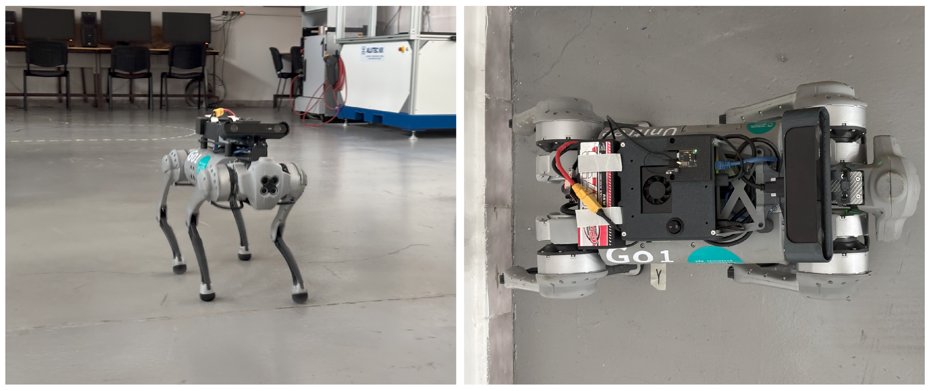
Figure 1. Unitree GO1 quadruped robot equipped with an Jetson. The computing unit is fixed in a custom 3D-printed mount together with a dedicated battery pack.
Ai 06 00302 g001
Figure 2. Floor plan of the laboratory used for experiments, showing robot workstations, trajectories, starting (DEFAULT) position and wireless access point placement (AP1, AP2).
Ai 06 00302 g002
Figure 3. Workflow of the proposed LSTM autoencoder approach, from data collection and preprocessing to model training, validation, and trajectory reconstruction.
Ai 06 00302 g003
Figure 4. Architecture of the proposed LSTM autoencoder for trajectory reconstruction. The model encodes a 9-dimensional input sequence (7 trajectory features and 2 structural flags) into a latent representation and decodes it back to 7 trajectory features.
Ai 06 00302 g004
Figure 5. Example of reconstructed trajectories in simulation after 150 (a) and 600 (b) training epochs, compared with the original paths. Dashed lines represent the reference artificial trajectories, while the solid red line shows the reconstruction by the model. (a) Reconstructed trajectory after training the model with 150 epochs. (b) Reconstructed trajectory after training the model with 600 epochs. (c) Evolution of the training loss function during 150 epochs. (d) Evolution of the training loss function during 600 epochs.
Ai 06 00302 g005
Figure 6. Reconstruction of real-world trajectory (T1) after 150 (a) and 600 (b) epochs. The dashed lines indicate the reference training real-world trajectories, and the solid red line shows the reconstructed path. (a) Reconstructed trajectory after training the model with 150 epochs. (b) Reconstructed trajectory after training the model with 600 epochs. (c) Evolution of the training loss function during 150 epochs. (d) Evolution of the training loss function during 600 epochs.
Ai 06 00302 g006
Figure 7. Reconstruction of real-world trajectory T2 (a) T3 (b) after 600 epochs. Dashed lines represent the training data, while the red line corresponds to the model’s reconstruction. (a) Reconstructed trajectory T2. (b) Reconstructed trajectory T3.
Ai 06 00302 g007
Figure 8. RMSE position errors for trajectories T1–T3 after 150 and 600 training epochs.
Ai 06 00302 g008
Table 1. Structure of the CSV file used for trajectory learning.
CategoryVariables and Description
Identifiers and metadataPacket_id, Cloud_id—unique identifiers of data packets; Edge_Time, Cloud_Time—timestamps for synchronization between edge and cloud systems.
Network and communication dataLatency, Data_Loss—network performance metrics; RSSI, Bandwidth, MAC, Frequency—wireless connection parameters; data_received, data_size—size and integrity of transmitted messages.
Trajectory data (main input for the neural network)Position_x, Position_y; Vel_Forward, Vel_Side, Vel_UpDown—velocity components in three directions; Roll, Pitch, Yaw—orientation angles (RPY).
Table 2. Sensitivity of loss function weights in the proposed formulation L = L MSE + w L 1 L L 1 + w boundary ( L start + L end ) + 0.2 L vel . Values are means across trajectories T1–T3.
w L 1 w boundary RMSE Pos [m]MAE Pos [m]Hausdorff [m]Velocity RMSE [m/s]Yaw MAE [rad]
0.30.00.980.712.470.130.66
0.30.30.790.621.810.120.59
0.30.60.790.601.950.110.56
0.70.00.870.632.290.130.61
0.70.30.860.661.940.120.63
0.70.60.820.621.860.120.68
1.00.00.930.672.510.120.62
1.00.31.851.314.410.140.95
1.00.60.880.672.120.130.72
Table 3. Quantitative evaluation of reconstructed trajectories. The metrics report average and maximum deviations in position (RMSE, MAE, Hausdorff), velocity consistency (Velocity RMSE), and orientation accuracy (Yaw MAE) for trajectories T1–T3 after 150 and 600 epochs.
TrajectoryEpochsRMSE Pos [m]MAE Pos [m]Hausdorff [m]Velocity RMSE [m/s]Yaw MAE [rad]
T11500.48880.40761.06040.07920.2214
T16000.37430.32000.75140.13550.2557
T21500.79500.63442.28890.10730.4468
T26000.60710.57691.69230.25790.2355
T31500.91970.75972.19540.14100.4852
T36000.60130.52331.02320.20040.1667
Table 4. Comparative evaluation of trajectory reconstruction methods across trajectories T1–T3. Reported values represent mean ± standard deviation over all trajectories.
ModelRMSE Pos [m]MAE Pos [m]Hausdorff [m]Velocity RMSE [m/s]Yaw MAE [rad]
Kalman0.2287 ± 0.02680.1620 ± 0.02360.5475 ± 0.11551.5628 ± 0.22090.2300 ± 0.0308
LSTM-AE0.3426 ± 0.03750.2543 ± 0.02390.8089 ± 0.18680.0855 ± 0.00450.2598 ± 0.0481
Seq2Seq-Attn3.1454 ± 0.33192.4639 ± 0.32407.6383 ± 0.88870.1588 ± 0.00501.2971 ± 0.0497
Transformer0.3179 ± 0.06590.2663 ± 0.04760.7155 ± 0.14410.0215 ± 0.00270.1312 ± 0.0089
Disclaimer/Publisher’s Note: The statements, opinions and data contained in all publications are solely those of the individual author(s) and contributor(s) and not of MDPI and/or the editor(s). MDPI and/or the editor(s) disclaim responsibility for any injury to people or property resulting from any ideas, methods, instructions or products referred to in the content.