Article

Support Vector Machines to Propose a Ground Motion Prediction Equation for the Particular Case of the Bojorquez Intensity Measure INp

by
Edén Bojórquez
1,*,
Omar Payán-Serrano
2,*,
Juan Bojórquez
1,
Ali Rodríguez-Castellanos
1,
Sonia E. Ruiz
3,
Alfredo Reyes-Salazar
1,
Robespierre Chávez
1,
Herian Leyva
4 and
Fernando Velarde
1
1
Facultad de Ingeniería, Universidad Autónoma de Sinaloa, Culiacán 80040, Sinaloa, Mexico
2
Metal-Mecánica, Instituto Tecnológico de Culiacán, Culiacán 80220, Sinaloa, Mexico
3
Instituto de Ingeniería, Universidad Nacional Autónoma de México, México City 04510, Mexico
4
Facultad de Ingeniería, Arquitectura y Diseño, Universidad Autónoma de Baja California, Ensenada 22860, Baja California, Mexico
*
Authors to whom correspondence should be addressed.
AI 2025, 6(10), 254; https://doi.org/10.3390/ai6100254
Submission received: 1 August 2025 / Revised: 17 September 2025 / Accepted: 19 September 2025 / Published: 1 October 2025

Abstract

This study proposes the first ground motion prediction equation (GMPE) for the parameter INp, an intensity measure based on the spectral shape. A Machine Learning Algorithm based on Support Vector Machines (SVMs) was employed due to its robustness towards outliers, which is a key advantage over ordinary linear regression. INp also offers a more robust measure of the ground motion intensity than the traditionally used spectral acceleration at the first mode of vibration of the structure Sa(T1). The SVM algorithm, configured for regression (SVR), was applied to derive the prediction coefficients of INp for diverse vibration periods. Furthermore, the complete dataset was analyzed to develop a unified, generalized expression applicable across all the periods considered. To validate the model’s reliability and its ability to generalize, a cross-validation analysis was performed. The results from this rigorous validation confirm the model’s robustness and demonstrate that its predictive accuracy is not dependent on a specific data split. The numerical results show that the newly developed GMPE reveals high predictive accuracy for periods shorter than 3 s and acceptable accuracy for longer periods. The generalized equation exhibits an acceptable coefficient of determination and Mean Squared Error (MSE) for periods from 0.1 to 5 s. This work not only highlights the powerful potential of machine learning in seismic engineering but also introduces a more sophisticated and effective tool for predicting ground motion intensity.

1. Introduction

Ground motion intensity measures (IMs) are important tools for civil engineering because they provide valuable information about the potential impacts of earthquakes on structures, and they represent the joint between earthquake engineering and seismology [1]. These parameters help to design and build structures able to support seismic forces, minimizing damage and protecting lives during seismic events [2]. Peak ground acceleration (PGA) and the spectral acceleration Sa(T1), evaluated at the fundamental period T1 of a structure, have traditionally been the primary intensity measures used by the building codes around the world [3,4]. Its widespread adoption is due to its relative simplicity and ease of estimation; however, recent research has highlighted the limitations of Sa(T1) about the complex nature of ground motions in earthquakes and their impact on structural response [5,6,7,8,9,10]. To consider these limitations, a new class of IM has emerged based on the spectral shape parameter, denoted as Np [11,12]. The evolution of Np-inspired IMs has allowed the development of a generalized parameter to define the destructive potential of an earthquake ground motion named IBg [13], which encompasses other IMs such as PGA (Peak Ground Acceleration), Sa(T1), IR [14], INp [11], Saanvg [15] and IB, like a particular case of the new generalized intensity measure. These intensity measures have shown great promise in improving the accuracy of seismic response. Note that by incorporating information on spectral shape, which reflects the distribution of energy across different frequencies in the ground motion, Np-based measures provide a more complete representation of seismic demand. Studies have shown that these measures can improve the predictive capabilities of mathematical models for critical seismic performance parameters, including maximum interstory drift, ductility demands, hysteretic energy, and building damage [6,16,17,18,19,20]. This improved predictive accuracy has important implications for seismic design and assessment, offering more reliable estimates of structural performance and more informed decisions regarding seismic risk mitigation and maximizing structural resilience. For all the above reasons, it is necessary to develop ground motion prediction equations that allow the determination of an IM more appropriate to the currently most used one Sa(T1). Several studies have shown that using particular cases of the generalized Bojórquez intensity measure, especially the INp in terms of spectral acceleration, is highly efficient for predicting structural response. For example, Bojórquez and Iervolino 2011 [11] demonstrated that INp outperforms the traditional intensity measure Sa(T1) in terms of efficiency, for single-degree-of-freedom (SDOF) systems, reinforced concrete (RC) and steel structures. Buratti 2012 [16] confirmed its high predictive capability for concrete frames, highlighting its superior efficiency and sufficiency. Bojórquez et al., 2023 [7] also found that vectors including [Sa(T1), Np] are among the most effective for estimating fragility in steel frames under narrow-band motions. Bojórquez et al., 2023 [21] employed INp as the core criterion in a ground motion selection method based on genetic algorithms, achieving reduced variability in spectra and structural response. Modica and Stafford 2014 [22] found that the vector [ln (Sa), ln (Np)] was an efficient predictor of the interstory drift response considering European RC frames. De Biasio et al., 2014 [23] also reported the competitive performance of INp in predicting the nonlinear structural response in finite element models subjected to a large dataset of ground-motion records. Bojórquez et al., 2024 [13] proposed a simplified method to estimate peak drifts in mid-rise frames using INp, demonstrating improved correlation under narrow-band ground motions compared to Sa(T1). More recently, Bojórquez et al., 2024 [13] generalized INp to include higher-mode effects, reaffirming its efficiency for predicting nonlinear demands across varied seismic conditions. Also, Tsioulou and Galasso 2018 [24] found that INp better captured the nonlinear demand of real records than Sa(T1), making it more effective for validating simulated ground motions. Moreover, Javadi et al., 2019 [18] demonstrated the high efficiency and sufficiency of INp in predicting the maximum interstory drift ratio of steel buckling-restrained braced frames subjected to near-fault ground motions. Moreover, Hoang et al., 2021 [19] showed that INp provides robust predictive capacity for storage tanks. Additionally, Rajabnejad et al., 2021 [20] showed the high efficiency of INp in predicting the interstory drift ratio of a three-dimensional steel structure, emphasizing the duration of the ground motion records. Recently, Chen et al., 2024 [17] conducted a comprehensive analysis to identify optimal vector-valued intensity IMs for the fragility assessment of self-centering prestressed reinforced concrete (SCP-RC) structures, recognizing INp as one of the most suitable IMs for accurately quantifying their seismic fragility. Finally, Kadas et al., 2024 [25] also evaluated the efficiency of various intensity measures, including INp and Sa(T1), in predicting nonlinear demands in concrete frames. Furthermore, although several ground motion prediction equations based on PGA and spectral acceleration have been proposed in the literature [26,27,28,29,30,31,32,33], ground motion prediction equations for INp have not yet been proposed. For this reason, an attenuation prediction equation for INp is developed in this work. The new equation may help to promote the implementation of the advanced intensity measure INp because the determination of Np-based seismic intensity measures is slightly more complex using the original approach. Thus, the new ground motion prediction equation will be very useful for seismic hazard and risk analysis, structural reliability and fragility, seismic resilience, structural optimization and several studies in terms of the advanced intensity measure INp.
According to David M. Boore et al. [28], seismic variables such as peak horizontal acceleration, velocity and response spectra can be modeled as a function of earthquake magnitude and distance from the earthquake source [28]. Figure 1 presents a graphical representation of the significant parameters (horizontal distance R, depth H, magnitude M w ) that determine ground motion intensity at a specific site or station to record the acceleration, velocity and/or displacement components during an earthquake. In general, a traditional form of the equation considering the predictive variables of interest could be expressed as:
l o g Y = c 1 + c 2 M w + c 3 R + c 4 l o g R + c 5 H + σ ,
where Y is the dependent variable of interest, c 1 , 2 , , 5 are coefficients of the equation, M w is the magnitude of the earthquake, R is the distance, H is the depth and σ is the standard deviation.
Equation (1) offers a more interpretable approach than complex computational prediction models, such as artificial neural networks, by expressing the influence of each variable in simple mathematical terms, easing the interpretation of the prediction model [34]. The coefficients c 1 , 2 , , 5 control the weight or influence that the corresponding predictor variable has with respect to the dependent variable. Therefore, the determination of these coefficients and their corresponding prediction error is of great importance. Ordinary multiple regression analysis is a simple and highly computationally efficient technique that allows for modeling the linear relationship between a dependent variable and multiple independent variables; however, it is highly sensitive to outliers; that is, outliers can significantly influence the results [35]. SVM is a powerful technique within the field of machine learning that is used for both classification and regression tasks [36]. Specifically, SVR, a linear regression technique based on SVM, aims to find the function that best approximates a given dataset [37]. SVMs are robust to outliers and typically offer a high accuracy rate. In short, a linear SVM is like a linear regression with superpowers. It offers you the same linear modeling capabilities and easy interpretation, but with greater robustness and the possibility of extending to more complex problems. These benefits are due to an increase in the demand for computational resources due to the iterative optimization or supervised learning process.
In summary, the key objectives and innovations of this study are:
  • To propose the first Ground Motion Prediction Equation (GMPE) for the INp intensity measure, which directly incorporates ground motion spectral shape.
  • To employ a Support Vector Regression (SVR) model for its superior robustness against outliers compared to traditional linear regression models.
  • To provide a generalized expression for INp that is applicable across a wide range of periods and validated through a rigorous cross-validation analysis.

2. Support Vector Regression

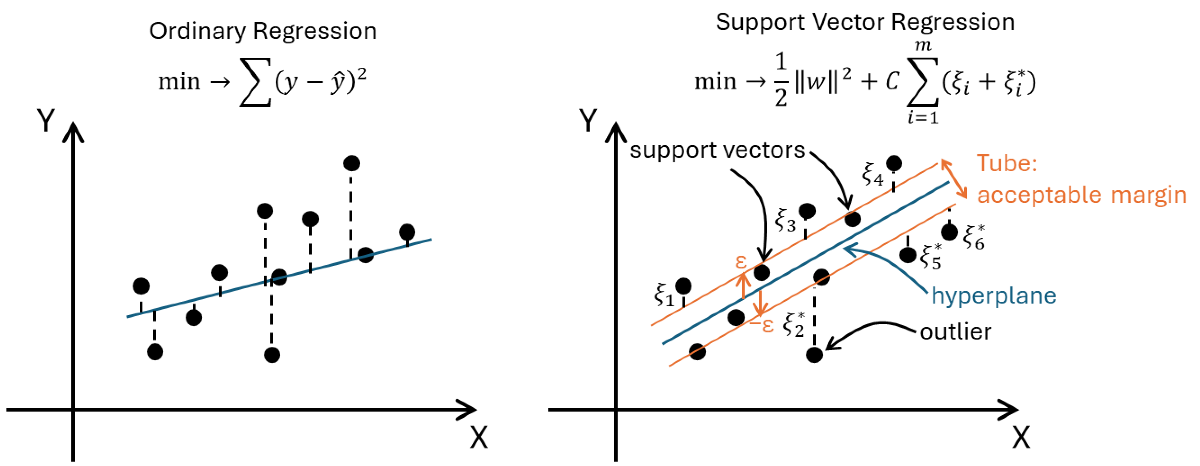
SVR is an extension of the SVM machine learning approach, used to solve regression problems [36,37]. In contrast to classification-oriented SVMs that aim to maximize class separation, SVR seeks to determine the hyperplane that minimizes the deviation from the data, within a defined error tolerance. The central idea of SVR is to find a hyperplane that is at a distance ε from all data points. Unlike ordinary regression that seeks to minimize the sum of squares of the residuals, SVR looks for a hyperplane that fits most of the data points within a specified and acceptable margin of error (see Figure 2). This distance ε defines a tube around the hyperplane, and the goal is to minimize the number of points that fall outside this tube. Support vectors are the data points that are at a distance ε from the regression hyperplane; that is, they are the points that are closest to the margin of error defined by the model. The equation that defines the hyperplane of a linear SVR would be:
y ^ = w , x + b ,
where y ^ is the hyperplane, w , x denotes the inner product between w and x , w is a vector of weights (coefficients), x is a vector of features (independent variables) and b is the constant term.
The goal of an SVR hyperplane is to find a balance between fitting the data and allowing for some errors, penalizing only those points that are outside the range ε. This approach makes the model more robust against outliers and improves its generalization ability, since a perfect fit of all data points is not required. Mathematically, the goal of the SVR can be written as follows, known as the primal problem:
min 1 2 w 2 + C i = 1 m ξ i + ξ i * , subject to restrictions: y i w T x i b ε + ξ i w T x i + b y i ε + ξ i * ξ i 0 ,   ξ i * 0
where C is a constant greater than or equal to zero that regulates the acceptable error, w 2 denotes the operation w T · w , ξ i ,   ξ i * is the error value (data outside the acceptable range ε) and m is the amount of data. For an SVR, C and ε are hyperparameters that a machine learning algorithm uses to control the learning process. These hyperparameters can be tuned from search combinations. Grid search is a systematical approach to find the optimal combination of hyperparameters that results in the best model performance.
To solve this optimization problem, dual formulation is introduced. This transformation has several advantages, such as the reduction in the number of variables and the possibility of using kernels to extend the model to nonlinear problems. The dual problem is obtained by forming the Lagrangian of a minimization problem using non-negative Lagrange multipliers ( α i and α i * ) to add the constraints to the objective function. A primary reason for formulating the dual problem in SVR and other convex optimization problems is to transform the original (primal) problem into a more computationally tractable form. Differentiating the Lagrangian function with respect to w provides a way to calculate the weights:
w = i = 1 m α i α i * x i
The primal problem involves variables such as w , b, ξ i and ξ i * , which can be difficult to handle directly. The dual problem eliminates w , ξ i and ξ i * , and works only with the Lagrange multipliers α i and α i * , which reduces complexity. The independent term b of the hyperplane equation is obtained from the condition of the so-called Karush–Kuhn-Tucker (KKT) technique. KKT conditions are a set of conditions necessary for a solution to be optimal in a constrained optimization problem [38]. In the context of SVR, these conditions help us to find the optimal values of the Lagrange multipliers ( α i and α i * ) that determine the decision hyperplane. The computational algorithm SMO (Sequential Minimal Optimization) of scikit-learn [39], a famous data analysis and machine learning tool, uses the KKT conditions as a guide to update the Lagrange multipliers. At each iteration, SMO selects two multipliers and updates them such that the KKT conditions are satisfied. This iterative process continues until a solution that satisfies all the KKT conditions is reached. To measure the error, a loss function known as the ε-insensitive loss is used, which only considers errors that are outside the ε margin. If the error is within this margin, it is considered zero. The loss is defined as [40]:
L ε = m a x ( 0 , y i y ^ ε ) ,
where y i is the real value and y ^ is the value predicted by the model or hyperplane.
The SMO algorithm functions as an iterative procedure that continues until all Lagrange multipliers satisfy the KKT conditions. These conditions are essential for validating the optimality of the solution, as they require that the partial derivative of the objective function with respect to each multiplier α be zero. This ensures that the solution corresponds to a stationary point, which may represent either a minimum or a maximum in the optimization landscape. The process of an SMO algorithm to train an SVR model is as follows [39]:
  • Initialization: The algorithm starts by initializing all the Lagrange multipliers { α 1 , α 1 * , α 2 , α 2 * , , α m , α m * } to zero.
  • Iterative Optimization:
    • Select the first pair of multipliers ( α i , α i * ): It searches for a pair of multipliers that violates the KKT conditions. This is the multiplier that is currently the “furthest” of its optimal value; for example, it has the largest prediction error.
    • Select the second pair of multipliers ( α j , α j * ): After finding the first, it then chooses a second multiplier that is likely to make the largest possible change to the first. This is done to speed up the convergence process.
    • Analytical Solution: Once the two pairs of multipliers, ( α i , α i * ) and ( α j , α j * ), are chosen, SMO solves a simple 2 × 2 sub-problem to find the optimal values for this pair. This sub-problem has a simple analytical solution, which avoids the need for complex, time-consuming numerical methods.
    • Updating Parameters and Repetition: After solving the sub-problem, the algorithm updates the values of ( α i , α i * ) and ( α j , α j * ). It then updates a parameter called the “bias” or b, which is essential for defining the regression function. The process from Step 2 is repeated until all α values converge and the KKT conditions are met for all data points.
  • End: Step 2 is repeated until all Lagrange multipliers satisfy the KKT conditions within a predefined tolerance. At this point, the algorithm converges, and the SVR optimization problem has been solved.
In this study, a seismic attenuation law for the classical intensity measure INp [11] is proposed using the SVR technique. The objective is to obtain the coefficients of a prediction model, whose general structure is detailed in Equation (1). In summary, the steps to develop GMPE from SVR are as follows:
  • Step 1: Obtain the weight vector ( w ) and Bias (b). The SMO algorithm, used by scikit-learn, solves the dual optimization problem to find the Lagrange multipliers ( α i and α i * ). Once these multipliers are found, they are used to compute the weight vector w and the bias b. The weight vector contains the coefficients for each independent variable in the GMPE. It is calculated with Equation (4).
  • Step 2: Formulate the Final GMPE. Once the weight vector w and the bias b have been calculated, the final GMPE can be expressed in a traditional linear form. The predicted value of INp is simply the dot product of the w vector and the input vector x , plus the bias term. The equation for the GMPE could be expressed as l o g ( I N p ) = w · x + b , where x is the input vector containing the values of your independent variables (e.g., magnitude, distance).
The process to obtain and prepare the data used to train the SVR model is described below.

3. The Generalized Bojorquez Intensity Measure IBg and the Particular Case INp

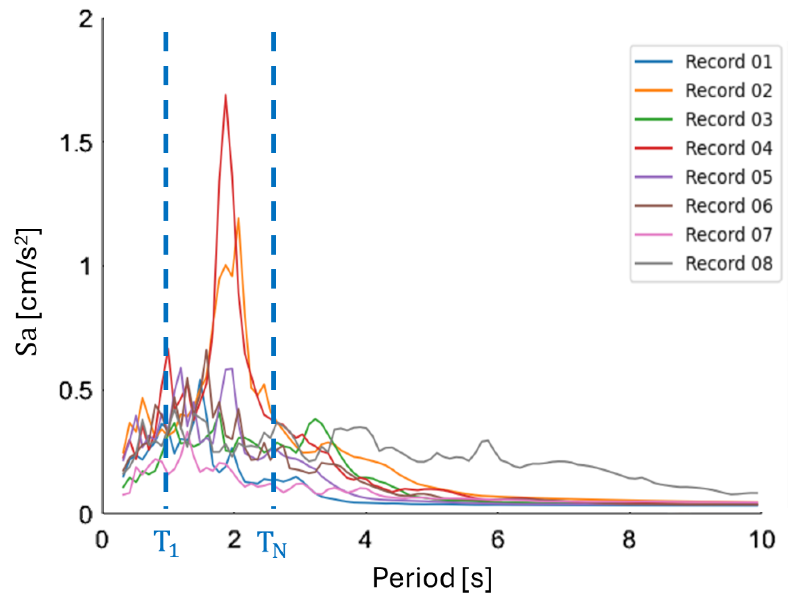
It has been discussed that IMs often try to capture the structural response through the spectral shape with varying degrees of success [41,42]. The most used intensity measure Sa(T1) is the perfect predictor for the response of SDOF elastic systems, and a good predictor for multi-degree-of-freedom (MDOF) elastic systems dominated by the first vibration mode, associated with structural period T1. However, Sa(T1) does not provide information about the spectral shape in other regions of the spectrum, which can be important for nonlinear behavior (beyond T1) or for structures dominated by higher modes (before T1) [5,6,10,11]. In the case of nonlinear vibration, the structure can be sensitive to different spectral values associated with a range of periods, for example, from the fundamental period T1 to a limiting value of interest called TN. To better illustrate some limitations of Sa(T1), let us consider a structure with a fundamental period T1 equal to 1.25 s subjected to a set of different seismic records. Figure 3 shows the response spectra of the set of records with significant site effects from Mexico City. For this example, the final period of interest is assumed to be TN equal to 2.5 s. The spectral ordinates are affected by a significant dispersion within <T1, TN>, which is likely to be reflected in the structural response. Therefore, intensity measures are required that provide information on the spectral shape over a complete region of the spectrum, such as a simple determination of the geometric mean, Saavg, between T1 and TN [15,30].
The geometric mean Saavg(T1, …, TN) is a particular case of a more complex expression known as the Generalized Bojorquez ground motion Intensity measure IBg [13]. The traditional form of IBg is defined as follows:
I B g = i = 1 i = N s S i T i α s i j = 1 j = N N p N p g α N p j k = 1 k = N f a f a α f a k ,
where it is observed that three fundamental parts constitute the expression. The first part is related to a spectral response, the second part is associated with the generalized spectral shape, while the third part is related to an auxiliary function. Even though the Saavg(T1, …, TN) could consider the spectral shape, this parameter only represents a particular spectral shape. The normalized geometric mean provides a method to connect the spectral shape with diverse spectral patterns. Here is where the generalized parameter Np (Npg) is introduced:
N p g = S a a v g T i , , T N S T j ,
S(Tj) represents a spectral parameter taken from any type of spectrum such as acceleration, velocity, displacement, input energy, inelastic parameters, etc., in the period Tj. Saavg(Ti,…,TN) is the geometric mean of a specific spectral parameter between the period range Ti and TN. Note that the periods Ti and Tj could be different. Npg is similar to the traditional definition of Np but for different types of spectra and a wider period range. Thus, the traditional parameter Np is a particular case of the generalized spectral shape parameter Npg. If the pseudoacceleration spectrum is used, and Ti = Tj = T1 (structural vibration period of the first mode), Npg is renamed to Np and it is expressed as follows:
N P = S a a v g T 1 , , T N S a T 1 ,
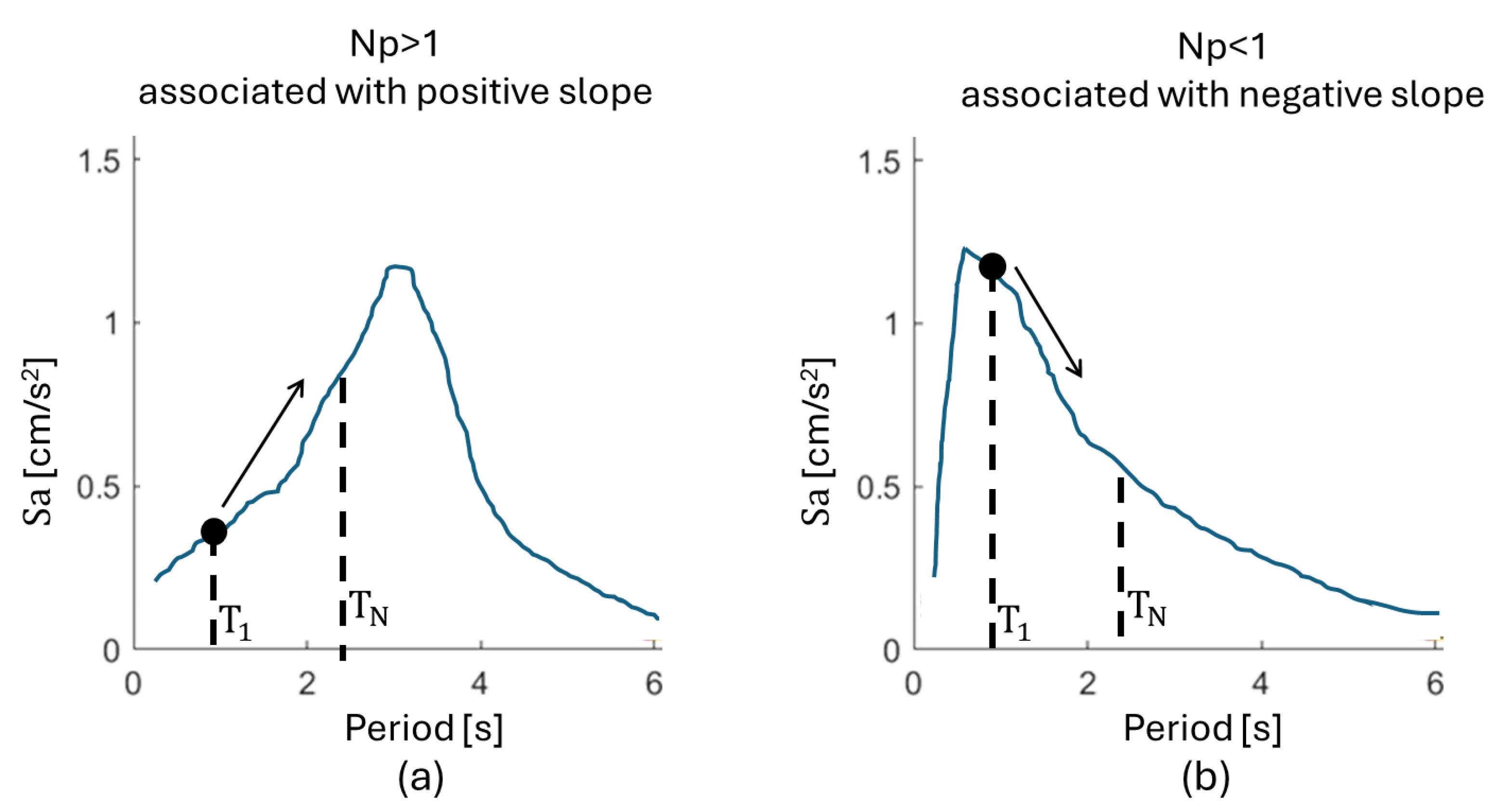
To consider a wide range of structural vibration periods after the first mode, in this study, TN = 2T1 is assumed. For example, the value of Np for the spectrum in Figure 4a in periods from T1 = 0.6 s to TN = 2T1 is 1.89; in the case of values of Np greater than 1, the spectra tend to increase beyond T1, while the spectra tend to decrease from T1 when Np is less than 1 (see Figure 4b).

The Particular Case INp

To account for nonlinear structural behavior in seismic response prediction, Bojórquez and Iervolino [11] proposed a scalar intensity measure based on spectral acceleration at the fundamental period. The specific definition of this intensity measure is a particular case of IBg where the first two parts of the expression are used in terms of Sa, and can be written as follows:
I N p = S a T 1 N p ,
where the parameter should be determined through regression analysis. Studies suggest optimal values ranging from 0 to 1, effectively weighting the contribution of higher-mode spectral accelerations relative to Sa(T1). Notably, Sa(T1) is a special case of INp when = 0 , while the average spectral acceleration, Saavg(T1, …, TN), corresponds to = 1 . Research developed by Bojórquez and Iervolino [11,16] indicates that values near 0.4 are optimal. Diverse studies have demonstrated the superior predictive capability of this intensity measure compared to other well-established measures [16,17,20]. This motivates the use of INp to propose a new ground motion prediction equation which will be very useful in computing seismic hazard analysis, seismic vulnerability, structural reliability, seismic resilience, etc.

4. Methodology

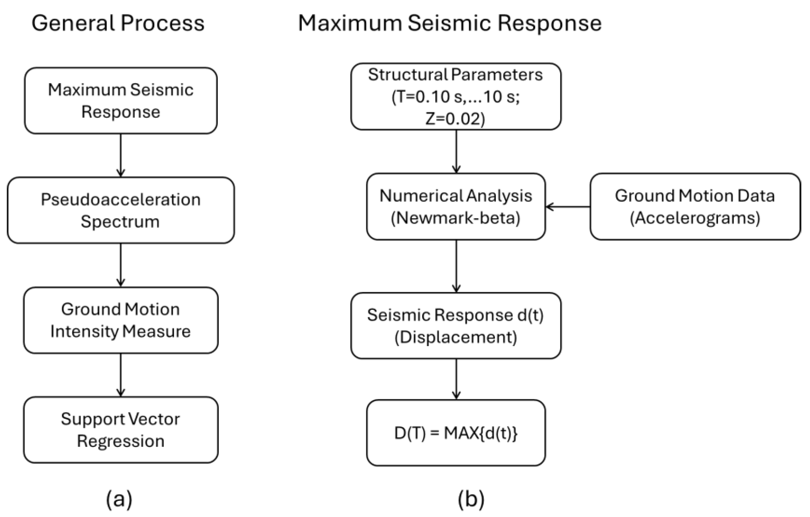
The main objective in order to propose ground motion prediction equations is to obtain the coefficients of Equation (1), where the variable of interest Y represents the ground motion intensity measure INp. The general process to obtain these coefficients is described in Figure 5a. This process is divided into 4 phases (maximum seismic response, pseudoacceleration spectrum and SVR), which are detailed below. To determine the maximum seismic responses in terms of displacement D (see Figure 5b), 990 structures were dynamically analyzed for periods T = 0.10, 0.11, 0.12, …, 10 s with damping Z = 5%; each one was subjected to 24 real seismic ground motions recorded (accelerograms) on firm ground in Mexico City. Using the Newmark-Beta Method, 23,760 time series were obtained to describe the seismic response d(t) of different structure–accelerogram combinations. According to Figure 6a, the pseudo-acceleration Sa(T1) is obtained from the multiplication of the natural frequency ω and the maximum displacement D. Meanwhile, Figure 6b shows the detailed procedure to estimate the IM INp using a loop, where the spectral shape Np of each structure with fundamental period T1 is considered.

Selected Seismic Ground Motion Records

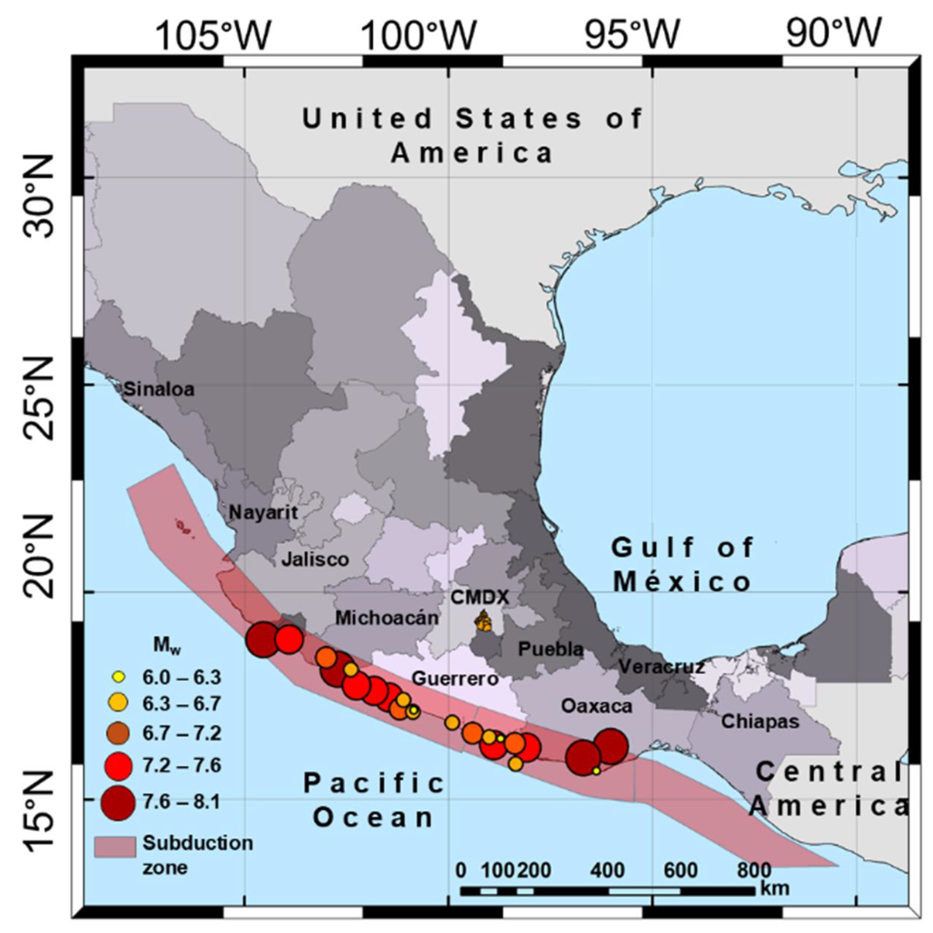
The Sa(T1) and INp spectra were obtained from 24 ground motions recorded at the firm-ground accelerometric station of Ciudad Universitaria (CU) in Mexico City. This firm-ground zone is integrated by volcanic bedrock and magma flows, with high shear-wave velocities (Vs30 ≈ 750 m/s) and short dominant soil periods [43,44], representing the target site conditions considered in the present study. In this context, the firm-ground CU station is selected as the reference site, given its extensive seismic record of major events affecting Mexico City since 1964 [45]. Additionally, most of ground motion prediction equations developed for Mexico City have been proposed from the seismic data recorded at this accelerometric station [7,33,46,47]. The location of the epicenters of these seismic events is shown in Figure 7. A close relationship between the epicenters and the Cocos plate subduction zone can be observed. Table 1 shows the magnitude Mw, distance R, depth H and date of the selected seismic records, which were obtained from the Strong Motion Network of the Institute of Engineering of the UNAM, Mexico (RAII-UNAM). All records were subjected to a linear baseline correction and were subjected to a band-pass filter. The minimum and maximum cut-off frequencies for the entire set of signals were 0.1 Hz and 25 Hz, respectively.
The ground motion records compiled correspond to interplate earthquakes, classified according to their focal mechanism. Interplate earthquakes are concentrated in the subduction zone where the Cocos and Rivera plates subduct beneath the North American plate, along the Mexican Pacific coast, more than 300 km from Mexico City [48]. These events are characterized by shallow thrust faults. All the selected accelerograms correspond to seismic events that represented a moderate to high level of hazard with Mw magnitudes equal to or greater than 6.

5. Numerical Results

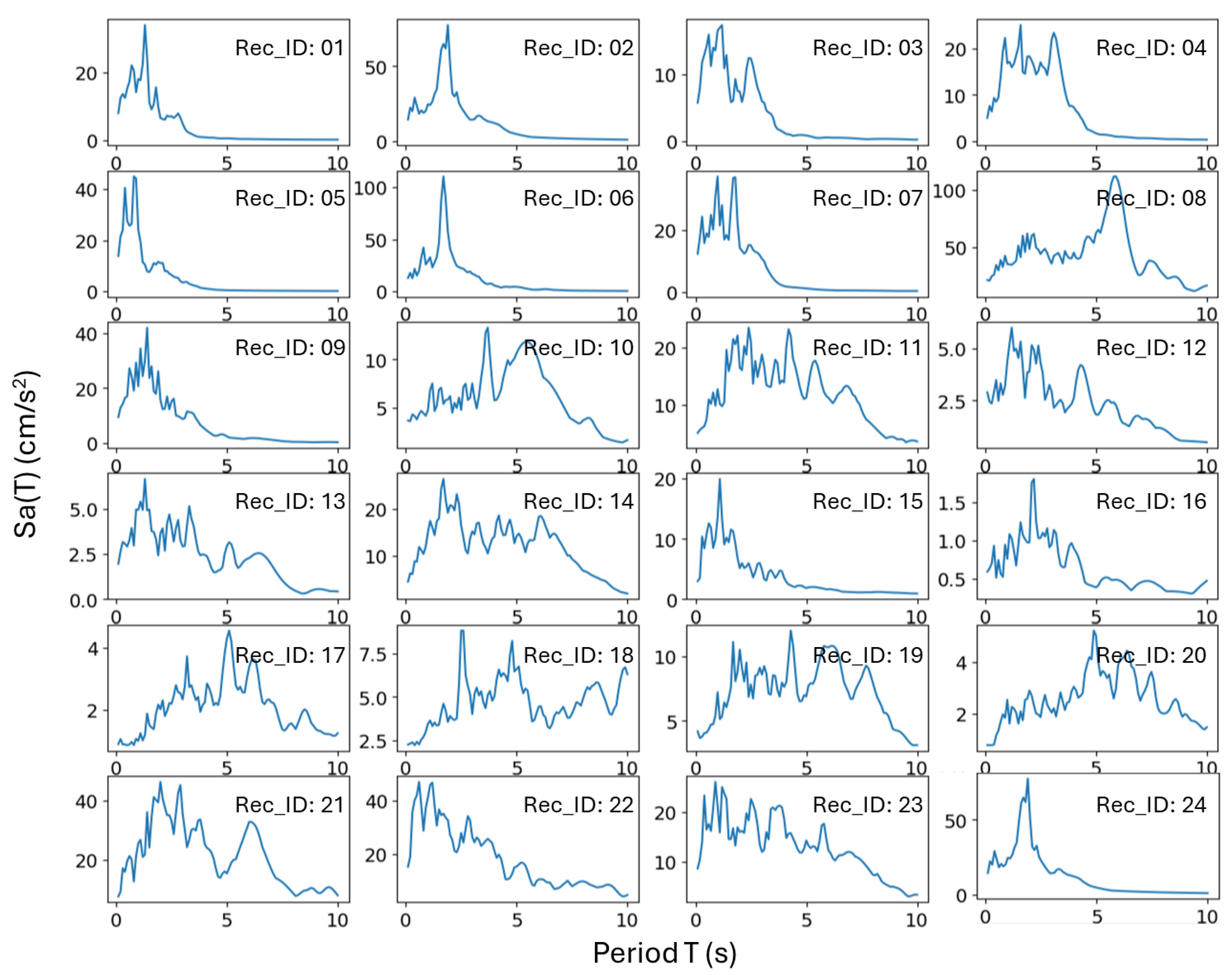
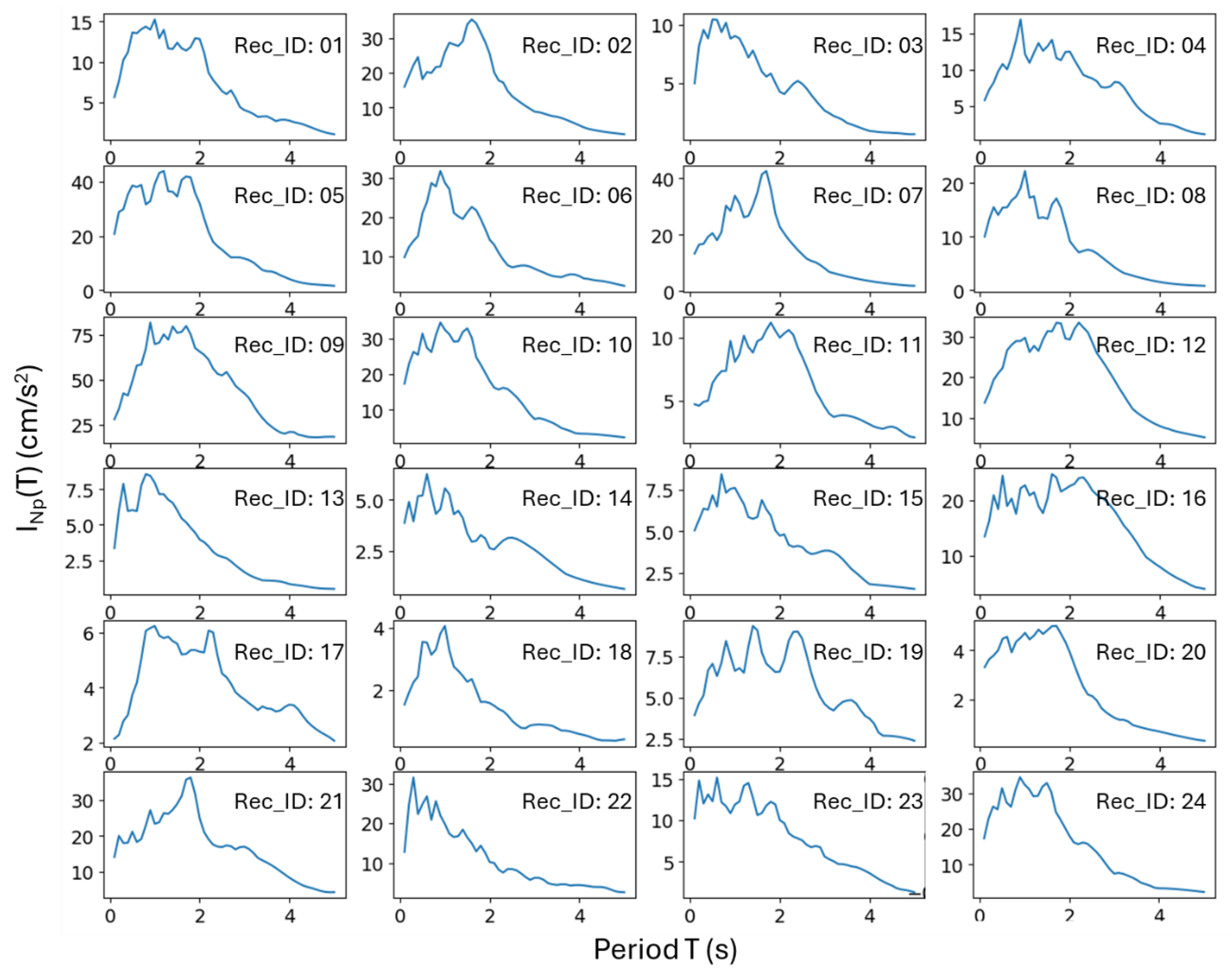
Figure 8 presents the 24 pseudo-acceleration spectra, where Sa(T) was estimated from the maximum responses of single-degree-of-freedom (SDOF) systems with structural periods ranging from T = 0 to 10 s. These spectra were derived using the procedure detailed in Figure 5a and show the considerable variability in the spectral shape across the selected ground motion records. This study proposes a ground motion prediction equation for the advanced intensity measure INp, which characterizes the destructive potential of earthquake ground motions given its capacity to capture the nonlinear response of structures. The intensity measure INp(T) was estimated for each ground motion record based on the spectral shape parameter Np, which was derived from its corresponding pseudo-acceleration spectrum. Accordingly, the values TN = 2T1 and α = 0.4 were adopted (Figure 9), following the recommendations of previous studies [11].
The INp data, calculated for various periods and each seismic event, is presented in Table 2. This structured format allows for the direct application of an SVR algorithm to analyze the information and derive the coefficient values for a prediction model.
Based on the variables in Table 2, the prediction model (or hyperplane) that best fits the data, considering a tolerance margin ε, is:
y ^ T = b T + w 1 T x 1 + w 2 T x 2 + w 3 T x 3 + w 4 T x 4 + σ T ,
where the independent term b and each coefficient w depend on a period T. The following expression rewrites the prediction model’s form into a notation more aligned with earthquake engineering:
l o g I N p T = c 1 T + c 2 T M w + c 3 T R + c 4 T l o g R + c 5 T H + σ T ,
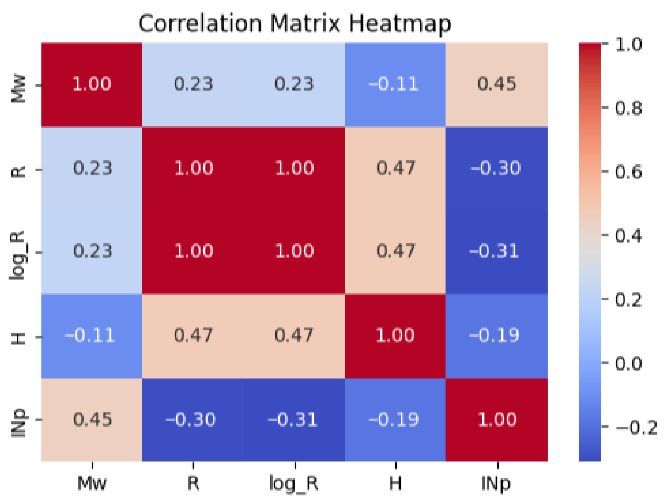
The correlation between these variables is illustrated in a heat map shown in Figure 10. A correlation matrix is a table that displays the correlation coefficients between different variables. Each cell in the matrix represents the correlation between a pair of variables. The correlation coefficient is the value in each cell (ranging from −1 to +1), which indicates the strength and direction of the relationship between two variables. Another way to represent the strength and direction of the relationship between variables is using a color scale. The multicollinearity check helps identify if any of the independent variables are highly correlated. In this case, deep red represents a correlation coefficient close to +1, while blue represents a correlation coefficient close to −0.30. The observed correlation between INp and the predictor variables suggests that these inputs can effectively contribute to the predictive capacity of the model.
SVR was employed to determine the coefficients c i of the prediction equation (Equation (1)), using data grouped according to structural period. A grid search procedure was performed to optimize the SVR hyperparameters C and ε, exploring values of C = [0.1, 1, 10, 100] and ε = [0.1, 1, 10, 100]. Grid search is a simple and widely used method for hyperparameter tuning in machine learning. Its purpose is to systematically find the optimal combination of hyperparameters that results in the best model performance. The resulting coefficients and their standard deviations for different periods are summarized in Table 3. The model exhibits a high coefficient of determination (R2) for periods shorter than 3 s, indicating good predictive performance. However, the R2 value is moderate for periods longer than 3 s.
Figure 11 compares the real INp spectra—computed through the deterministic procedure described previously—with those obtained from the GMPE defined by Equation (1), using the coefficients presented in Table 3. For a significant number of seismic events, the graphs reveal a strong similarity in shape between the observed (exact) spectra and those predicted by the regression-based equation.
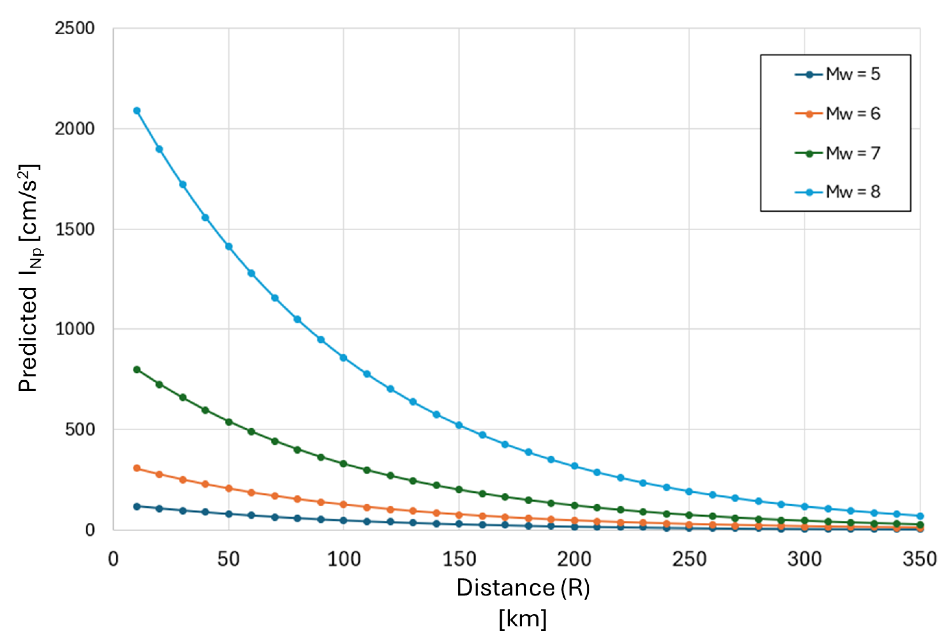
The attenuation behavior of INp is a crucial aspect of the prediction model, demonstrating a clear inverse relationship with increasing distance, as is expected for ground motion intensity. As shown in Figure 12, the predictive GMPE for a period T = 0.5 s accurately captures this expected behavior. The figure illustrates a consistent decrease in the predicted INp values as the source-to-site distance increases. Furthermore, it also correctly demonstrates the positive correlation between seismic magnitude and the predicted INp values. This behavior not only reinforces the physical validity of our SVR-based model but also confirms its ability to correctly reflect the fundamental principles of ground motion attenuation.
It is interesting to test the SVR algorithm to solve the regression problem encompassing all structural periods with only one expression or set of coefficients. For this purpose, the prediction equation would have the following form:
l o g I N p = c 1 + c 2 T + c 3 M w + c 4 R + c 5 l o g R + c 6 H + σ ,
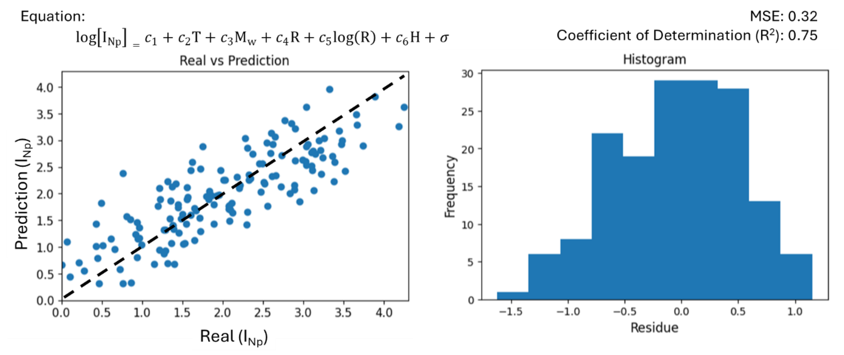
Figure 13 shows the result of applying the SVR algorithm with complete data to define a single expression that represents all the study periods. A good level of prediction is observed with an MSE of 0.32 and a coefficient of determination R2 of 0.75. Therefore, the prediction equation describes in general terms the ground motion intensity measure INp.
Applying ordinary linear regression, an error MSE = 0.37 and coefficient of determination R2 = 0.71 were obtained. These values suggest a solution with a slightly lower degree of prediction. However, SVR offers greater freedom of adjustment with the configuration of its hyperparameters.
To assess the model’s robustness, we performed a cross-validation study. The dataset was randomly split into a 70% training set and a 30% evaluation set. We repeated this process ten times, as shown in Table 4. The results in Table 4 show that the error variation is minimal. This suggests that the model’s performance is independent of the specific data split, confirming that dataset is enough to achieve a consistent and reliable prediction.

6. Model Limitations, Generalization and Application in Engineering Practice

Notice that although this is the first ground motion prediction equation proposed for INp in the literature, it is important to highlight that the dataset used in this study consists of 24 records from a single location, limited in scope. As a result, the model’s applicability is currently specific to the seismic and geotechnical conditions of the study area, which are characterized by interplate earthquakes recorded on firm rock sites. This work does not include data from different tectonic settings, nor does it account for records from soft soil sites, which are known to exhibit significant basin amplification and other complex effects. However, the primary objective of this study was to propose a foundational methodology for developing a ground motion prediction equation for the novel INp intensity measure, rather than to create a universally applicable model. The implementation and validation demonstrate the feasibility and effectiveness of using Support Vector Regression for this purpose. The rigorous cross-validation analysis, which showed consistent and robust results, further confirms the model’s stability and reliability within the studied data range.
Future research should focus on expanding this work by incorporating a much larger and more diverse dataset to include records from various tectonic settings and site conditions. This would be a crucial next step toward developing a more comprehensive and globally applicable GMPE for INp, especially in the development of future ground shaking maps, seismic and risk hazard maps, structural vulnerability and reliability assessment as well as to propose new seismic design approaches based on resilience concepts.

7. Conclusions

The first Ground Motion Prediction Equation for the INp intensity measure using a machine learning approach was developed. This represents a foundational step in seismic hazard analysis, as it provides a new tool that explicitly accounts for the influence of a ground motion’s spectral shape, an aspect often not considered by traditional intensity measures such as Sa(T1). The following conclusions have been drawn from the present study:
(1)
The Support Vector Regression (SVR) model demonstrated high predictive accuracy for periods shorter than 3 s. A grid search procedure was employed to optimize the hyperparameters C and ε (C = [0.1, 1, 10, 100] and ε = [0.1, 1, 10, 100]). The model’s performance was quantitatively confirmed with a coefficient of determination (R2) close to 0.80 and a Mean Squared Error (MSE) of 0.15, showing a strong correlation between the model’s predictions and the actual observed values.
(2)
The unified, generalized expression developed for the entire dataset proved to be a practical and valuable tool. It exhibited an acceptable coefficient of determination (R2) of 0.75 and a Mean Squared Error (MSE) of 0.32 for periods ranging from 0.1 to 5 s. This generalized equation provides a simple yet effective way for engineers and practitioners to estimate INp across a wide range of structural periods.
(3)
A comparison with ordinary linear regression (MSE = 0.37, R2 = 0.71) demonstrated the superior predictive performance of SVR. The versatility of SVR, through its adjustable hyperparameters C and ε, provides greater robustness, particularly against outliers.
(4)
To address concerns about the limited dataset, a rigorous cross-validation analysis was performed. The results showed a minimal variation in error across all data splits. This finding is crucial as it confirms that the model’s predictive accuracy is not dependent on a specific data split and that it possesses a strong capacity for generalization within the studied range.
(5)
This work not only introduces a novel GMPE but also validates the use of Support Vector Regression as a robust and effective method for developing these equations. Our findings offer a more sophisticated tool for seismic risk assessment, which can lead to more reliable estimations of seismic demand and, consequently, safer structural designs.

Author Contributions

Conceptualization, O.P.-S. and E.B.; methodology, J.B.; software, O.P.-S., E.B., J.B. and A.R.-C.; validation, S.E.R.; formal analysis E.B., O.P.-S. and J.B.; investigation, S.E.R.; resources, E.B.; data curation, R.C. and F.V.; writing—original draft preparation, O.P.-S. and E.B.; writing—review and editing, E.B., S.E.R., J.B. and A.R.-S.; visualization, O.P.-S. and A.R.-C.; supervision, E.B. and H.L.; project administration, E.B. and S.E.R.; funding acquisition, E.B. and S.E.R. All authors have read and agreed to the published version of the manuscript.

Funding

This research was developed thanks to economic support from the Secretaria de Ciencia, Humanidades, Tecnología e Innovación (SECIHTI), under Grant Ciencia de Frontera CF-2023-G-1636, and DGAPA-UNAM, under Grant PAPIIT-IN100423.

Institutional Review Board Statement

Not applicable.

Informed Consent Statement

Not applicable.

Data Availability Statement

The data used to support the findings of this study are available from the corresponding authors upon request.

Acknowledgments

We gratefully acknowledge the support of the Universidad Autónoma de Sinaloa for the PROFAPI project.

Conflicts of Interest

The authors declare no conflicts of interest.

Abbreviations

The following abbreviations are used in this manuscript:
GMPEGround Motion Prediction Equation
SVMSupport Vector Machine
SVRSupport Vector Regression
MSEMean Squared Error
IMIntensity Measures
PGAPeak Ground Acceleration
KKTKarush-Kuhn-Tucker
SMOSequential Minimal Optimization
SDOFSingle-Degree-of-Freedom
MDOFMulti-Degree-of-Freedom
UNAMUniversidad Nacional Autónoma de México
CUCiudad Universitaria

References

  1. Mehanny, S.S.; Cordova, P.P. Development of a Two-Parameter Seismic Intensity Measure and Probabilistic Design Procedure. J. Eng. Appl. Sci. 2004, 51, 233–252. [Google Scholar]
  2. Kazantzi, A.K.; Vamvatsikos, D. Intensity Measure Selection for Vulnerability Studies of Building Classes. Earthq. Eng. Struct. Dyn. 2015, 44, 2677–2694. [Google Scholar] [CrossRef]
  3. Supplement 3 for Minimum Design Loads and Associated Criteria for Buildings and Other Structures (ASCE/SEI 7-22). In Minimum Design Loads and Associated Criteria for Buildings and Other Structures; ASCE: Reston, VA, USA, 2021.
  4. Arzola, I.; Carlos, J.; Fortunio, C.; Energies, C. Manual de Diseño de Obras Civiles—Diseño Por Sismo CFE-IIE Versión; ResearchGate: London, UK, 2015; Volume 1. [Google Scholar]
  5. Asgarian, B.; Nojoumi, R.M.; Alanjari, P. Performance-Based Evaluation of Tall Buildings Using Advanced Intensity Measures (Case Study: 30-Story Steel Structure with Framed-Tube System). Struct. Des. Tall Spec. Build. 2014, 23, 81–93. [Google Scholar] [CrossRef]
  6. Baker, J.W.; Cornell, C.A. A Vector-Valued Ground Motion Intensity Measure Consisting of Spectral Acceleration and Epsilon. Earthq. Eng. Struct. Dyn. 2005, 34, 1193–1217. [Google Scholar] [CrossRef]
  7. Bojórquez, E.; Ruiz, S.E.; Rodríguez-Castellanos, A.; Orellana, M.A.; Reyes-Salazar, A.; Bojórquez, J. Bayesian Analysis-Based Ground Motion Prediction Equations for Earthquake Input Energy. Soil Dyn. Earthq. Eng. 2023, 173, 108115. [Google Scholar] [CrossRef]
  8. Grigoriu, M. Do Seismic Intensity Measures (IMs) Measure Up? Probabilistic Eng. Mech. 2016, 46, 80–93. [Google Scholar] [CrossRef]
  9. Kostinakis, K.; Fontara, I.K.; Athanatopoulou, A.M. Scalar Structure-Specific Ground Motion Intensity Measures for Assessing the Seismic Performance of Structures: A Review. J. Earthq. Eng. 2018, 22, 630–665. [Google Scholar] [CrossRef]
  10. Zaker Esteghamati, M.; Huang, Q. Evaluating the Impact of Higher-Mode and Inelastic Dynamic Responses of Concrete Frames on the Performance of Seismic Intensity Measures. Structures 2023, 56, 105029. [Google Scholar] [CrossRef]
  11. Bojórquez, E.; Iervolino, I. Spectral Shape Proxies and Nonlinear Structural Response. Soil Dyn. Earthq. Eng. 2011, 31, 996–1008. [Google Scholar] [CrossRef]
  12. Baker, J.W.; Cornell, C.A. Vector-Valued Intensity Measures Incorporating Spectral Shape for Prediction of Structural Response. J. Earthq. Eng. 2008, 12, 534–554. [Google Scholar] [CrossRef]
  13. Bojórquez, E.; Carvajal, J.; Ruiz, S.E.; Bojórquez, J. Reliability-Based Ductility Reduction Factors Surfaces Using the Generalized Bojorquez Ground Motion Intensity Measure IBg. Results Eng. 2024, 23, 102756. [Google Scholar] [CrossRef]
  14. Cordova, P.; Deierlein, G.; Mehanny, S.S.F.; Cornell, C.A. Development of A Two-Parameter Seismic Intensity Measure and Probabilistic Assessment Procedure. In Proceedings of the Second US-Japan Workshop on Performance-Based Earthquake Engineering Methodology for Reinforced Concrete Building Structures, Berkeley, CA, USA, 11–13 September 2000. [Google Scholar]
  15. Eads, L.; Miranda, E.; Lignos, D.G. Average Spectral Acceleration as an Intensity Measure for Collapse Risk Assessment. Earthq. Eng. Struct. Dyn. 2015, 44, 2057–2073. [Google Scholar] [CrossRef]
  16. Buratti, N. A Comparison of the Performances of Various Ground–Motion Intensity Measures. In Proceedings of the 15th World Conference on Earthquake Engineering, Lisbon, Portugal, 24–28 September 2012. [Google Scholar]
  17. Chen, Z.; Sun, X.; Feng, D.C.; Wu, G. Selection of Optimal Vector-Valued Seismic Intensity Measures for Fragility Analysis of Self-Centering Prestressed RC Structures. Bull. Earthq. Eng. 2024, 22, 1515–1538. [Google Scholar] [CrossRef]
  18. Javadi, E.; Yakhchalian, M. Selection of Optimal Intensity Measure for Seismic Assessment of Steel Buckling Restrained Braced Frames under Near-Fault Ground Motions. J. Rehabil. Civ. Eng. 2019, 7, 16. [Google Scholar] [CrossRef]
  19. Phan, H.N.; Paolacci, F.; Nguyen, V.M.; Hoang, P.H. Ground Motion Intensity Measures for Seismic Vulnerability Assessment of Steel Storage Tanks with Unanchored Support Conditions. J. Press. Vessel. Technol. Trans. ASME 2021, 143, 061904. [Google Scholar] [CrossRef]
  20. Rajabnejad, H.; Hamidi, H.; Naseri, S.A.; Abbaszadeh, M.A. Effect of Intensity Measure on the Response of a 3D-Structure under Different Ground Motion Duration. Int. J. Eng. Trans. B Appl. 2021, 34, 2219–2237. [Google Scholar] [CrossRef]
  21. Bojórquez, E.; Leyva, H.; Bojórquez, J.; Reyes-Salazar, A.; Mollaioli, F.; Barraza, M.; Torres, I. Optimal Acceleration and Energy-Based Record Selection Using Artificial Intelligence Approaches and NP. J. Earthq. Eng. 2023, 28, 582–601. [Google Scholar] [CrossRef]
  22. Modica, A.; Stafford, P.J. Vector Fragility Surfaces for Reinforced Concrete Frames in Europe. Bull. Earthq. Eng. 2014, 12, 1725–1753. [Google Scholar] [CrossRef]
  23. De Biasio, M.; Grange, S.; Dufour, F.; Allain, F.; Petre-Lazar, I. A Simple and Efficient Intensity Measure to Account for Nonlinear Structural Behavior. Earthq. Spectra 2014, 30, 1403–1426. [Google Scholar] [CrossRef]
  24. Tsioulou, A.; Galasso, C. Information Theory Measures for the Engineering Validation of Ground-Motion Simulations. Earthq. Eng. Struct. Dyn. 2018, 47, 1095–1104. [Google Scholar] [CrossRef]
  25. Kadas, K.; Yakut, A. Regression-Based Evaluation of Novel Intensity Measures under Alternative Ground Motion Record Sets. J. Phys. Conf. Ser. 2024, 2647, 252004. [Google Scholar] [CrossRef]
  26. Abrahamson, N.; Atkinson, G.; Boore, D.; Bozorgnia, Y.; Campbell, K.; Chiou, B.; Idriss, I.M.; Silva, W.; Youngs, R. Comparisons of the NGA Ground-Motion Relations. Earthq. Spectra 2008, 24, 45–66. [Google Scholar] [CrossRef]
  27. Arroyo, D.; García, D.; Ordaz, M.; Mora, M.A.; Singh, S.K. Strong Ground-Motion Relations for Mexican Interplate Earthquakes. J. Seismol. 2010, 14, 769–785. [Google Scholar] [CrossRef]
  28. Boore, D.M.; Joyner, W.B.; Fumal, T.E. Estimation of Response Spectra and Peak Accelerations from Western North American Earthquakes: An Interim Report; U.S. Geological Survey: Reston, VA, USA, 1993.
  29. Campbell, K.W.; Bozorgnia, Y. NGA-West2 Ground Motion Model for the Average Horizontal Components of PGA, PGV, and 5% Damped Linear Acceleration Response Spectra. Earthq. Spectra 2014, 30, 1087–1115. [Google Scholar] [CrossRef]
  30. Dávalos, H.; Miranda, E. A Ground Motion Prediction Model for Average Spectral Acceleration. J. Earthq. Eng. 2021, 25, 319–342. [Google Scholar] [CrossRef]
  31. Jaimes, M.A.; Ramirez-Gaytan, A.; Reinoso, E. Ground-Motion Prediction Model from Intermediate-Depth Intraslab Earthquakes at the Hill and Lake-Bed Zones of Mexico City. J. Earthq. Eng. 2015, 19, 1260–1278. [Google Scholar] [CrossRef]
  32. Molas, G.L.; Yamazaki, F. Attenuation of Earthquake Ground Motion in Japan Including Deep Focus Events. Bull.-Seismol. Soc. Am. 1995, 85, 1343–1358. [Google Scholar] [CrossRef]
  33. Ordaz, M.; Reyes, C. Earthquake Hazard in Mexico City: Observations versus Computations. Bull. Seismol. Soc. Am. 1999, 89, 1379–1383. [Google Scholar] [CrossRef]
  34. Chen, S.; Liu, X.; Fu, L.; Wang, S.; Zhang, B.; Li, X. Physics Symbolic Learner for Discovering Ground-Motion Models via NGA-West2 Database. Earthq. Eng. Struct. Dyn. 2024, 53, 138–151. [Google Scholar] [CrossRef]
  35. Barbur, V.A.; Montgomery, D.C.; Peck, E.A. Introduction to Linear Regression Analysis. Statistician 1994, 43, 339. [Google Scholar] [CrossRef]
  36. Guenther, N.; Schonlau, M. Support Vector Machines. Stata J. 2016, 16, 917–937. [Google Scholar] [CrossRef]
  37. Zhang, F.; O’Donnell, L.J. Support Vector Regression. In Machine Learning: Methods and Applications to Brain Disorders; Elsevier: Amsterdam, The Netherlands, 2019. [Google Scholar]
  38. Karush, W.; Kuhn, H.W.; Tucker, A.W.; Luptácik, M. Karush–Kuhn–Tucker Conditions. In Mathematical Optimization and Economic Analysis; Springer: Berlin/Heidelberg, Germany, 2008. [Google Scholar]
  39. Pedregosa, F.; Varoquaux, G.; Gramfort, A.; Michel, V.; Thirion, B.; Grisel, O.; Blondel, M.; Prettenhofer, P.; Weiss, R.; Dubourg, V.; et al. Scikit-Learn: Machine Learning in Python. J. Mach. Learn. Res. 2011, 12, 2825–2830. [Google Scholar]
  40. Platt, J.C.; Labs, R. Sequential Minimal Optimization: A Fast Algorithm for Training Support Vector Machines Review. In Advances in Kernel MethodsSupport Vector Learning; MIT Press: Cambridge, MA, USA, 1997; Volume 208. [Google Scholar]
  41. Giovenale, P.; Cornell, C.A.; Esteva, L. Comparing the Adequacy of Alternative Ground Motion Intensity Measures for the Estimation of Structural Responses. Earthq. Eng. Struct. Dyn. 2004, 33, 951–979. [Google Scholar] [CrossRef]
  42. Huang, C.; Galasso, C. Ground-Motion Intensity Measure Correlations Observed in Italian Strong-Motion Records. Earthq. Eng. Struct. Dyn. 2019, 48, 1634–1660. [Google Scholar] [CrossRef]
  43. Auvinet, G.; Juárez, M. Geotechnical Characterization of Mexico City Subsoil. In Proceedings of the 2011 Pan-Am CGS Geotechnical Conference, Toronto, ON, Canada, 2 October 2011. [Google Scholar]
  44. Singh, S.K.; Cruz-Atienza, V.; Pérez-Campos, X.; Iglesias, A.; Hjörleifsdóttir, V.; Reinoso, E.; Ordaz, M.; Arroyo, D. Deadly Intraslab Mexico Earthquake of 19 September 2017 (Mw 7.1): Ground Motion and Damage Pattern in Mexico City. Seismol. Res. Lett. 2018, 89, 2193–2203. [Google Scholar] [CrossRef]
  45. Singh, S.K.; Ordaz, M.; Pérez-Campos, X.; Iglesias, A. Intraslab versus Interplate Earthquakes as Recorded in Mexico City: Implications for Seismic Hazard. Earthq. Spectra 2015, 31, 795–812. [Google Scholar] [CrossRef]
  46. Jaimes, M.A.; Reinoso, E.; Ordaz, M. Comparison of Methods to Predict Response Spectra at Instrumented Sites given the Magnitude and Distance of an Earthquake. J. Earthq. Eng. 2006, 10, 887–902. [Google Scholar] [CrossRef]
  47. Ordaz, M.; Singh, S.K.; Arciniega, A. Bayesian Attenuation Regressions: An Application to Mexico City. Geophys. J. Int. 1994, 117, 335–344. [Google Scholar] [CrossRef]
  48. Lermo, J.; Santoyo, M.A.; Jaimes, M.A.; Antayhua, Y.; Chavacán, M. Local Earthquakes of the Mexico Basin in Mexico City: κ, Q, Source Spectra, and Stress Drop. Bull. Seismol. Soc. Am. 2016, 106, 1423–1437. [Google Scholar] [CrossRef]
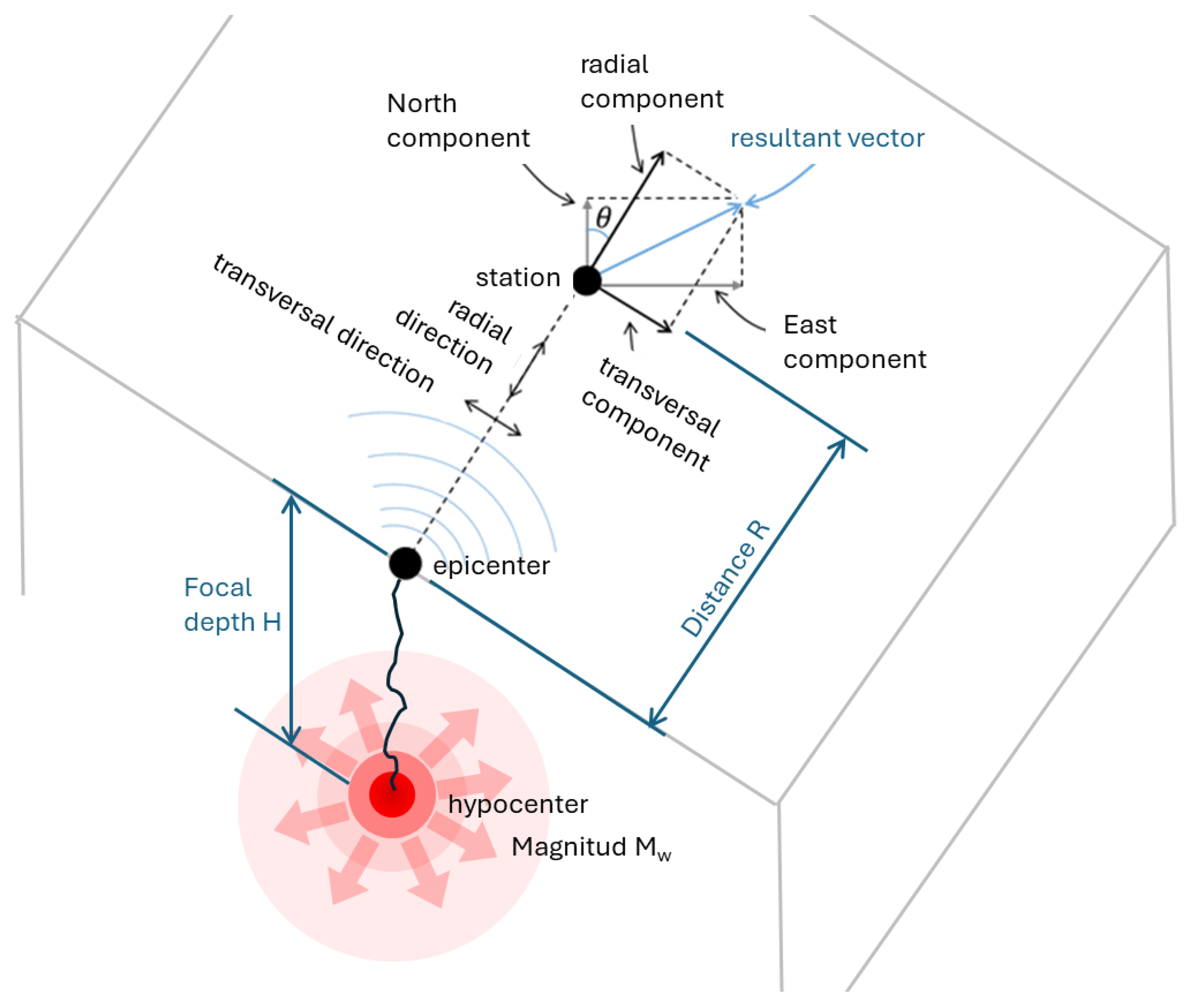
Figure 1. Fundamental parameters influencing ground motion at a seismic station.
Ai 06 00254 g001
Figure 2. Ordinary regression and Support Vector Regression.
Ai 06 00254 g002
Figure 3. Sa(T1) response spectra for ground motions recorded on soft soil sites of Mexico City.
Ai 06 00254 g003
Figure 4. Np behavior according to the spectral shape. (a) positive slope and (b) negative slope.
Ai 06 00254 g004
Figure 5. Flowcharts. (a) General process. (b) Maximum structural response.
Ai 06 00254 g005
Figure 6. Flowcharts for the computation of response spectra considering: (a) pseudo-acceleration Sa(T1) and (b) the intensity measure INp.
Ai 06 00254 g006
Figure 7. Epicentral locations of the earthquake events used in this study (see Table 1).
Ai 06 00254 g007
Figure 8. Sa(T) spectra response corresponding to the ground motion records selected.
Ai 06 00254 g008
Figure 9. INp(T) spectra response derived from the Sa(T) spectra shown in the previous figure.
Ai 06 00254 g009
Figure 10. Correlation matrix between ground motion parameters and INp.
Ai 06 00254 g010
Figure 11. Comparison between the observed INp response spectra and those predicted using the proposed GMPE.
Ai 06 00254 g011
Figure 12. Prediction of the INp in terms of magnitude and distance for a structural period of 0.5 s.
Ai 06 00254 g012
Figure 13. SVR results using complete data to derive a unified GMPE for INp.
Ai 06 00254 g013
Table 1. Seismic events recorded by the CU Station in the RAII-UNAM dataset online.
IDDate M w R
(km)
H
(km)
IDDate M w R
(km)
H
(km)
123 August 19657.8466161331 May 19906.130421
22 August 19687.4326331415 May 19936.032020
319 March 19786.4285161524 October 19936.731019
429 November 19787.8414191614 September 19957.332022
514 March 19797.628720179 October 19958.053027
625 October 19817.3330201815 July 19966.630120
77 June 19826.9304151919 July19976.739415
87 June 19827.030315203 February 19986.350933
919 September 19858.129515219 August 20006.538033
1021 September 19857.6318152220 March 20127.432916
1130 April 19867.0409162318 April 20147.230410
1225 April 19896.929019248 May 20146.439817
Table 2. Data organization and relationship with prediction equations.
IndexPeriod
T
(s)
Magnitude Distance l o g R x 3 Depth INp
(cm/s2)
l o g I N p y
M w x 1 R x 2
(km)
H x 4
(km)
00.17.84666.144186165.6130241.72509
10.117.84666.144186165.8887861.77305
20.127.84666.144186166.2366131.830437
........................
11,2904.986.42985.697093171.4060410.340778
11,2914.996.42985.697093171.3892470.328762
11,29256.42985.697093171.3305350.285581
Table 3. Coefficients of the prediction equation.
TMSER2Intercept
c 1
Coef Mw
c 2
Coef R
c 3
Coef log(R)
c 4
Coef H
c 5
Std Dev
0.10.080.85−0.500.86−0.010.010.010.29
0.20.110.82−0.240.91−0.010.040.000.33
0.30.120.82−0.160.91−0.01−0.010.010.33
0.50.130.77−0.590.96−0.010.010.000.35
1.00.110.81−1.491.02−0.010.010.010.32
2.00.180.77−2.861.02−0.010.090.030.42
3.00.220.72−3.740.95−0.010.090.010.47
4.00.290.61−4.540.940.000.070.000.54
5.00.390.52−5.050.920.000.050.000.62
Table 4. Cross-validation study.
IDMSE Training DataMSE Evaluation Data
10.34500.3520
20.31450.3235
30.33200.3420
40.32140.3315
50.33510.3452
60.31700.3260
70.34430.3533
80.32460.3335
90.33300.3410
100.33020.3413
Disclaimer/Publisher’s Note: The statements, opinions and data contained in all publications are solely those of the individual author(s) and contributor(s) and not of MDPI and/or the editor(s). MDPI and/or the editor(s) disclaim responsibility for any injury to people or property resulting from any ideas, methods, instructions or products referred to in the content.