A Step Towards Neuroplasticity: Capsule Networks with Self-Building Skip Connections

Abstract

Background: Integrating nonlinear behavior into the architecture of artificial neural networks is regarded as essential requirement to constitute their effectual learning capacity for solving complex tasks. This claim seems to be true for moderate-sized networks, i.e., with a lower double-digit number of layers. However, going deeper with neural networks regularly turns into destructive tendencies of gradual performance degeneration during training. To circumvent this degradation problem, the prominent neural architectures Residual Network and Highway Network establish skip connections with additive identity mappings between layers. Methods: In this work, we unify the mechanics of both architectures into Capsule Networks (CapsNet)s by showing their inherent ability to learn skip connections. As a necessary precondition, we introduce the concept of Adaptive Nonlinearity Gates (ANG)s which dynamically steer and limit the usage of nonlinear processing. We propose practical methods for the realization of ANGs including biased batch normalization, the Doubly-Parametric ReLU (D-PReLU) activation function, and Gated Routing (GR) dedicated to extremely deep CapsNets. Results: Our comprehensive empirical study using MNIST substantiates the effectiveness of our developed methods and delivers valuable insights for the training of very deep nets of any kind. The final experiments on Fashion-MNIST and SVHN demonstrate the potential of pure capsule-driven networks with GR.

1. Introduction

The depth of neural architectures is known as a crucial factor for the ease of learning complex tasks by enriching the representational capacity of neural systems with further abstraction levels. Hence, the exceptional role of depth is particularly manifested in the term deep learning itself. Despite the great potential of going deeper with neural networks, one encounters various difficulties in practice that negatively influence or even completely stall network optimization during the course of training. A de facto standard strategy against such a difficulty constitutes Batch Normalization (BN) [1] that normalizes feature distributions in order to prevent the problem of exponentially growing or decreasing gradients caused by an enlarged amount of stacked layers. Although there is perceived numerical stability in the optimization process of deeper neural networks, the resulting model performance gradually degenerates with an increase in network depth, which is commonly referred to as the degradation problem [2,3,4,5,6,7].

Figure 1 and

Table 1. Final training accuracies (in %) for distinct activation functions using a network depth of 90 intermediate blocks.

Configuration		Best	AVG
Plain Net	linear	$47.52$	$41.92\pm \phantom{0}9.21$
	ReLU	$33.77$	$20.15\pm \phantom{0}7.13$
	Leaky ReLU	$44.94$	$31.70\pm 11.75$
	ELU	$77.38$	$56.98\pm 14.09$
	tanh	$19.65$	$18.43\pm \phantom{0}1.09$
	sigmoid	85.21	$\underline{\mathbf{68}.\mathbf{00}}\pm 20.80$
CapsNet	SR+linear	$43.67$	$41.68\pm \phantom{0}2.43$
	SR+sigmoid	$72.93$	$\underline{\mathbf{68}.\mathbf{75}}\pm \phantom{0}3.98$
	SR+Leaky ReLU	$63.17$	$37.90\pm 13.99$
	SR+squash	$\underline{\mathbf{89}.\mathbf{48}}$	$57.66\pm 30.92$
	k-MR+squash	$11.23$	$11.23\pm \phantom{0}0.00$
	DR+squash	$11.23$	$11.23\pm \phantom{0}0.00$

serve as the first empirical evidence concerning the degradation problem regarding conventional neural networks and Capsule Networks (CapsNet)s [8,9], based on the simple MNIST [10,11] classification dataset of handwritten digits. Specifically, CapsNets organize their network layers in capsules [12] consisting of equal-sized neuron groups and conduct a predefined routing procedure to steer signal propagation from lower-layer capsules to higher-layer ones [8,9]. CapsNets were previously applied on various application tasks such as image recognition [8,9], text classification [13,14,15], visual smoke and fire detection [16], or in medical research [17]. Performance degradation occurs with a gain in network depth independent from the neural architecture across a variety of activation functions (i.e., Rectified Linear Unit (ReLU) [18,19], Leaky ReLU [20], Exponential Linear Unit (ELU) [21], the tangens hyperbolicus and the logistic sigmoid). To isolate potential overfitting effects from our consideration of the degradation problem, we provide at this point model accuracy solely based on the training set. We will address the generalization ability of a pure capsule-driven architecture in the final experiment. However, the concrete activation function appears as a critical hyperparameter for governing the intensity of degenerative effects. The same observation holds for the selected routing procedure in CapsNets (including Static Routing (SR) [13], k-Means Routing (k-MR) [14], Dynamic Routing (DR) [8] and the squash [8] nonlinearity). In accordance with previous work [22,23], the degradation problem also arises for the linear case where the activation function equals the identity function.

An intuition of this circumstance can be conveyed with the recursive expression of a network block with linear activation using BN:

$$\begin{array}{c}{\overline{\mathbf{h}}}_i(\mathbf{x};l):=\mathrm{BN}\left(\sum _j{w}_{ij}^{\left(l\right)}{\overline{\mathbf{h}}}_j(\mathbf{x};l-1)\right),\hfill \\ {\overline{\mathbf{h}}}_i(\mathbf{x};1):=\mathrm{BN}\left({\mathbf{w}}_1^T\mathbf{x}\right).\hfill \end{array}$$

(1)

Since BN applies a static nonlinear transformation per batch, the neural activity ${\overline{\mathbf{h}}}_i(\mathbf{x};l)$ of the i-th neuron in the l-layer for an input sample $\mathbf{x}\in {\mathbb{R}}^d$ can be straightforwardly interpreted as the iterative weighted mean over all previous layers. Assuming a random weight vector initialization, the linear neural network degenerates to a single path of repeated linear mixtures with nonlinear distortions induced by BN. We denominate the destructive tendency to dilute highly informative neuron outputs through iterative summation over all available signals as information diffusion. We further ascribe information diffusion to the inability of a neural network to select a subset of relevant input signals per neuron.This problem formulation explicitly includes nonlinear effects (e.g., from BN and activation functions), as opposed to theoretical analyses [22,23]. Figure 1 demonstrates that specific activation functions can mitigate or amplify information diffusion up to a certain extent of network depth.

The most promising technique to effectively overcome the degradation problem includes the implementation of skip connections that bypass outputs from previous layers as additive components to the input of deeper layers in the network hierarchy. The idea of skip connections essentially constitutes two distinct types of network architectures, namely Residual Networks [5,6] and Highway Networks [3,4]. In residual networks, skip connections are realized as static shortcuts between predefined blocks comprising several stacked network layers [5,6], whereas highway networks dynamically create skip connections via parametric neural gates between regular network layers [3,4]. The rationale behind both types is the facilitation of identity mappings which limit the effective depth of a neural network to the needed representational capacity demanded by a specific application task. At the level of network layers, skip connections especially constitute implicit paths of neural information processing that exponentially increase with a gain in network depth and behave like a network ensemble [24]. It is observed that the presence of skip connections at the time of training attenuates degradation effects on the performance of single-path feed-forward networks during inference [7]. A current explanation for this beneficial behavior is the solving of the near-singularity problem, where skip connections prevent neural computations from collapsing into singular feature spaces [22,23]. Hence, it is not surprising that other techniques even mimic the functionality of skip connections using specific initialization strategies [25] or learnable scaling parameters in combination with kernel updates [26].

Interestingly, the inherent structure of CapsNets in combination with a suitable routing procedure provides the potential to learn parametric skip connections during network optimization. Encouraging CapsNets to establish self-building skip connections leads to one implicit path of neural information processing for each capsule in a layer, while classical residual and highway networks are limited to a single implicit path per layer. This is in line with the next evolutionary stage of residual networks, namely ResNeXt [27], which aggregates residual transformations over multiple paths within predefined blocks and proved superior performance against its single-path predecessor. Again, CapsNets embody the more generic variant to ResNeXt without the need for explicit block design or static bottleneck structures between residual parts. As a natural consequence, CapsNets with self-building skip connections take a step towards structural neuroplasticity after the desired credo one architecture fits it all. The central contribution of our paper is three-fold:

• Firstly, we theoretically unify the skip connection mechanisms of residual networks and highway networks into CapsNets by showing their functional equivalence under certain conditions. Moreover, we identify the necessary preconditions to facilitate the shaping of self-building skip connections within CapsNets. Our theoretical findings provide direct implications for the design of arbitrary neural architectures by demystifying specific properties of their dynamics.
• Secondly, we introduce the concept of Adaptive Nonlinearity Gates by means of practical methods that fulfill the necessary preconditions and help to stabilize the training of very deep networks in general. These methods comprise straightforward strategies like biased BN, parametric activation functions and adaptive signal propagation. In particular, we present the novel Doubly-Parametric ReLU activation function and design the Gated Routing procedure dedicated to the training of enormously deep CapsNets.
• Thirdly, we supply a comprehensive experimental study to substantiate our theoretical findings and the proposed methods. The empirical results reveal valuable insights for the optimization of very deep neural networks of any kind. Specifically, our strategies prove to effectively mitigate the degradation problem.

The paper is structured according to our contributions: Section 2 starts with a theoretical derivation of an equivalence relationship between the computations in residual networks, highway networks and CapsNets. Section 3 comprises the definition of practical methods to bring very deep neural networks in a desirable condition to promote stable optimization, and presents a novel routing algorithm between layers in a CapsNet to resist the degradation problem. In Section 4, we systematically conduct experiments to validate our theoretical insights and empirically prove the effectiveness of our devised approaches. The study design is driven by the formulation and subsequent answering of dedicated research questions. Section 5 draws the important implications of our work in the context of related topics. Section 6 concludes with the major findings of the paper.

2. Theory

2.1. Skip Connection Pattern

In Residual Learning [5,6], a network layer is formulated as a residual unit that conducts the mapping

$${\mathcal{H}}_{\mathcal{G}}^{\left(R\right)}\left(\mathbf{x}\right)=\varphi \left(\mathcal{F}\left(\mathbf{x}\right)+\mathcal{G}\left(\mathbf{x}\right)\right)$$

(2)

where $\mathcal{F}\left(\mathbf{x}\right)$ means a residual function as output from a single or stacked conventional layers, $\mathbf{x}$ denotes the input signal to the residual unit, and $\varphi$ equals the activation function. The mapping $\mathcal{G}\left(\mathbf{x}\right)$ usually corresponds to the identity function to support stable gradient flow over arbitrary paths of neural information processing [6]. Introducing a projection matrix W is a valid strategy to ensure the same dimensionality in the summation for the general case [5], which specifies Equation (2) as

$${\mathcal{H}}^{\left(R\right)}\left(\mathbf{x}\right)=\varphi \left(\mathcal{F}\left(\mathbf{x}\right)+W\mathbf{x}\right).$$

(3)

The computational graph for Equation (3) is visualized in subfigure (a) of Figure 2.

Subfigure (b) transfers the residual mechanism from (a) to CapsNets by presenting an atomic pattern for a self-building skip connection between consecutive capsule layers. We prefer the term skip connection [4,6] against shortcut connection [5] since the CapsNet rather passes signals silently than abbreviating processing paths. In the CapsNet snippet three fully-connected layers with $\{1,2,1\}$ capsules are shown. Specifically, we declare the left path as a residual function $\mathcal{F}\left(\mathbf{x}\right)$ and the right path, emphasized in red, as a skip connection. For simplicity, bias weights are completely omitted. The exemplary CapsNet utilizes Static Routing (SR) [13] as inter-layer dynamics, leading to the computation rule for a capsule ${\mathbf{c}}_i$ in the $(l+1)$-layer of

$${\mathbf{c}}_i^{(l+1)}=\varphi \left(\sum _j{W}_{ij}^{(l+1)}{\mathbf{c}}_j^{\left(l\right)}\right)$$

(4)

where $\varphi$ denotes the used nonlinearity and $W_{ij}^{(l+1)}$ represents an individual transformation matrix between a higher-layer capsule and a lower-layer one. As its name indicates, SR simply propagates all signals from a previous layer to each capsule in the subsequent layer. Contrary to the classic description of SR [13], we generalize the nonlinearity $\varphi$ instead of applying the squash [8] function. In the progress of this section, we will explain this design decision. First, we want to harmonize Equation (4) with Equation (3). Denominating the first capsule in subfigure (b) of Figure 2 as input vector $\mathbf{x}$ and the final capsule as mapping $\mathcal{H}\left(\mathbf{x}\right)$ we obtain the computation rule

$$\begin{array}{cc}\hfill {\mathcal{H}}^{\left(C\right)}\left(\mathbf{x}\right)& =\varphi \left[W_{\mathcal{F}}^{\left(l\right)}\varphi \left(W_{\mathcal{F}}^{(l-1)}\mathbf{x}\right)+W_{\mathcal{S}}^{\left(l\right)}\varphi \left(W_{\mathcal{S}}^{(l-1)}\mathbf{x}\right)\right]\hfill \\ \hfill & =\varphi \left[\mathcal{F}\left(\mathbf{x}\right)+W_{\mathcal{S}}^{\left(l\right)}\varphi \left(W_{\mathcal{S}}^{(l-1)}\mathbf{x}\right)\right]\hfill \end{array}$$

(5)

where the subscript $\mathcal{F}$ and $\mathcal{S}$ of the weight matrices signals belonging to the residual function or the skip connection, respectively. The superscript $\left(C\right)$ specifies $\mathcal{H}\left(\mathbf{x}\right)$ in the context of CapsNets. If we now assume the following conditions hold:

$$\begin{array}{cc}\hfill & \left(1\right)\forall x\in [I_1,I_2]:\varphi \left(x\right)\cong \lambda x,\hfill \\ \hfill & \left(2\right){\left(W_{\mathcal{S}}^{(l-1)}\mathbf{x}\right)}_i\in [I_1,I_2],\hfill \end{array}$$

(6)

meaning that the activation function $\varphi$ contains a suitable interval $[I_1,I_2]$ with exact or approximative linear progress, and the first transformation matrix $W_{\mathcal{S}}^{(l-1)}$ of the skip connection projects the components of $\mathbf{x}$ onto the interval $[I_1,I_2]$. From these assumptions, we can deduce an equivalence relationship between Equations (5) and (3) by

$$\begin{array}{cc}\hfill \Rightarrow {\mathcal{H}}^{\left(C\right)}\left(\mathbf{x}\right)& =\varphi \left(\mathcal{F}\left(\mathbf{x}\right)+\lambda ·W_{\mathcal{S}}^{\left(l\right)}{W}_{\mathcal{S}}^{(l-1)}\mathbf{x}\right)\hfill \\ \hfill & =\varphi \left(\mathcal{F}\left(\mathbf{x}\right)+W_{{\mathcal{S}}^{\prime }}\mathbf{x}\right)\hfill \\ \hfill & \equiv {\mathcal{H}}^{\left(R\right)}\left(\mathbf{x}\right)\hfill \end{array}$$

(7)

where $W_{{\mathcal{S}}^{\prime }}$ subsumes both weight matrices from the skip connection and the scaling factor $\lambda \in \mathbb{R}\setminus \left\{0\right\}$. This leads to an equivalent version of a regular shortcut connection with the projection matrix, as displayed in Equation (3). It is now clear why the nonlinearity $\varphi$ in the CapsNet needs to be abstracted to an activation function that satisfies the conditions in Equation (6).

It is noteworthy that the use of a projection matrix weakens the intention behind residual learning to facilitate identity mappings. Moreover, the experiments in [6] suggest a clear advance of exact identity mappings against linear approximations. Nevertheless, we will resolve this apparent contradiction by systematically identifying the necessary preconditions to avert obstacles in approaching identity mappings within CapsNets during network optimization. Note that in the primary paper [5] about residual learning the additional parameter investment in projection matrices improved model performance for moderate-sized residual networks (≈30 units), while successive work [6] reported degenerative effects when linearly manipulating skip connection signals in enlarged networks (≈100 units). This situation indicates conceptual flaws in conventional network design which amplify with an increase in depth.

2.2. Multi-Layered Skip Paths

Highway Networks [3,4] integrate parametric neural gates in their architecture to establish direct information flow across multiple consecutive layers. Contrary to residual learning, highway networks, implicitly rather than explicitly, steer information flows in the direction of the vertical depth in a neural network [3,4]:

$${\mathcal{H}}^{\left(H\right)}\left(\mathbf{x}\right)=\mathcal{F}\left(\mathbf{x}\right)\odot \mathcal{T}\left(\mathbf{x}\right)+\mathbf{x}\odot \mathcal{C}\left(\mathbf{x}\right)$$

(8)

where the vector $\mathbf{x}$ means the input to a highway layer and the operator ⊙ denotes the element-wise product. $\mathcal{F}\left(\mathbf{x}\right)$, $\mathcal{T}\left(\mathbf{x}\right)$ and $\mathcal{C}\left(\mathbf{x}\right)$ are arbitrarily parameterized nonlinear mappings, e.g., defined as regular network layers, with the same output dimensionality. In particular, the mappings $\mathcal{T}\left(\mathbf{x}\right)$ and $\mathcal{C}\left(\mathbf{x}\right)$ implement the transform and carry gates of a highway layer [3,4]. Highway networks can be simplified by constraining their layer-wise gates over a probability distribution, i.e., $\mathcal{C}\left(\mathbf{x}\right)=\mathbf{1}-\mathcal{T}\left(\mathbf{x}\right)$, which reduces Equation (8) to contain a single neural gate [3,4].

Interestingly, CapsNet’s prominent inter-layer communication scheme routing-by-agreement [8,9] allows a similar probability assignment to grouped input signals through a variety of iterative clustering procedures (cf. [15]). An important property of routing dynamics is the individual processing of all capsules from a preceding layer to determine the state of a capsule from the consecutive layer [8,9,13,14,15]. We generalize the proceeding of routing with probability assignments to the mapping

$$\psi :{\{{\mathbf{x}}_i\in {\mathbb{R}}^d\}}^m⟼\sum {\mathit{\alpha }}_i\odot {\mathbf{x}}_i,A·{\mathbf{1}}_{m\times 1}={\mathbf{1}}_{d\times 1},$$

(9)

where a routing function $\psi$ receives as input a collection of vectors ${\mathbf{x}}_i$ of the same dimensionality and outputs a weighted sum over all incoming vectors. Matrix A comprises the weight vector ${\mathit{\alpha }}_i$ column-wise and $\mathbf{1}$ means the one vector with specified dimensionality in each subscript. Note that the sum of the elements in a row of matrix A must be one to constitute a valid probability distribution per feature dimension. The determination of the weight vector ${\mathit{\alpha }}_i$ is usually subject to a nonlinear process defined as routing-by-agreement implementation [8,9,14,15]. Although routing-by-agreement procedures commonly apply their weighting of an input vector as element-wise multiplication with a scalar value [8,14], we prefer the more general definition in Equation (9) with a single weight per vector element. Subfigure (a) in Figure 3 integrates a nonlinear routing gate before applying the activation function of the final capsule. If we again assume that elements of an input vector $\mathbf{x}$ are continuously projected onto a linear interval of the used activation functions per layer, we compute the representation vector of the last capsule as

$$\begin{array}{cc}\hfill {\mathcal{H}}^{\left(C\right)}\left(\mathbf{x}\right)& =\varphi \left[\psi (\mathcal{F}\left(\mathbf{x}\right),W_{{\mathcal{S}}^{\prime }}\mathbf{x})\right]\hfill \\ \hfill & =\varphi [\mathit{\alpha }\odot \mathcal{F}\left(\mathbf{x}\right)+(\mathbf{1}-\mathit{\alpha })\odot W_{{\mathcal{S}}^{\prime }}\mathbf{x}]\hfill \end{array}$$

(10)

where $\mathit{\alpha }$ contains the element-wise weights determined by the routing gate, and $\mathbf{1}$ means the one vector with the same dimensionality as $\mathit{\alpha }$. By expanding the general mapping of a routing gate $\psi$ from Equation (9), we reveal a strong coherence between Equation (10) and the definition of a highway layer in Equation (8). The key difference between both formulae is the application of the final activation function $\varphi$, which could, in turn, perform a linear projection for a subset of or all the input values. In particular, $\varphi$ could be chosen as identity mapping without loss of model expressiveness if a suitable nonlinear routing procedure is utilized and enough input capsules are available. It is noteworthy that Equation (10) allows for an instance-based equal weighting of the residual part and the projected input vector as

$${\mathcal{H}}^{\left(C\right)}\left(\mathbf{x}\right)=\varphi \left[{\displaystyle \frac{1}{2}}(\mathcal{F}\left(\mathbf{x}\right)+W_{{\mathcal{S}}^{\prime }}\mathbf{x})\right],$$

(11)

reducing to an equivalent formulation of residual learning in Equation (3) except for a simple scaling factor proportional to the number of incoming capsule signals. We conclude that following our defined preconditions, a CapsNet can unify the mechanisms in residual learning and highway networks, according to Equation (10):

$$\Rightarrow {\mathcal{H}}^{\left(C\right)}\equiv {\mathcal{H}}^{\left(H\right)}\equiv {\mathcal{H}}^{\left(R\right)}.$$

(12)

Previous work [24,25] already characterized highway layers as equivalent to residual units with parametric scaling, but our capsule-based formulation generalizes to an arbitrary mixture of residual and skipped signals, as expressed in Equation (13). Subfigure (b) in Figure 3 visualizes a more extensive network with three layers consisting of three capsules each and with routing between all consecutive layers. Moreover, the displayed network shows an exemplary skip path (in red) which could be active in a trained model for a certain type of input data. In this example, the capsule representation vector ${\mathbf{x}}_3$ is projected first. Then, the routing gate completely opens the flow of ${\mathbf{x}}_3$ to the second capsule in the next layer. Finally, each capsule in the last layer computes a weighted sum over its projected lower-layer capsule states ${\mathcal{F}}_1\left(X\right)$, ${\mathcal{F}}_3\left(X\right)$ and ${\mathcal{F}}_2\left(X\right)=W_{S^{\prime }}{\mathbf{x}}_3$, and eventually applies a nonlinearity $\varphi$ on the resulting vector.

2.3. Horizontal Network Scaling

The capsule representing the mapping ${\mathcal{H}}_i\left(X\right)$ consumes the $m=p+q$ capsules from the previous layer in a scenario of two consecutive hidden layers:

$${\mathcal{H}}_i^{\left(C\right)}\left(X\right)=\varphi \left[\psi \left({\left\{{\mathcal{F}}_j\left(X\right)\right\}}^p,{\left\{W_k{\mathbf{x}}_k\right\}}^q\right)\right].$$

(13)

Specifically, the capsules from the first hidden layer can correspond to residual functions ${\mathcal{F}}_j\left(X\right)$ or projected input vectors $W_k{\mathbf{x}}_k$. This two-layer pattern can arise several times in a CapsNet whereby the parametric gating mechanism $\psi$ creates arbitrarily long skip paths across the network depth (if the necessary preconditions are supported). This innate ability substantially differs from the predefined blocks in ResNeXt with static path structure.

An interesting interpretation is that each capsule can be viewed as a conventional network layer with scalar-valued neurons, where the parametric routing between adjacent capsule layers steers signal propagation. In that sense, a CapsNet can instance-based modulate its active network architecture to act as a parametric network ensemble. Although a CapsNet requires solely two capsules per layer to realize skip connections, we expect beneficial effects on the stability of training very deep networks and the capability of representation learning, when enriching the horizontal network depth with further capsules.

In general, a residual function $\mathcal{F}\left(X\right)$ can take arbitrary forms. Evidently, a multi-layered CapsNet with at least two capsules per layer is able to compose $(i-z)$ previous nonlinear mappings to

$${\mathcal{F}}_i\left(X\right)={\mathcal{F}}_{i-1}\circ {\mathcal{F}}_{i-2}\circ \cdots \circ {\mathcal{F}}_z\left(X\right)$$

(14)

by approximately routing single signals from the preceding layer to the respective capsules from the subsequent layer. This means a strong advantage compared to classical residual learning, where the nonlinear mappings of the residual part represent predefined blocks of stacked layers [5,6]. Of course, CapsNets also allow the formulation of residual functions based on the weighted summation of multiple nonlinear mappings from previous capsule layers, as stated in Equation (13).

Apart from the strict definition of CapsNets, residual functions may correspond to other types of layers (e.g., convolutional layers) or even constitute entire subnetworks as long as output dimensionalities are suitable and gradients can still flow unhindered. But such kinds of residual functions are out of the scope of this work and remain open for future research.

3. Methods

3.1. Adaptive Nonlinearity Gates

An essential prerequisite for the feasibility of self-building skip connections represents the ability of an activation function $\varphi$ to switch between linear and nonlinear processing on demand. In this section, we present two distinct strategies for involving Adaptive Nonlinearity Gates (ANG)s within neural networks that control and restrict the use of nonlinear behavior originating from activation functions. The looks linear initialization of [25] is strongly related to our idea of ANGs, though, its derivation is narrowed to adequate gradient flow, and ANGs manipulate network dynamics beyond effectual initialization.

3.1.1. Biased Batch Normalization

BN transforms the activation distribution $\mathcal{D}\left[x_i\right]$ for each feature $x_i$ from an emitting linear layer to have zero mean and unit variance, followed by the introduction of an auxiliary fully connected layer [1]:

$$y_i=\varphi \left[{\gamma }_i{\displaystyle \frac{x_i-{\mu }_i}{\sqrt{{\sigma }_i^2+ϵ}}}+{\beta }_i\right],$$

(15)

where $x_i$ and $y_i$ equal the i-th input and the i-th output feature of a BN layer, respectively. Moreover, ${\mu }_i=\mathbb{E}\left[x_i\right]$ and ${\sigma }^2=\mathrm{Var}\left[x_i\right]$ correspond to the mean and variance of the i-th feature dimension, and $ϵ$ serves as a smoothing term for securing numerical stability. The involved parameters ${\beta }_i$ and ${\gamma }_i$ constitute learnable weights per feature dimension to rescale and position the normalized distribution for maintaining network capability [1]. Note that the simplification to entirely omit bias terms in our derivation of self-building skip connections is coherent with Equation (15) since the bias of a preceding linear capsule layer to a BN layer is directly eliminated through the centering of each feature dimension. In that sense, BN integrates into Equation (13) after the routing procedure $\psi$ and before the application of the activation function $\varphi$. In particular, BN and skip connections are complementary in preserving structural neural activity patterns within randomly initialized very deep neural networks [25]. In our concept of self-building skip connections with CapsNets, skipped signals are also normalized with BN which prevents exploding or vanishing gradients caused by scaling factor accumulation, as mentioned in [6]).

Besides BN’s key attribute to stabilize signal propagation at the time of network initialization, it especially controls the processing window of the subsequent activation function. This means a crucial impact on the feasibility of training very deep neural architectures where network degradation typically originates from a vast amount of stacked nonlinearities (cf. Figure 1 and Equation (1)). In addition, initializing a network towards linear processing suggests a positive influence on the stability and effectualness of gradients [25]. For instance, point-symmetric activation functions such as sigmoid or the hyperbolic tangent require initialization of the BN parameters similar to ${\beta }_i=0$ and ${\gamma }_i=0.5$ to locate the input distribution within their unsaturated, mostly linear sections. On the contrary, for asymmetric functions like ReLU and its variants, an initialization scheme that largely shifts the input distribution in a continuous interval is preferred, e.g., using ${\beta }_i=\pm 2$ and ${\gamma }_i=1$. Both exemplary initialization schemes are visualized in Figure 4. Apart from distribution positioning, the scaling parameter ${\gamma }_i$ within BN has the important property of influencing the severity of feature discrimination through multiplicative pairwise point-distance expansion per feature dimension, i.e.,

$$\forall {\tilde{x}}_1,{\tilde{x}}_2\in \gamma X+\beta :{\tilde{x}}_1-{\tilde{x}}_2=\gamma (x_1-x_2)$$

(16)

where $x_1,x_2\in X$ and the random variable X represents the incoming feature of an arbitrary dimension to its subsequent BN layer with current parameterization $\beta$ and $\gamma$.

We hypothesize that permitting a small overlap between the input distribution and the nonlinear regions of the utilized activation function may be helpful for network optimization since the network is still able to perceive some gradual changes in the use of a nonlinearity without the risk of strong degradation effects. For the opposite case, with input distributions entirely positioned in regions without nonlinear behavior, we expect rather haphazard adjustments and slower overall convergence.

The use of BN as a generic extension to a broad range of activation functions satisfies our defined preconditions on self-building skip connections in Equation (6) if the applied activation function provides a suitable linear interval. In more detail, each properly initialized BN layer serves as the ANG per feature dimension by successively learning when to pass signals through and when to make use of nonlinear regions. It is noteworthy that particularly in the context of CapsNets the prominent squash [8] activation function represents a holistic nonlinear mapping which is incompatible with BN’s gating mechanism to fulfill the conditions in Equation (6). Nevertheless, the squash function seems to realize a semantic identity mapping in which feature encodings are sustained as vector orientations despite its nonlinear computation.

3.1.2. Parametric Activation Functions

Although BN’s parameterization already permits the implicit definition of ANGs in combination with partially linear activation functions, a more explicit way represents the use of adaptive activation functions that directly specify the kind and degree of nonlinearity. Parametric ReLU (PReLU) [28] is a natural choice for an adaptive activation function since it abstracts the Leaky ReLU with a learnable parameter $\rho \in \mathbb{R}$ per feature dimension of the input vector $\mathbf{x}$, leading to    

$$\mathrm{prelu}\left(x\right)=\left\{\begin{array}{cc}x,\hfill & \mathrm{if}x>0\hfill \\ \rho x,\hfill & \mathrm{otherwise}\hfill \end{array}\right..$$

(17)

Despite PReLU’s property of constituting a piecewise linear function, its learnable parameter $\rho$ especially controls the sensitivity of weight adjustments. In addition, we adopt the S-shaped ReLU (SReLU) [29] activation function:

$$\mathrm{srelu}\left(x\right)=\left\{\begin{array}{cc}{\rho }_{1}x+(1-{\rho }_1)t_{\min },\hfill & \mathrm{if}x<t_{\min }\hfill \\ {\rho }_{2}x+(1-{\rho }_2)t_{\max },\hfill & \mathrm{if}x>t_{\max }\hfill \\ x,\hfill & \mathrm{otherwise}\hfill \end{array}\right..$$

(18)

SReLU strengthens our idea of an ANG by assigning the identity function to the interval $[t_{\min },t_{\max }]$ between two parametric nonlinearity specifications ${\rho }_i\in \mathbb{R}$. The nonlinear behavior again appears as the transition between the piecewise linear functions, if the respective ${\rho }_i$ deviates from one. Both PReLU and SReLU are displayed in Figure 5 with an exemplary parameter range of ${\rho }_i\in [0,1]$ for ease of visualization. SReLU involves, with its variable interval thresholds, three more learnable parameters than PReLU. As intermediate variant, we design the activation function Doubly-Parametric ReLU (D-PReLU),

$$\mathrm{d}-\mathrm{prelu}\left(x\right)=\left\{\begin{array}{cc}{\rho }_{1}x,\hfill & \mathrm{if}x>0\hfill \\ {\rho }_{2}x,\hfill & \mathrm{otherwise}\hfill \end{array}\right.,$$

(19)

with two learnable scaling parameters ${\rho }_i$ around zero. The unique characteristic of SReLU and D-PReLU represents their fair treatment of the left and the right parts from an input distribution as opposed to regular rectified units that are usually biased to favor positive input signals. Specifically, the function class of D-PReLU contains $max(0,x)$ and $min(0,x)$. The same holds for SReLU if the edge case $t_{\min },t_{\max }\to 0$ emerges. A possible alternative to SReLU represents Concatenated Rectified Linear Unit (CReLU) [30] which also maintains positive and negative input signals (and can be initialized towards linear processing [25]), but with the price of doubling layer-wise parameters. Evidently, initializing PReLU’s $\rho$ parameter with one leads to the identity function [25]. The same situation holds for both nonlinearity specifications ${\rho }_i$ involved in SReLU and D-PReLU.

Opposite to parametric rectified functions, Adaptive Piecewise-Linear Units (APLU)s [31] can shape arbitrary continuous functions with

$$\mathrm{aplu}\left(x\right)=max(0,x)+\sum _{i=1}^s{\rho }_{i}max(0,-x+{\xi }_i)$$

(20)

depending on the number s of additive piecewise-linear components, where ${\rho }_i$ and ${\xi }_i$ act as learnable parameters of the i-th function segment during network training. An APLU with an arbitrary amount s of additive components corresponds to the identity function for the parameter configuration ${\rho }_i=-1/s$ and ${\xi }_i=0$, which allows its straight interpretation as ANG.

Note that we prefer the use of piecewise linear activation functions as implementation of ANGs against other parametric nonlinearities such as Parametric Exponential Linear Unit (PELU) [32] or Bendable Linear Unit (BLU) [33] to keep nonlinear distortions on input distributions minimal while preserving selective capability. More precisely, parameter adjustments on PELU and BLU lead to global changes in the resulting activation function. Note that in [33], it is argued that BLUs could be resilient against the removal of skip connections in moderate-sized networks (with 40 layers) due to their ability of linear processing. We will experimentally demonstrate that the linearity property is required for self-building skip connections, but it is not sufficient.

3.2. Gated Routing with Self-Attention

In Algorithm 1, we propose a Gated Routing (GR) procedure that reflects our theoretical insights about obviating the degradation problem. More precisely, GR pursues the two goals of allowing identity mappings of capsule vectors and restricting signal propagation from lower-layer capsules to higher-layer ones. Due to our superior objective to enable neuroplasticity after the credo one architecture fits it all, we refrain from a predefined variation in neurons per capsule between layers and entirely leave the path finding of neural information flow to the optimization process. Therefore, we apply GR only on two consecutive layers with the same capsule dimensionality. In cases with differing dimensionalities between layers, GR reduces to SR. Another special characteristic of GR is the additional bypassing of lower-layer capsule vectors ${\mathbf{c}}_j^{\left(l\right)}$ before conducting connection-specific transformation matrices $W_{ij}$. This proceeding offers the direct realization of neural gates as known from highway networks [3,4]. Specifically, GR reuses the transformed inputs ${\tilde{\mathbf{c}}}_j^{\left(l\right)}$ in combination with a learnable bias vector ${\mathbf{b}}_{ij}$ to constitute the degree of original signal preservation. This generally requires one auxiliary bias parameter per neuron, i.e., per capsule dimension, multiplied by the number of higher-layer capsules. A possible relaxation to this parameter investment is the use of solely one parameter per lower-layer capsule. Following [3,4], we also suggest a bias parameter initialization such as $-3$ for configuring a CapsNet to favor identity mappings at the beginning of the training course. The selection of a subset of lower-layer capsules is implemented with Self-Attention (SA) [34], so that each higher-layer capsule learns to ignore irrelevant input signals. We categorize our attention-based mechanism as SA due to the fusion of backpropagation information of all lower-layer capsules within the weight vector ${\mathbf{z}}_i$ and the use of already transformed capsule outputs ${\tilde{\mathbf{c}}}_j$. GR particularly conducts dot-product attention [35] using a learnable weight vector ${\mathbf{z}}_i$ per higher-layer capsule. Initializing weight vector components after $z_k\sim \mathcal{N}(0,1)$, leads to dot-product values with v variance. (Here, we imply that transformed capsule outputs ${\tilde{\mathbf{c}}}_j$ follow a distribution with zero mean and unit variance. We will ensure this property by applying BN on capsule outputs ${\mathbf{c}}_j$ and initializing transformation matrices $W_{ij}$ by sampling from $\mathcal{N}(0,1)$). For that reason, we use scaled dot-product attention [34] which we scale down by $1/\sqrt{v}$. As an option to make SA even more selective, we introduce the softmax temperature $\tau$ [36] as a model hyperparameter which we will keep constant during our experiments. A temperature value between zero and one sharpens the softmax distribution, whereas an increasing value above one approaches the uniform distribution (cf. [36]). SA can be deactivated for network architectures with a small number of capsules per layer, where distortions through iterative summation over lower-level capsules are negligible.

Algorithm 1 Gated Routing (GR) from all n capsules ${\mathbf{c}}_j^{\left(l\right)}$ in the preceding layer to an individual capsule ${\mathbf{c}}_i^{(l+1)}$ in the next-higher layer. The symbols ⊕ and ⊙ refer to the element-wise addition and multiplication, respectively.

Require:  SA: bool—flag for activating self-attention; $\tau =1.0$—softmax temperature with default value; ${\mathbf{z}}_i\in {\mathbb{R}}^v$—learnable weight vector for self-attention; $\varphi$—activation function of capsule ${\mathbf{c}}_i^{(l+1)}$; ${\{{\mathbf{c}}_j^{\left(l\right)}\in {\mathbb{R}}^d\}}_{j=1}^n$—all capsules from the $\left(l\right)$-layer; ${\{{\tilde{\mathbf{c}}}_j^{\left(l\right)}\in {\mathbb{R}}^v\}}_{j=1}^n$—transformed capsules, i.e., ${\tilde{\mathbf{c}}}_j^{\left(l\right)}=W_{ij}{\mathbf{c}}_j^{\left(l\right)}$; ${\{{\mathbf{b}}_{ij}\in {\mathbb{R}}^v\}}_{j=1}^n$—learnable bias vector of the neural gate. if $d=v$ then   for all lower-layer capsules ${\mathbf{c}}_j^{\left(l\right)}$ do     # reuse transformed inputs for neural gating     ${\mathit{\alpha }}_j\leftarrow \mathrm{sigmoid}({\tilde{\mathbf{c}}}_j^{\left(l\right)}\oplus {\mathbf{b}}_{ij})$     ${\tilde{\mathbf{c}}}_j^{\left(l\right)}\leftarrow {\mathit{\alpha }}_j\odot {\tilde{\mathbf{c}}}_j^{\left(l\right)}+(\mathbf{1}-{\mathit{\alpha }}_j)\odot {\mathbf{c}}_j^{\left(l\right)}$     # restrict information flow with self-attention     if SA is activated then       ${\tau }^{\prime }\leftarrow \tau ·\sqrt{v}$       ${\alpha }_j\leftarrow \mathrm{softmax}({\mathbf{z}}_i^T{\tilde{\mathbf{c}}}_j^{\left(l\right)}/{\tau }^{\prime })$       ${\tilde{\mathbf{c}}}_j^{\left(l\right)}\leftarrow {\alpha }_j·{\tilde{\mathbf{c}}}_j^{\left(l\right)}$     end if   end for end if ${\mathbf{c}}_i^{(l+1)}\leftarrow \varphi \left({\sum }_{j=1}^n{\tilde{\mathbf{c}}}_j^{\left(l\right)}\right)$ return ${\mathbf{c}}_i^{(l+1)}$

4. Results

4.1. Preliminaries

4.1.1. Global Setup

The implementation of this paper is realized in the programming language Python [37] using the machine learning library Keras [38] (including KerasCV [39] for image augmentation) with TensorFlow (TF) [40] backend. If not otherwise stated, programming functionality is utilized with TF’s default parameters. Within the training process of neural architectures in this paper, the gradient descent optimization algorithm Adam [41] is applied. Specifically, Adam uses a learning rate of $\eta =0.001$ without weight decay. In addition, each batch contains 128 randomized samples during training. Each configuration per analysis is conducted for five runs to ensure statistical significance over the empirical results.

4.1.2. Datasets

For our experiments, we utilize the image classification datasets MNIST [10,11], Fashion-MNIST [42] and SVHN [43,44]. The dataset versions supplied by TensorFlow Datasets [45] are used. As a single preprocessing step, we map each pixel (per channel) from a sample image through division by 255 in order to obtain floating point values in the range of $[0,1]$. MNIST contains grayscale images of handwritten digits. Fashion-MNIST consists of grayscale images from fashion products in the same dimensionality as MNIST. SVHN comprises real photos of house-number signs from a street-level view. We employ the dataset version with cropped images which cover a single digit in the center corresponding to the respective class label. SVHN describes a much more severe digit classification task than MNIST since SVHN’s images are subject to real-world phenomena like lightning conditions, view-angle distortions and coloring effects. As usual in realistic applications, a strong dispersion in the number of data instances per class can be observed in the training and test set from SVHN. The central dataset characteristics including sample images can be found in Appendix A.

4.1.3. Generic Analysis Model

As a basis for our experiments (except for the last one), we design a generalized analysis model as displayed in Figure 6. The analysis model is composed of a one-layer Feature Extractor (FE) component, k intermediate blocks of fully-connected layers and a classification layer for z classes. The convolutional layer (Conv) is specified by its kernel size, activation function and the number of filters. In addition, Conv uses a stride factor of 2, same padding and BN with initial values of $\beta =0$ and $\gamma =1$ before applying its activation function. In the case of CapsNets, the introducing capsule layer, known as Primary Capsules [8,9], builds two-dimensional capsules over the available filters from the FE. Intermediate blocks of fully connected layers are divided into a capsule and scalar-neuron (plain) variant. A dense capsule block follows our defined mapping in Equation (13). Both block variants come with an effective bandwidth of 32 scalar elements per layer, which are grouped into eight vectors with a dimensionality of 4 for a capsule-based block. The same bandwidth implies comparable representative capacity and ensures an equal amount of parameters for both block types. Reshaping operations take place to flatten convolutional or capsule dimensions if necessary.

4.2. Biased-BN Strategies

In our first experiment, we investigate the impacts of using diverse BN initialization strategies on the training process of a plain neural network with a depth of 90 intermediate blocks, as defined in Figure 6. According to our introductory examination of the degradation problem in Figure 1, a plain network with a depth of 90 blocks noticeably suffers from degenerative effects for the standard BN$(0,1)$ initialization with conventional activation functions. Specifically, we want to address in our experiment the following Research Questions (RQ)s:

RQ 1: 

Can BN layers act as ANGs for subsequent activation functions to enable the training of deeper neural networks?

RQ 1a: 

What are preferable BN initializations?

RQ 1b: 

What is the appearance of BN’s parameters after successful model training?

To be consistent with the analysis setup in Figure 1, all configurations are applied on the MNIST classification dataset for five runs with 180 epochs each. For the default BN$(0,1)$ initialization, we re-use the previous analysis results which are emphasized with an asterisk appended to the configuration name. The analysis results of testing varying BN initialization strategies are illustrated in Figure 7. In addition,

Table 2. Final training accuracies (in %) for different BN initialization strategies using 90 intermediate blocks.

Activation	BN$(0,1)$*		BN$(2,1)$		BN$(3,1)$		BN$(4,1)$
$\varphi$	Best	AVG	Best	AVG	Best	AVG	Best	AVG
ReLU	$33.77$	$20.15\pm \phantom{0}7.13$	98.71	$\underline{\mathbf{95}.\mathbf{77}}\pm \phantom{0}2.85$	$87.52$	$79.77\pm \phantom{0}9.28$	$87.10$	$56.69\pm 26.65$
Leaky ReLU	$44.94$	$31.70\pm 11.75$	$\underline{\mathbf{98}.\mathbf{86}}$	$76.17\pm 13.28$	$97.18$	$\underline{\mathbf{91}.\mathbf{74}}\pm \phantom{0}6.54$	$83.69$	$78.18\pm \phantom{0}6.34$
ELU	$77.38$	$56.98\pm 14.09$	$\underline{\mathbf{98}.\mathbf{60}}$	$\underline{\mathbf{86}.\mathbf{40}}\pm 14.75$	$96.95$	$70.50\pm 26.19$	$84.16$	$73.51\pm 10.05$

and

Table 3. Final training accuracies (in %) for different BN initialization strategies using 90 intermediate blocks.

Activation	BN$(0,1)$*		BN$(0,0.6)$		BN$(0,0.2)$
$\varphi$	Best	AVG	Best	AVG	Best	AVG
tanh	$19.65$	$18.43\pm \phantom{0}1.09$	$48.61$	$48.43\pm \phantom{0}2.97$	91.09	$\underline{\mathbf{51}.\mathbf{37}}\pm 20.97$
sigmoid	$85.21$	$68.00\pm 20.80$	$\underline{\mathbf{98}.\mathbf{12}}$	$\underline{\mathbf{76}.\mathbf{02}}\pm 23.20$	$11.23$	$11.23\pm \phantom{0}0.00$

summarize the final accuracies reached after the application of all training epochs.

RQ 1a: The development of the training losses in Figure 7 reveal the importance of an appropriate harmonization between the initialization of BN’s parameters and the utilized activation function. In accordance with our former thoughts, shifting the input distribution to rectified activation functions into one of their linear regions drastically improves the performance for the best model and all models on average without additional costs. In particular, the analysis results in Figure 7 and Table 2 support our hypothesis that a small overlap between the input distribution and nonlinear regions of an activation function may be helpful for steering network optimization. In that sense, ReLU and ELU effectively mitigate the degradation problem with BN$(2,1)$ but become stepwise inferior when further increasing the bias parameter $\beta$. However, Leaky ReLU counterintuitively works best for BN$(3,1)$ on average, indicating a latent interdependence between the type of nonlinearity and the degree of its usage through the input distribution.

The training progressions for the sigmoid and the hyperbolic tangent illustrate that point-symmetric activation functions to the origin potentially profit from input distribution scaling, which also controls the usage of nonlinear regions. Although sigmoid and tanh can effectively prevent network degeneration for single runs with a parameter initialization of $\gamma <1$, their performance on average remains unstable, as displayed in Table 3. This circumstance can be explained with Equation (16) that emphasizes the impact of the scaling factor $\gamma$ on the variance in feature values. Thus, $\gamma$ is a more critical parameter to adjust than $\beta$ because of its direct influence on the severity of layer-wise feature discrimination.

The analysis results imply that biasing the initialization of BN$(\beta ,\gamma )$ towards linear processing regions of the activation function is crucial if the nonlinear capacity of a neural network exceeds the required representational expressiveness determined by the application task complexity. Since the degradation problem occurs in very deep networks with linear activation function (cf. Figure 1), we recommend selecting the parameter $\beta$ to locate the normalized input distribution in linear progress with small overlaps of nonlinear behavior. We assume that a limited degree of nonlinear behavior allows a neural network to transfer only a relevant subset of output signals per layer which prevents information diffusion.

RQ 1b: The last two rows in Figure 7 display the mean parameter deviations per BN layer from their initial values. For obtaining meaningful results, the parameter constellation of the resulting models from the superior BN initialization scheme is considered for each activation function. Parameter deviations are visualized for the best run and as average over all runs per subplot. The computation rule for the mean deviation of the bias parameter $\beta$ is stated as

$$\Delta {\overline{\beta }}^{\left(l\right)}={\displaystyle \frac{1}{n}}\sum _{i=1}^n|{\beta }_0-{\beta }_i^{\left(l\right)}|$$

(21)

where l specifies the index of the considered BN layer, n equals the number of features in this BN layer and ${\beta }_0$ corresponds to the initial parameter value. Since we apply the same initialization scheme to all BN layers and each intermediate block in our network architecture contains an equal number of neurons, n and ${\beta }_0$ stay identical for all BN layers. The computation rule in Equation (21) analogously holds for the scaling parameter $\gamma$.

Regarding the mean deviations for the parameter $\beta$, we observe a similar pattern of parameter usage independent from the concrete activation function. In more detail, the neural networks tend to increase their parameter adjustments beginning from the centered layers, at half of the network depth, into the direction of the first and the last network layers. These parameter adjustments form a valley-like structure with, typically, a higher mountain arising in the lower network area. A straightforward explanation for the strong bias parameter modifications in the lower network layers constitutes the process of representation learning, in which the selective power of nonlinearities is accessed to differentiate between sample features in order to establish higher-order object classes. We assume that this process continues until a suitable granularity level of object classes is reached for achieving the training objective. In the case of the MNIST dataset, the highest-order entities probably correspond to the ten digit classes. The continual decrease in parameter adjustments from the lower network layers to the centered layers visualizes the diminishing of feature/concept diversity with increasing abstraction level, i.e., few higher-order concepts are composed of many lower-order concepts.

Since the network potential exceeds the needed representational capacity for solving the MNIST classification task, the final entity encodings are passed via almost linear processing through the centered network layers. The absence of degradation effects despite the long sequence of nearly linear processing layers around half of the network depth supports our former assumption of preventing information diffusion by eliminating individual neuron outputs per layer. We hypothesize that the increasing parameter modifications after the centered layers serve the task-specific interpretation of the learned representations with a rising degree of detail. Possibly, this circumstance also holds for shallower neural networks but is usually not observable because of an almost full exploitation of nonlinear capacities.

The last row in Figure 7 highlights the sparse usage of the scaling parameter $\gamma$ in contrast to the bias parameter $\beta$. The main purpose of optimizing the parameter $\gamma$ appears to control the feature variances according to Equation (16). This explanation is supported by the slight parameter deviations in the lower layers which we assign to the process of representation learning, and the strong parameter adaption in the last layer for increasing the sensitivity to feature discrimination with the aim to solve the classification task.

RQ 1: The analysis results point out that BN layers can indeed act as ANGs for subsequent activation functions to enable the training of deeper neural networks. A necessary requirement, for example, is a BN initialization scheme that biases the network mechanics towards linear processing at the start of the training procedure. On the one hand, adjusting the bias parameter $\beta$ is a cost-free option to effectively mitigate the degradation problem with relatively stable performance over several runs. On the other hand, the scaling parameter $\gamma$ has a limited ability to restrict the usage of nonlinear behavior and significantly influences the severity of feature discrimination, leading to a fragile performance over multiple runs. The experiment results indicate that the centric linear regions in the point-symmetric activation functions of sigmoid and tanh may be insufficiently large to establish ANGs through BN layers. Interestingly, ReLU achieves superior performance with the desirable properties of fast convergence and high accuracy with small variance over several runs, but only for the BN$(2,1)$ initialization scheme.

Despite the stabilizing effects of a proper BN initialization on the resulting performance of deeper neural networks, the training progress in Figure 7 rarely constitutes monotonically decreasing functions. Specifically, we assume that the heavy peaks in the training losses occur as a consequence of parameter adjustments in the lower layers that cause accumulated modifications in the neural activity of the following layers, leading to strong gradient changes. This situation is probably even amplified by the disruptive nature of nonlinearities. Consistent with these observations, the training process takes a long duration on average to consolidate an adequate direction of optimization. Nevertheless, the results suggest that network depth remains an important factor for the required number of training epochs due to the needed time for learning the passing of the relevant output signals per layer. In the subsequent experiment, we will investigate how the training process of very deep neural networks can be further stabilized.

4.3. Handling Salient Gradients with AMSGrad

AMSGrad [46] extends gradient descent optimizers which are based on moving averages, such as Adam, to normalize their gradient updates by means of the maximum gradient change observed in the training course. This proceeding especially prevents temporary increases in the effective learning rate for rare but salient gradients [46]. Our motivation behind the equipment of the Adam optimizer with AMSGrad is summarized in the following research question:

RQ 2: 

Does AMSGrad improve training loss convergence for deeper neural networks through sober handling of salient gradients?

To answer this question, we investigate the smoothness of the training loss progress when Adam is enhanced with AMSGrad. For this purpose, we run the same setup as in our previous experiment with 90 intermediate blocks but apply solely the superior BN$(\beta ,\gamma )$ initialization strategy per activation function. The analysis results are visualized in Figure 8 and

Table 4. Final training accuracies (in %) for the AMSGrad optimizer extension using 90 intermediate blocks.

Activation $\mathit{\varphi }$	Best	AVG
ReLU	$99.27$	$99.16\pm \phantom{0}0.07$
Leaky ReLU	$98.93$	$98.68\pm \phantom{0}0.24$
ELU	99.48	$\underline{\mathbf{99}.\mathbf{36}}\pm \phantom{0}0.10$
tanh	$99.20$	$79.15\pm 18.89$
sigmoid	$69.61$	$65.55\pm 13.80$

.

RQ 2: According to Figure 8, the slight modification of AMSGrad in the Adam optimizer substantially smooths the training loss progress and promotes fast convergence in the early training stages for all considered activation functions. Table 4 exhibits that AMSGrad leads to higher final accuracies with significantly smaller variance over multiple runs for the rectified functions. In fact, AMSGrad improves the best-reached accuracies for ReLU, Leaky ReLU and ELU with superior BN initialization by $\{0.56,1.75,0.88\}$ percentage points, respectively. The corresponding mean accuracies are even more convincing with an improvement of $\{3.39,6.94,12.96\}$ percentage points and a vanishing small variance each time below a quarter of a percentage point. These results indicate that AMSGrad’s handling of salient gradients allows properly initialized deeper neural networks to make use of their extended network depth in fulfilling the defined training objective. Specifically, AMSGrad prevents network degeneration by obviating the falling into a network configuration with an exceeded integration of nonlinear behavior. It is noteworthy that the high accuracies in Table 4 result from a network with a bandwidth of solely 32 neurons in each fully connected hidden layer. This observation supports the well-known intuition of the representational power induced by the vertical depth of a neural network. The symmetric activation functions tanh and sigmoid still suffer from their insufficiently large linear interval around the origin, which is observable through their fragile performance over multiple runs. The exceptionally high accuracy in the best run for tanh may be explainable as a lucky beneficial network parameter constellation which was mainly reached by chance. Nevertheless, AMSGrad entails the tendency to reduce the occurrence of disruptive parameter changes during network optimization. We assume that this tendency accounts for the degraded performance of the sigmoid activation function in the current experiment.

All experiments conducted so far imply that adding nonlinear behavior works similarly to a trapdoor function, where introducing further nonlinearities in a neural network is controllable by the learning procedure but the intentional reverse operation appears as an over-proportional more severe or even impossible task. In general, our empirical results suggest that a biased network initialization towards linearity and the smoothing of salient gradients with AMSGrad, not only retains performance but enables deeper neural networks to translate auxiliary nonlinear capacities into performance improvements. Since the optimization of deeper neural networks provokes strong gradient changes initiated by the accumulated effects of parameter adjustments over the vertical network size, we identify the appropriate handling of salient gradients, e.g., with AMSGrad, as an essential requirement for training success.

Motivated by the positive results with AMSGrad, we investigate in our next experiment how the training convergence is affected by further increasing the network depth. Again, we formulate the analysis reason as a research question:

RQ 3: 

What are the limitations of initially biased scalar-neuron networks towards linear processing regarding an increase in network depth?

In this experiment, we plan to aggressively increase the network depth with $\{120,$ $150,$ $200,$ $250,$ $300,$ $400,$ $500\}$ intermediate blocks to reveal if performance degeneration still occurs and how it precisely appears. As the rectified functions performed similarly well for a depth of 90 blocks, the analysis is restricted to the use of ReLU with BN$(2,1)$. Our previous experiment emphasized the fast convergence of the training loss if AMSGrad is applied. To save valuable computational resources, we first determine the required number of epochs until convergence. The accuracy gain $g\left(t\right)$ at epoch t for all remaining epochs $(t\to \infty )$ can be defined as

$$g\left(t\right)={\displaystyle \frac{{\overline{a}}_{t\to \infty }-\overline{a}\left(t\right)}{{\overline{a}}_{t\to \infty }}}$$

(22)

where $\overline{a}\left(t\right)$ means the expected accuracy after epoch t and ${\overline{a}}_{t\to \infty }$ equals the expected accuracy value of convergence. For the sake of simplicity, we assume that all training courses produce only monotonically increasing accuracy functions. The gain in accuracy is approximated based on the mean training loss development from the preceding experiment. The left subfigure (a) of Figure 9 presents the percentage gain in accuracy for the activation functions ReLU, Leaky ReLU and ELU. In each case, ${\overline{a}}_{t\to \infty }$ is chosen as the final accuracy value after the termination of the 180 training epochs. ReLU and ELU achieve after circa 70 epochs $99\%$ of the final accuracy value, whereas ELU takes about additional 30 epochs. Since we expect a network with a further increased depth and an initialization biased towards linear processing to converge within a similar time window as the identical network with fewer layers, we restrict the training process for all network depths to 80 epochs. The experiment results are summarized in subfigure (b) of Figure 9 and in the first section of

Table 5. Final training accuracies (in %) for plain networks with increasing depth trained over 80 epochs using AMSGrad.

Network Depth	ReLU + BN$(2,1)$		PReLU + BN$(0,1)$		D-PReLU + BN$\left(\right\{\pm 2\},1)$		APLU$(\mathit{s}=5)$ + BN$(2,1)$
(in # Blocks)	Best	AVG	Best	AVG	Best	AVG	Best	AVG
120	$98.49$	98.15 ± 0.22	$98.91$	$78.33\pm 28.17$	$98.97$	$96.64\pm \phantom{0}4.34$	$\underline{\mathbf{98}.\mathbf{94}}$	$96.50\pm \phantom{0}3.88$
150	$98.36$	$\underline{\mathbf{96}.\mathbf{18}}\pm 3.83$	$98.17$	$91.83\pm \phantom{0}7.39$	$\underline{\mathbf{98}.\mathbf{92}}$	$94.82\pm \phantom{0}4.91$	$97.75$	$81.51\pm 21.70$
200	$96.67$	$\underline{\mathbf{96}.\mathbf{44}}\pm 0.14$	$98.47$	$90.03\pm \phantom{0}9.59$	$\underline{\mathbf{98}.\mathbf{60}}$	$84.44\pm 12.03$	$96.15$	$69.19\pm 22.04$
250	$95.22$	$\underline{\mathbf{94}.\mathbf{07}}\pm 1.50$	$\underline{\mathbf{98}.\mathbf{20}}$	$78.74\pm 15.48$	$98.16$	$89.68\pm \phantom{0}8.35$	$42.36$	$30.48\pm \phantom{0}7.54$
300	$92.32$	$84.51\pm 4.96$	$97.96$	$79.26\pm 17.45$	$\underline{\mathbf{98}.\mathbf{28}}$	$\underline{\mathbf{89}.\mathbf{77}}\pm 11.15$	$55.82$	$35.63\pm 12.01$
400	$77.97$	$67.31\pm 9.11$	$96.86$	$74.26\pm 12.19$	$\underline{\mathbf{98}.\mathbf{65}}$	$\underline{\mathbf{81}.\mathbf{07}}\pm 20.83$	$44.27$	$31.29\pm \phantom{0}9.25$
500	$58.24$	$48.22\pm 7.81$	$93.46$	$67.98\pm 19.48$	$\underline{\mathbf{94}.\mathbf{31}}$	$\underline{\mathbf{73}.\mathbf{34}}\pm 19.34$	$21.78$	$19.17\pm \phantom{0}4.37$

.

RQ 3: In subfigure (b) of Figure 9, we still encounter the degradation problem where network performance gradually degenerates with an increase in network depth. In accordance with our expectations, all losses seem to converge at an early stage of the training process. Moreover, AMSGrad effectively smooths the training loss curves, even for the deepest network with 500 intermediate blocks. Interestingly, the use of biased batch normalization towards linear processing and AMSGrad enables a network with 300 fully-connected layers in the best run to retain an accuracy over $90\%$ for the MNIST classification task after solely 80 training epochs, as reported in Table 5. Performance degeneration probably still happens, despite initially biased linear processing capabilities, because of the conceptual deficiency in single-path plain networks to establish direct identity mappings.

4.4. Linear-Initialized Parametric Activation Functions

Now we want to examine if parametric activation functions can create ANGs in a similar manner to BN, and if both strategies can cooperate to enhance the resulting network performance. For this purpose, we formulate the following research questions:

RQ 4: 

Constitute parametric activation functions a valid alternative for realizing ANGs?

RQ 4a: 

Can BN and parametric activation functions operate complementary?

RQ 4b: 

What is the parameter appearance of BN and the parametric activation function after successful model training?

To answer these questions, we sequentially investigate the effects of the parametric activation functions PReLU, SReLU/D-PReLU and APLU on the resulting model performance. All configurations train a neural network with a depth of 90 intermediate blocks on the MNIST classification dataset over five runs with 180 epochs each. The Adam optimizer is equipped with AMSGrad for smoothing salient gradients. To explore the influence of PReLU and APLU on network stability isolated from BN (apart from BN’s distribution normalization property), we test both activation functions with BN$(0,1)$ and BN$(2,1)$. According to the empirical results in [31], we choose for APLU the numbers of piecewise-linear components of $s\in \{1,3,5\}$. In the case of D-PReLU, the biased BN initialization uses a random choice between the values $\{-2,+2\}$ with equal probability per neuron to ensure a balanced usage of nonlinear regions. For a fair comparison between SReLU and D-PReLU, SReLU’s adaptive thresholds follow the initialization $t_{\min }=-2$ and $t_{\max }=2$. In contrast to the use of solely biased BN, initializing parametric activation functions towards linear processing creates network symmetry without overlaps of nonlinear regions. To counteract this condition, we additionally try for PReLU’s learnable parameter, an initialization with slight variation, i.e., ${\rho }_0\sim \mathcal{N}(1,0.01)$. The experimental results are reported in the first four columns of Figure 10 and in

Table 6. Final training accuracies (in %) for PReLU with 90 intermediate blocks using AMSGrad.

Initialization	Best	AVG
BN$(0,1)$ + ${\rho }_0=1$	$99.27$	$99.07\pm 0.12$
BN$(0,1)$ + ${\rho }_0\sim \mathcal{N}(1,0.01)$	$99.34$	99.19 ± 0.09
BN$(2,1)$ + ${\rho }_0=1$	$99.52$	$97.51\pm 3.92$
BN$(2,1)$ + ${\rho }_0\sim \mathcal{N}(1,0.01)$	$\underline{\mathbf{99}.\mathbf{55}}$	$97.62\pm 3.57$

,

Table 7. Final training accuracies (in %) for SReLU and D-PReLU with 90 intermediate blocks using AMSGrad.

Configuration	Best	AVG
SReLU + BN$(0,1)$	99.44	$93.32\pm 8.09$
D-PReLU + BN$\left(\right\{\pm 2\},1)$	$99.41$	$\underline{\mathbf{99}.\mathbf{39}}\pm 0.05$

and

Table 8. Final training accuracies (in %) for APLU with 90 intermediate blocks using AMSGrad.

Initialization	Best	AVG
BN$(0,1)$ + $s=1$	$98.58$	$96.13\pm \phantom{0}4.46$
BN$(0,1)$ + $s=3$	$98.64$	$96.50\pm \phantom{0}2.95$
BN$(0,1)$ + $s=5$	$87.88$	$63.85\pm 14.04$
BN$(2,1)$ + $s=1$	$99.39$	$99.22\pm \phantom{0}0.14$
BN$(2,1)$ + $s=3$	$99.36$	$99.32\pm \phantom{0}0.04$
BN$(2,1)$ + $s=5$	99.52	$\underline{\mathbf{99}.\mathbf{38}}\pm \phantom{0}0.12$

.

RQ 4: The first two columns of Figure 10 visualize the mean and best training loss developments for the parametric activation functions. First of all, involving a small variation in the initial parameter values of PReLU slightly accelerates training convergence independent from the concrete BN initialization. For that reason, the parameters of SReLU (thresholds excluded), D-PReLU and APLU were also initialized with the same degree of variation for all configurations. At this point, we see a differentiated picture insofar PReLU suffers from slightly degraded accuracy with higher result variance if BN is initially biased, but APLU significantly benefits from biased BN. D-PReLU with its biased BN strategy actually achieves the highest accuracy on average with marginal variance. Surprisingly, although SReLU possesses auxiliary threshold parameters that are jointly learned during training, performance still degenerates at certain points that cannot be fully recovered. Despite APLU’s expressive power for function approximation, increasing its number of piecewise-linear components drastically reduces the training convergence and resulting performance when unbiased BN is used. Thus, parametric activation functions can potentially constitute a valid alternative for realizing ANGs, but they assemble less smooth transitions for integrating nonlinear behavior than biased BN.

RQ 4a: According to Table 7 and Table 8, the combined use of D-PReLU and APLU with biased BN indeed operate complementarily. Result variance is kept minimal and final accuracies are at least slightly enhanced. Especially, APLU can only benefit from a raised amount of components if BN is initially biased. PReLU shows the inverse relationship in Table 6. However, its training loss also converges faster and smoother with biased BN.

RQ 4b: The third and fourth columns of Figure 10 display the final parameter deviations of BN and the parametric activation functions from their initial values, indicating the usage level of nonlinear behavior per network layer. For each activation function, the superior model configuration by means of the highest-reached accuracy on average is used. Except for APLU, the single-component variant is preferred for better visualization. The parameter modifications agree with the results from our previous experiments where mostly linear processing occurs around the centered layers at half of the network depth. Again, these results imply that initially biasing a neural network towards mostly linear processing serves a network to restrict nonlinear behavior before degradation effects arise.

Finally, we elaborate on the robustness of parametric activation functions against the degradation problem by gradually increasing the network depth:

RQ 5: 

To which extent alleviate parametric activation functions the degradation problem regarding an increase in network depth?

Per parametric activation function, the superior configuration from the preceded experiment is utilized. The analysis results are summarized in the last column of Figure 10 and in the corresponding sections of Table 5.

RQ 5: The mean training loss progress in the last column of Figure 10 reveals a special resilience of parametric activation functions against the degradation problem; preconditioned, the number of adjustable parameters per activation function is moderate. In that sense, PReLU and D-PReLU outperform APLU with its five piecewise-linear components resulting in ten learnable parameters per neuron. It is remarkable that PReLU and D-PReLU keep performance degeneration relatively small in vast networks with five hundred stacked fully connected layers. This observation leads to the insight that parametric activation functions could constitute a crucial factor in facilitating the training of enormously deep neural networks. This insight is also supported by the permanent high accuracies achieved in the best run per network depth, as stated in Table 5. In fact, the minor performance reductions in PReLU and D-PReLU in the best runs can probably be attributed to the constant number of 80 training epochs for all network depths. However, the degradation problem still arises as an average performance deficit with a significant gain in result variability. One possible explanation to harmonize both contradictory observations is the disruptive nature of activation function modifications, which might be helpful for faster exploration of the available solution space.

4.5. Vast CapsNets with Gated Routing

In our preceding experiments, we revealed that the resilience of plain networks against the degradation problem can be generally improved with the inclusion of ANGs in the neural architecture. Regarding static and parametric activation functions, the strategies of combining ReLU with BN$(2,1)$ and D-PReLU with BN$\left(\right\{\pm 2\},1)$ demonstrated superior performance. Both strategies satisfy our identified preconditions on activation functions to allow for self-building skip connections within CapsNets. In Appendix B, we experimentally prove the absence of the degradation problem for CapsNets with a depth of up to 90 intermediate blocks using SR with the ReLU and D-PReLU strategy. Moreover, GR consequently averts the degradation problem in the case of a linear activation function. Therefore, we investigate in our next experiment, the effectiveness of GR in extremely deep CapsNets using the above ANGs, which are summarized in the subsequent research question:

RQ 6: 

Can vast CapsNets with GR and suitable ANG resist the degradation problem during training?

To keep computation time manageable, we immediately train each configuration with the largest depth from our previous experiments, i.e., 500 intermediate blocks. In addition, we employ solely two capsules per layer with 16 dimensions, again leading to 32 scalar elements in total. To obtain convincing statements about GR’s capability, we also conduct each CapsNet configuration with SR. The analysis results are presented in Figure 11 and

Table 9. Final training accuracies (in %) for distinct CapsNets using 500 intermediate blocks and 80 training epochs.

Configuration	Best	AVG
SR + ReLU + BN$(2,1)$	$50.59$	$46.17\pm \phantom{0}5.58$
SR + D-PReLU + BN$\left(\right\{\pm 2\},1)$	$91.57$	$58.61\pm 23.85$
GR + ReLU + BN$(2,1)$	99.32	$\underline{\mathbf{99}.\mathbf{21}}\pm \phantom{0}0.10$
GR + D-PReLU + BN$\left(\right\{\pm 2\},1)$	$99.22$	$\underline{\mathbf{99}.\mathbf{21}}\pm \phantom{0}0.05$

.

RQ 6: In Figure 11, both CapsNet variants with GR greatly outperform their counterparts with SR, which indicates the ability of CapsNets with GR to autonomously shape skip connections. This observation supplies direct evidence for the effectiveness of our theoretical framework and its practical implementation. Thus, we conclude that CapsNets can indeed unify the mechanics in residual and highway networks to ensure the successful training of very deep architectures.

4.6. Convolutional Capsule Network

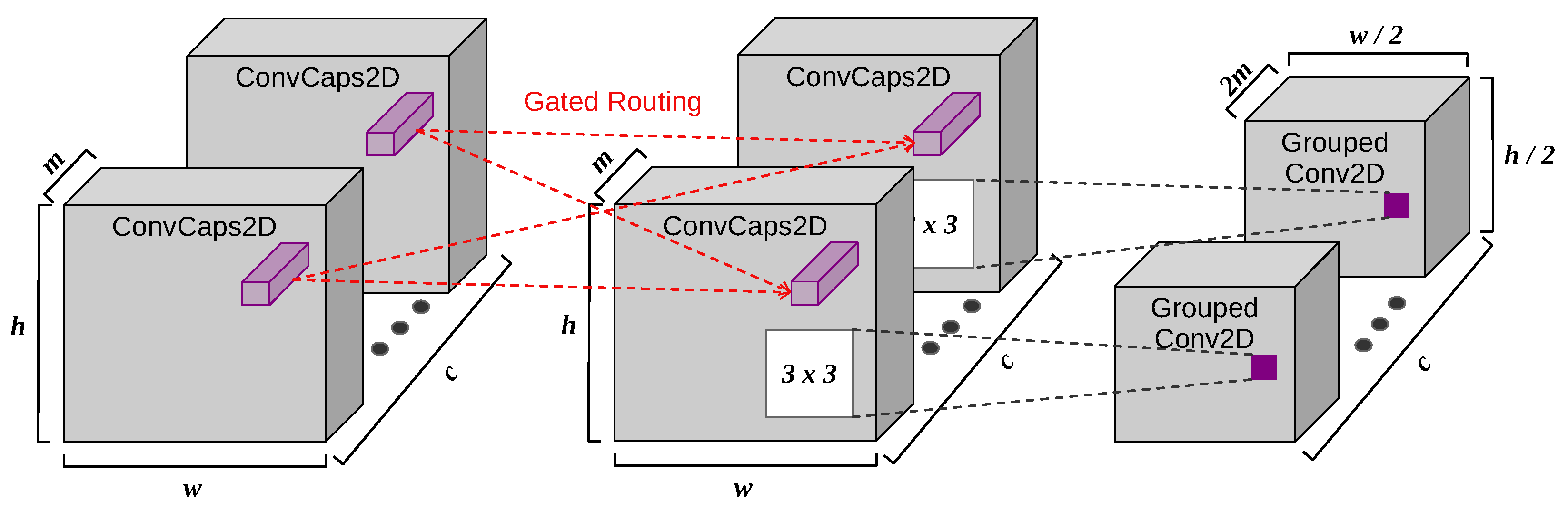
In our final experiment, we investigate the potential of a pure capsule-driven network with GR on the task of image classification. For this purpose, we apply a convolutional CapsNet on the datasets Fashion-MNIST and SVHN. In short, the network is composed of capsule-based feature maps with GR between feature maps of the same dimensionality, grouped convolutions [27] for downsampling feature dimensions, and 30 dense capsule blocks. Network scaling is modest in order to keep computation time feasible. A detailed architecture description can be found in Appendix C. To the best of our knowledge, this is the first pure capsule-driven architecture. Usually, capsules merely take place in the final two network layers of an extended net structure. We formulate the following research question:

RQ 7: 

Provide capsules the potential to embody arbitrary-level entities?

As a strategy against overfitting, dataset-specific data augmentation is used. The data augmentation for Fashion-MNIST includes horizontal flip ($p=0.5$), random zoom and translation with factors of $0.1$. The data augmentation for SVHN imitates the natural variances in the data using random zoom, translation and shear with factors of $0.1$. In addition, random rotation with a maximal magnitude of $5\%$ from $2\pi$ is employed. For each dataset, five randomly initialized CapsNets are trained over 100 epochs. The experimental results are illustrated in Figure 12 and

Table 10. Final training and test accuracies (in %) of the convolutional CapsNet on Fashion-MNIST and SVHN.

	Fashion-MNIST		SVHN
Set	Best	AVG	Best	AVG
Train	$86.11$	$85.77\pm 0.22$	$83.33$	$81.53\pm 1.97$
Test	$87.08$	$85.61\pm 1.02$	$86.59$	$85.38\pm 1.80$

.

RQ 7: The training and validation loss developments in Figure 12 point out that entirely capsule-oriented networks can operate on low-level and high-level entities. This is also supported by the adaptation of GR’s bias parameter similar to our previous results. However, our pure CapsNet does not achieve state-of-the-art test accuracy, as stated in Table 10. We attribute this deficit to CapsNets’ major limitation of intense computational complexity, resulting in long training sessions even for small architectures. We have the hope that future research into efficient routing algorithms and their low-level implementations will make CapsNets applicable to a broader range of machine-learning tasks.

5. Discussion

5.1. Remarks on the Degradation Problem

The experiments in this paper revealed that the degradation problem is versatile in its appearance. The most obvious form is degenerative performance with respect to model accuracy during inference and training. This aspect can be subdivided into global and local degenerative performance, whereas global refers to the average performance over several runs (including result variance) and local means the best-reached performance within multiple runs. For example, we found global degradation to be stronger for parametric activation functions; however, local degradation remains noticeably small with a gain in network depth. Another facet of the degradation problem regards the convergence behavior of the optimization process. We showed that without the application of AMSGrad (with Adam optimizer), the learning curves of deep nets tend to be fragile and often fail to converge at all. We also introduced the idea of information diffusion as a crucial risk factor to promote the degradation problem. In fact, our experimental results on plain networks at least indicate an entanglement between the kind and degree of nonlinearities with the magnitude of the degradation problem. Specifically, we hypothesize that GR’s adaptive signal selection mechanism helps to overcome the degradation problem by reducing the effective risk of information diffusion.

5.2. Increased Depth in Plain Nets

Similar to previous work [25,47], our empirical results confirm that the successful training of very deep feedforward nets can be realized with a deliberate network design and initialization. We found that initially biasing neural nets towards linear processing and the useful handling of salient gradients (here: Adam with AMSGrad) constitute universal ingredients for robust optimization of very deep networks. An outstanding insight of our experiments is the resistance of certain parametric activation functions (here: PReLU and D-PReLU) against the degradation problem despite several hundreds of layers. We attribute this ability to the disruptive re-forming of the loss function until the network is set in a proper condition.

5.3. Ensemble of Neural Processing Paths

In [24], the authors argued that residual networks with n units (i.e., layers) produce $O\left(2^n\right)$ implicit paths of neural information processing, which delivers a primary explanation for their gain in performance. We connect to this view by arguing that CapsNets, consisting of k capsules per layer and applying GR between consecutive layers can even amplify the positive effects on network performance by engendering $O\left(2^{nk}\right)$ implicit paths. Although ResNeXts theoretically yield the same number of implicit paths, their bottleneck structure after the residual parts impedes the selection of individual paths, especially at the time of network initialization.

5.4. Impact of Capsule Quantity

ResNeXts enhance classification accuracy by introducing grouped convolutions with an auxiliary dimension in network design, named cardinality and meaning the number of groups [27]. Grouped convolutions are inspired by the work [48] about dividing convolutional operations over multiple GPUs with subsequent merging in order to reduce memory requirements [27]. We ascribe the performance gain of grouped convolutions to their capsule-similar mechanics, where self-regularization occurs as restricted entity recognition per capsule (opposite to complete scene classification in the layers of plain nets) which results in stronger representations (cf. [27]). Thus, we equate cardinality with the number of capsules per layer and describe width as neuron count per capsule.

5.5. Computational Efficiency Considerations

In general, the integration of ANGs into a neural network potentially involves an additional parameter investment or increases the time complexity for optimization, resulting in longer training sessions. However, biased BN probably causes no auxiliary resource consumption in most cases because of its standard usage in very deep networks for preserving numerical stability. In the worst case BN adds one bias and scaling parameter per neuron to a network, whereas the bias parameters act as substitutes for the bias weights of neurons. The computational overhead induced by BN is negligible due to its beneficial impact on stable training. Using parametric activation functions as ANG realization, we observed a superior performance for low-parameterized variants like PReLU or D-PReLU. The parameter investment for these variants remains negligible, even in the useful combination with biased BN. The outcome of our experiments actually indicates that parametric activation functions can promote faster exploration of the solution space through their disruptive nature, leading to an accelerated optimization process. Despite GR’s reuse of transformation matrices, it requires extra $D\times N\times M$ bias parameters per layer for gating neuron signals where N and M correspond to the number of lower-layer and higher-layer capsules, respectively, and D means the neuron count per lower-layer capsule. An alternative option is the use of $N\times M$ parameters with only one bias weight per lower-layer capsule which could possibly mitigate overfitting issues. Note that CapsNets usually involve $D\times V\times N\times M$ weights for transformation matrices between two consecutive capsule layers, with V representing higher-layer capsule dimensionality. Although the additional parameter investment appears relatively high, comparable gating mechanisms for skip connection creation as in highway networks scale analogously. If SA is activated within GR we need to invest further $V\times M$ parameters per layer to select between incoming capsule signals. We argue that SA should be activated in the general case to mitigate noise accumulation over capsule layers. In comparison to regular routing algorithms such as DR and k-MR with their iterative computations, GR induces lower time complexity for signal propagation. Evidently, CapsNets generally suffer from higher computational efforts and often include more parameters in relation to plain neural networks but they also offer special properties for representation learning. Furthermore, CapsNets with self-building skip connections theoretically lead to a significant gain in implicit information processing paths compared to residual and highway networks. Thus, the choice of using CapsNets with self-building skip connections is determined by a trade-off between the needed representational capacity for a specific application task and the resulting computational efficiency.

5.6. Limitations of Our Empirical Study

The present paper serves as an introductory work for enabling the successful training of enlarged CapsNets by facilitating the learning of self-building skip connections. For this purpose, we provide ANG strategies for stabilizing the optimization process of very deep networks to effectively mitigate the degradation problem. Although we conducted a comprehensive experimental analysis to validate our theoretical framework and proposed methods, there are several limitations of our empirical study that restrict the scope of our work. At first, our experiments are limited to neural networks with extended depths but small neuron counts per layer to keep memory and computational efforts minimal. For obtaining meaningful results, most of the experiments were applied on the simple MNIST dataset. Note that the use of simple datasets especially intensifies the degradation problem by magnifying the overparametrization of our models with extended depths. Thus, the empirical results are sufficient for proving the preservation of a stable optimization process referring to training curves and accuracy but lack a state-of-the-art performance comparison with specialized models for more complex datasets and a broad range of application tasks. Specifically, we categorize our proposed approaches as complementary techniques to enhance existing state-of-the-art models, and to contribute to the understanding of the dynamics in very deep networks. In GR we involved a softmax temperature hyperparameter for enhanced control over the selectivity for incoming capsule signals. We hypothesize that the importance of the softmax temperature increases with the capsule count per layer. Since we used very deep but narrow CapsNets in our experiments, we kept the softmax temperature constant with a value of one. However, a proper hyperparameter search including other weight initialization schemes is recommended in the future investigation of advanced CapsNet models with state-of-the-art performance.

5.7. Future Research Directions

Following the versatile results and the limitations of our empirical study we identify several aspects that need to be addressed in future research efforts. First of all, a straightforward next step is the integration of our proposed methods into existing state-of-the-art models and conducting sophisticated performance comparisons for individual application domains. Since we introduced the concept of ANGs as a necessary precondition to facilitate the forming of self-building skip connections, we also suggest a thoroughly theoretical analysis in future work that formalizes ANGs and systematically investigates their effects on the training stability of diverse neural architectures. Moreover, we limited our practical ANG realizations to biased BN and parametric activation functions. A promising research direction constitutes the design of other ANG realizations for various network types and application tasks. Although we supplied implicit evidence about the creation of self-building skip connections based on the model’s resistance against the degradation problem and visualized the controlled access of nonlinear capacities within very deep networks, we highly recommend the future development of objective metrics for quantifying the existence and effectiveness of skip connection mechanisms. We believe that such metrics could deliver valuable insights and significantly contribute to better model comparability in this field.

6. Conclusions

In this work, we systematically analyzed the impacts of the degradation problem on the training of very deep plain networks and CapsNets up to a depth of 500 fully-connected layers. Through the unification of residual and highway networks into CapsNets, we provide a theoretical basis for beneficial properties in neural architectures to overcome limitations on network depth. Moreover, we complement our abstract concepts such as ANGs with practical methods like initially-biased BN or parametric activation functions that can be easily integrated into arbitrary net structures for effectively mitigating the degradation problem. Finally, the promising empirical results with CapsNets using GR open the successful training of extended capsule-driven architectures, which hopefully motivates future research efforts in this direction.