Abstract
Accurate and timely traffic forecasting is an important task for the realization of urban smart traffic. The random occurrence of social events such as traffic accidents will make traffic prediction particularly difficult. At the same time, most of the existing prediction methods rely on prior knowledge to obtain traffic maps and the obtained map structure cannot be guaranteed to be accurate for the current learning task. In addition, traffic data is highly non-linear and long-term dependent, so it is more difficult to achieve accurate prediction. In response to the above problems, this paper proposes a new integrated unified architecture for traffic prediction based on heterogeneous graph attention network combined with residual-time-series convolutional network, which is called HGA-ResTCN. First, the heterogeneous graph attention is used to capture the changes in the relationship between the traffic graph nodes caused by social events, so as to learn the link weights between the target node and its neighbor nodes; at the same time, by introducing the timing of residual links convolutional network to capture the long-term dependence of complex traffic data. These two models are integrated into a unified framework to learn in an end-to-end manner. Through testing on real-world data sets, the results show that the accuracy of the model in this paper is better than other proposed baselines.
1. Introduction
In recent years, with the continuous development of society, how to build a complete smart transportation system has become an important research area [1], because smart transportation systems can improve traffic efficiency and make transportation decisions quickly. Traffic data prediction based on urban traffic road network is the main research direction. Accurate traffic prediction can not only solve clear traffic tasks, but also reflect the traffic conditions on the road, middle and downstream in a timely manner [2,3,4].
In the urban traffic road network, a large number of traffic sensors are used, so there is a large amount of historical traffic data in the traffic system. In this dynamically changing traffic system, there must be a wealth of traffic network information and road relationship information hidden in the data. Most of the early researchers used classical statistical methods to predict the traffic data of a single point or a single lane. Among them, the methods used are Markov chain [5], ARIMA model [6] and its variant subsets ARIMA [7] and seasonal ARIMA [8], etc., but the disadvantage of these methods is that the conditional variance of the time series remains unchanged. Therefore, such a model is not very useful in real traffic forecasting; later appeared one after another. Many data-driven algorithms, such as Bayesian networks and neural networks [9], SVM [10], KNN [11], etc., but these algorithms are flawed under dynamic traffic conditions because they cannot capture the height of traffic data, as well as non-linear spatial-temporal characteristics, and cannot be applied to a large number of data sets.
In recent years, many researchers have used deep learning-based methods to predict traffic, mainly identifying and extracting complex features of traffic data, such as GRU [12], LSTM [13], but these have ignored the importance of traffic data Spatial dependence; later, some frameworks mixed with convolutional neural networks (CNN) were proposed to capture the complex spatial-temporal correlation of traffic data [14,15], but CNN is usually suitable for processing traffic data of graph or regular network in traffic data prediction, and cannot work under the complex urban road network, so the traffic data cannot be processed as a regular grid format tensor.
Most recent researches express traffic prediction as a problem of graphical modeling. Yu, Yin and Zhu et al. [4] proposed a deep learning framework called Spatial-Temporal Graph Convolutional Network (STGCN), which can more accurately extract the spatial-temporal correlation between connected nodes, but the graph convolution in the model cannot clearly describe the various transmission modes between nodes, and do not take into account the changes in the relationship between nodes in the traffic graph. Wu, Pan et al. [16] proposed a graph wave network combined with GCN to deal with the temporal and spatial correlation of road networks. The proposed adaptive adjacency matrix can automatically learn the hidden spatial relationships between traffic data, but the model will be too smooth and cannot be resolved; Guo, Lin [17] proposed an attention-based spatial-temporal graph convolutional network (ASTGCN) model to solve the traffic prediction problem; Song et al. [18] proposed a new spatial-temporal synchronization graph convolutional network (STSGCN) model for spatial-temporal network data prediction, and a number of modules in different time periods are designed in the model, In order to effectively capture the heterogeneity in the local spatial-temporal graph, Hu et al. [19] proposed a new traffic prediction dynamic graph convolutional network, by introducing a latent network to extract spatial-temporal features, constructing a dynamic road network graph matrix.
In these recent studies, although they use graph convolutional networks and add corresponding spatial-temporal mechanisms to capture the dynamic correlation of traffic data, these methods rely on prior knowledge to obtain the graph structure, and the obtained graph structure cannot ensure that the current learning task is accurate, and the predefined graph structure is generally fixed, and the defined graph structure will not be changed [20]; at the same time, considering the random occurrence of social events such as traffic accidents, it will lead to changes in the relationship between nodes in the traffic network graph. Therefore, it is difficult to model the dynamics of traffic data using a fixed graph structure; moreover, in the real world, traffic data recorded by sensors on traffic roads are generally for long-term dependence; the use of the aforementioned RNNs will be very time-consuming, so the long-term dependence of traffic data cannot be accurately captured. Therefore, we need a new method to solve it.
In this work, we propose a new deep learning traffic prediction integrated framework based on heterogeneous graph attention network combined with residual-time-series convolutional network, which solves the two shortcomings mentioned in this article, and the model can automatically change from the temporal and spatial characteristics of dynamic changes between traffic data are learned in the road network. Specifically, the graph attention layer learns the relationship between changes in roads caused by random social events, and maps the changed node features to the same feature space through a transformation matrix. The purpose is to learn the target node with the new weight change coefficient between its neighbors, and finally re-aggregate the features of the neighbors hierarchically to form the node embedding of the network to capture the spatial dependence between the traffic data; using the time series convolutional network that introduces the residual link to capture the traffic for the time dependence between data, a residual block is constructed to replace the convolution operation of one layer. Among them, a residual block contains a nonlinear mapping and a two-layer convolution operation. Each layer adds dropout to regularize the network, so it is helpful to improve the calculation and can solve the complicated long-term dependence between traffic data. The two parts are integrated to model the complex spatial-temporal correlation of traffic data. The main contributions of this work are as follows:
- This paper proposes a new integrated unified framework called HGA-ResTCN to capture the temporal and spatial correlation of traffic data in an end-to-end manner. The core idea is to model and capture changes in the relationship between urban traffic and roads caused by the random occurrence of social events such as traffic accidents in the process of traffic prediction.
- Introducing the residual-time-series convolutional network into traffic prediction make it easier to capture long-term dependencies between traffic data. Contrary to the method based on RNNs, the time network designed in this way has more generalization ability and can correctly process long-term dependent time series in a non-recursive manner, which is beneficial to parallel computing and speeds up the training time of the network.
- The HGA-ResTCN model is evaluated on the real-world data set PEMS-BAY, and its accuracy is better than other proposed baselines.
The rest of this article is arranged as follows. Section 2 introduces some problems of traffic forecasting and the related definitions of this article. The third section introduces the model architecture system of this article. The fourth section is the experimental part. The fifth section is a summary of work and future prospects.
2. Related Work
2.1. Traffic Forecast
Traffic prediction is essentially a complicated time series forecasting problem. It predicts the future traffic data of the target road section through the current and past observed traffic data in the traffic road network [16], but due to the highly non-linearity of the traffic data, Randomness, and long-term dependence, etc., the predictive models as mentioned above usually perform poorly. At the same time, social events such as traffic accidents that occur randomly on the roads will inevitably lead to changes in the relationship between the roads. In the work of this article, we define that the nodes of the traffic graph are connected by path , . Therefore, the input data of the i-th road node based on the path pi at time t is , i = 1, 2, …, N, where N is the number of road nodes, is the type of characteristic size. For example, f = 2 means that our model will accept two different types of road traffic data. Therefore, the traffic data of the road network based on the path P at time t is expressed as , Therefore, the input data is ; we use Q-step input data to predict the future traffic data from step 1 to step M, and the predicted result is in order to process multidimensional traffic data; the integrated model in this paper can capture the complex spatial-temporal relationship between multiple inputs and outputs, especially the transfer characteristics of traffic data in time and space, which can be integrated into the model to improve the performance of traffic prediction and can reduce the randomness of the data.
2.2. Graph Attention Network
Since the attention mechanism has a relatively good performance in the correlation between learning signals, some researchers have introduced the attention mechanism into the deep convolution model, automatic coding learning and generation network, and achieved relatively good performance [21,22]. After that, the researchers proposed a self-attention mechanism [22]; the purpose is to show the characteristics of the data or the interdependence between the input signals in a mathematical form. Compared with the self-attention mechanism, another attention method [23] was subsequently proposed. Its mechanism is to calculate the relationship between different types of features through a weighting matrix, and the weighting coefficients of different features are different. In recent years, the graph attention network [24] appeared. It was the first to use the attention mechanism and neural network to adapt learn the dynamic adjacency matrix of the graph, and achieved satisfactory results in semi-supervised learning tasks performance. We take the heterogeneous graph attention network into consideration in traffic prediction to deal with and adapt to the proposed problems and scenarios. The attention mechanism in it can deal with changes in the relationship between nodes, and can effectively capture and describe road nodes’ changes in the relationship. In this work, before aggregating the neighbor information of each target node, it should be noted that neighbor nodes affected by sudden factors will show different importance relative to the target node in the node embedding learning, and thus show a different relationship. In this article, the HGA module’s own attention mechanism can learn the importance of neighbor nodes to the target node, and re-aggregate the representations of its neighbors to form node embedding.
Preliminary
We define the road network as a heterogeneous graph , It is composed of node set V and edge set E, where . The edge set E is represented by the set of defined path ; It is to show that under the influence of sudden social events, road nodes will have different influence relationships between nodes. This article only considers the weights of undirected graph network nodes. The purpose of traffic prediction is to learn a function from historical traffic data of Q steps. The N road sensors on the road network predict the future traffic data from 1 step to M steps.
3. Methodology
In this section, we will introduce the overall framework of this article and the models of each part in detail, including the heterogeneous graph attention network module and the residual time series convolutional network module.
3.1. Overall Framework
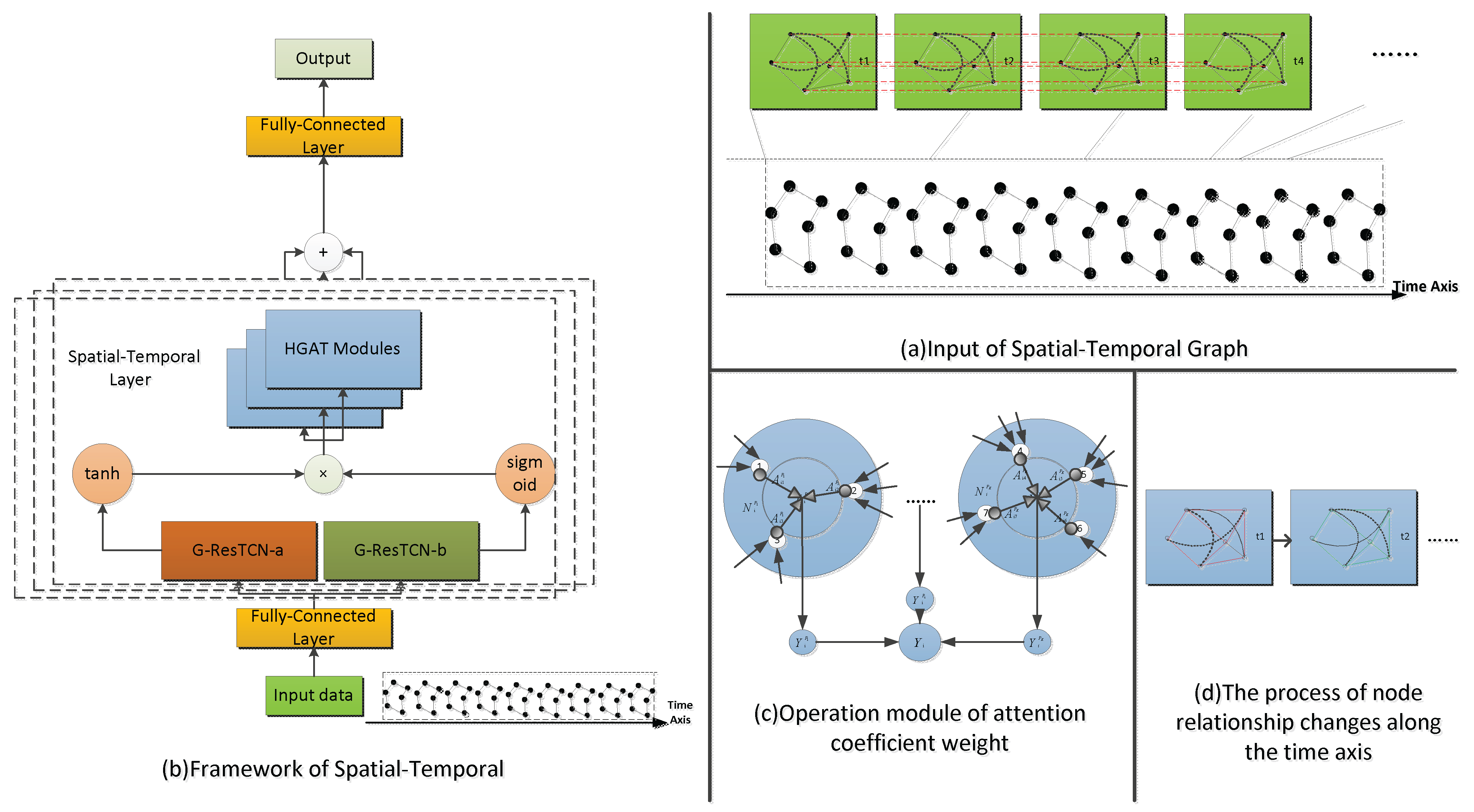
The overall framework of the end-to-end HGA-ResTCN model is introduced in Figure 1b below. It is composed of a data input layer, a stacked space-time layer, and an output layer. The input layer and the output layer are one fully connected layer. The space-time layers of each stacked layer are composed of several parallel layers. The HGAT module is composed of two parallel gated-residual timing convolutional network modules, which are respectively responsible for capturing the spatial and temporal characteristics of traffic data. By stacking several spatial-temporal layers, nodes can obtain information between higher-order neighbors in a hierarchical manner. More importantly, the HGA-ResTCN model can capture the spatial-temporal traffic information after the relationship between nodes has changed.
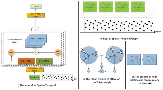
Figure 1.
HGA-ResTCN framework: (a) An example of input for our spatial-temporal graph, the purpose is to show the relationship between different graph nodes, and use the traffic information features on the graph as input to our model. (b) For our time-space framework, input data X, including map information features and traffic features observed by each sensor (such as traffic speed, occupancy rate, etc.); Among them, the use of two parallel gating mechanisms is to expand the receiving domain of the network, thereby enhancing the performance of the model to extract long-term dependencies between traffic data; and each layer model of the stacked heterogeneous graph attention module will receive independent training and jointly extract the spatial dependence of mutual influence between graph nodes. The two parts together constitute the spatial-temporal layer of the model, which is used to extract the spatial-temporal characteristics of traffic data. (c) is the specific representation module of the change of the attention weight coefficient of the heterogeneous graph attention module. (d) is the process diagram of the node relationship changing over time. The thickness of the dashed line and the color of the edge in the figure indicate the change process of the node relationship.
3.2. Heterogeneous Graph Attention Module
The function of each HGAT module is to dig out the spatial dependence of the traffic data after the node relationship of the traffic network graph has changed.
In order to clearly describe the module, first, we define a transformation matrix based on the changed road node relationship. It is a matrix composed of different node connection relationships. Its elements are only 1 and 0, indicating whether there is a connection relationship between nodes. The transformation matrix contains static node connection relationships, and through the next step of mapping transformation, can be used to transfer the changed node state relationship; in the case of a given node feature as an input, map the different types of road node features after the change to the same feature space. For example, the mapping formula for type nodes is as follows:
where, is the feature matrix of the original data, and is the feature matrix of the mapped data. Through mapping, any neighbor nodes with different importance to the target node can be processed, and at the same time, the mapping calculation is changing with the time, the node, and the change of the node relationship.
Subsequently, self-attention is used to learn the weights between nodes. Given a node pair (i, j) connected by path link , the calculation formula for the importance of node j to node i is:
where, is a deep neural network that calculates attention. is asymmetric; that is, the importance of node i to node j is different from the importance of node j to node i [25]. Then we introduced the graph structure information into the mechanism by shielding attention, and normalized it with soft-max to obtain the attention weight coefficient learned by . The calculation formula is:
The attention weight coefficients of the node pair (i, j) completely depend on their own changing characteristics. is asymmetric, which means that they contribute differently to each other, not only because the molecular connection order in the normalization calculation is different, but also because they have different neighbor nodes, the denominator in the normalization calculation will also be very different. Figure 1c represents the specific operation of the attention weight coefficient. The embedding of node i can be aggregated by the mapping features of its neighbors and its attention weight coefficient, which is expressed as:
Among them, is defined as the neighbor node set of node i based on the path link . In the case of a given link , each target node has a set of neighbor node sets containing its own node, which can show the structure of different node relationships. information. And because of the high complexity and dynamics of traffic data, we need to pay attention to and capture more changes in the relationship between nodes; at the same time, in order to train more stable and increase the expressive ability of the attention mechanism, we will use multi-head attention, which means for:
Among them, C is the adjustable number of multi-head attention. Multi-head attention can make the parameter matrix form multiple subs-paces, which are multiple independent attention calculations, and the overall size of the matrix is unchanged, but the dimension corresponding to each head is changed, so that the matrix can be used for multiple different nodes. The mutual influence relationship between the two is studied, and the amount of calculation is equivalent to that of a single head. Finally, according to different data and different path links, K groups of embedding can be obtained, which are aggregated to form network embedding to jointly learn the changing spatial dependencies between traffic data.
3.3. Residual-Time Series Convolutional Network Module
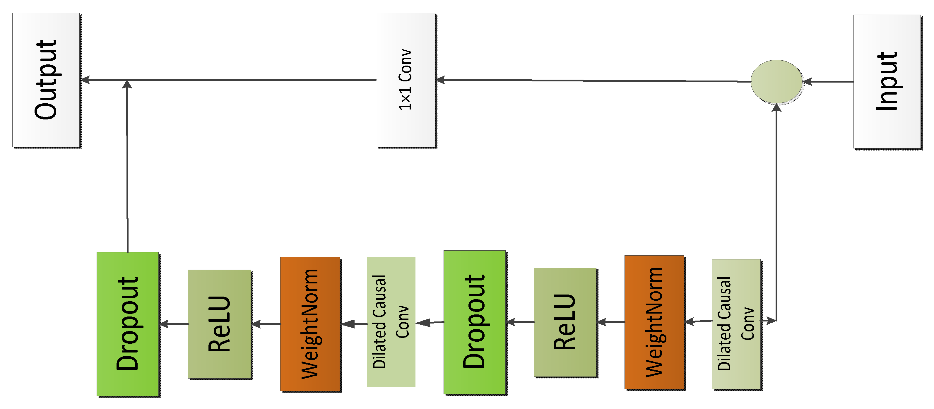
In this paper, a time-series convolutional network [26] with residual link is used to capture the time dynamics of traffic data. Some researchers generally use cyclic neural networks and their network variants for modeling time series [12]. This is because cyclic neural networks have a cyclic auto regressive structure that can capture the differences between time series well. Contrary to the method based on RNNs, this article adopts a general temporal convolutional network (TCN) architecture that is suitable for all tasks. Among them, the dilated causal convolution in TCN preserves the causal order of the time series by filling zeros into the input, so the prediction on the current time step only involves historical information [16]. Therefore, the TCN architecture is not only more accurate than general recursive networks (such as LSTM and GRU), but also has a simpler structure. More importantly, it requires less memory during training, especially for long input time series. Therefore, the long-term dependency between traffic data can be accurately captured. Given the input of a one-dimensional time series and a filter , as shown in Figure 2 below, the causal convolution operation of the time series and the filter is:
where d is the expansion factor and K is the filter size.

Figure 2.
TCN residual block. The 1 × 1 convolution is added when the input and output sizes of the residual block are not the same.
Residual link: A residual block [27] contains a link that leads to a transformation function F, and the subsequent output will be added to the input x of the residual block. This operation can effectively allow each layer to learn pairs the modification of the mapping can effectively improve the calculation speed without learning the conversion process of the entire network. It is expressed as:
Gating mechanism: The role of gating mechanism is particularly important in recurrent neural networks. The researchers said that the gating mechanism plays an important role in controlling the information of each layer in the time convolutional network [28]. The gating mechanism used in this article is expressed as:
Among them, and are two activation functions respectively, and are two independent convolution operations, and are model parameters, is the element-wise product, and the introduction of a gating mechanism is to expand the reception of the network layer domain to enhance model performance and extract long-term dependencies between traffic data [29].
4. Experiment
This section uses real-world traffic data sets to evaluate the proposed model, and its performance is better than the proposed baseline.
4.1. Data and Settings
We trained and tested using the PEMS-BAY dataset collected from the California Gulf Area Transportation Department and the METR-LA dataset collected from loop detectors on the Los Angeles County Highway.
The PEMS-BAY dataset contains six speed information recorded by 325 sensors from 1 January 2017 to 31 May 2017. In this dataset, data were collected every 5 min. with a number of 2369 edges and a deletion rate of 0.003%. Among them we screened out 90 sensor data with significant changes in speed over a time period as experimental data for the innovative section.
The METR-LA dataset ranged from March 2012 to June 2012, recording 207 sensors (nodes) on the Los Angeles County Highway, 1515 edges with time steps of 34,272, a data loss rate of 8.109% and 4-month traffic.
Both data-sets were processed the same, both dividing data-sets in chronological order, with 70% for training, 20% for testing and 10% for validation. The data input length is set to 12 (equivalent to one hour of collected data). In the training phase, batch size = 32, learning rate Ir = 0.001, and epoch = 150. The architecture of the code is Pytorch, and experiments were conducted on a server computer with Tesla V100 32G GPU and Lenovo i7-10700 CPU.
4.2. Baseline
HA: The historical average model [30].
ARIMA: Auto regressive integrated moving average model [6].
FC-LSTM: Fully connected LSTM, a variant of LSTM with input and hidden state in vector form [30].
STGCN: Spatial-Temporal graph convolutional networks composed of graph convolutional layers and convolutional sequence learning layers [4].
STSGCN: Spatial-Temporal synchronous graph convolutional networks [18].
DCRNN: Diffusion convolutional recurrent neural network: Data-driven traffic forecasting [2].
4.3. Evaluation Index
There are two evaluation indicators used in this article. We take the root mean square error (RMSE) and mean absolute error (MAE) and average absolute percentage error (MAPE) between the predicted value and the actual value in the real world as the loss function of the model, and pass it back propagation during training. Missing values are excluded both from training and testing. To minimize it as much as possible, it is defined as follows:
4.4. Accuracy and Performance Comparison
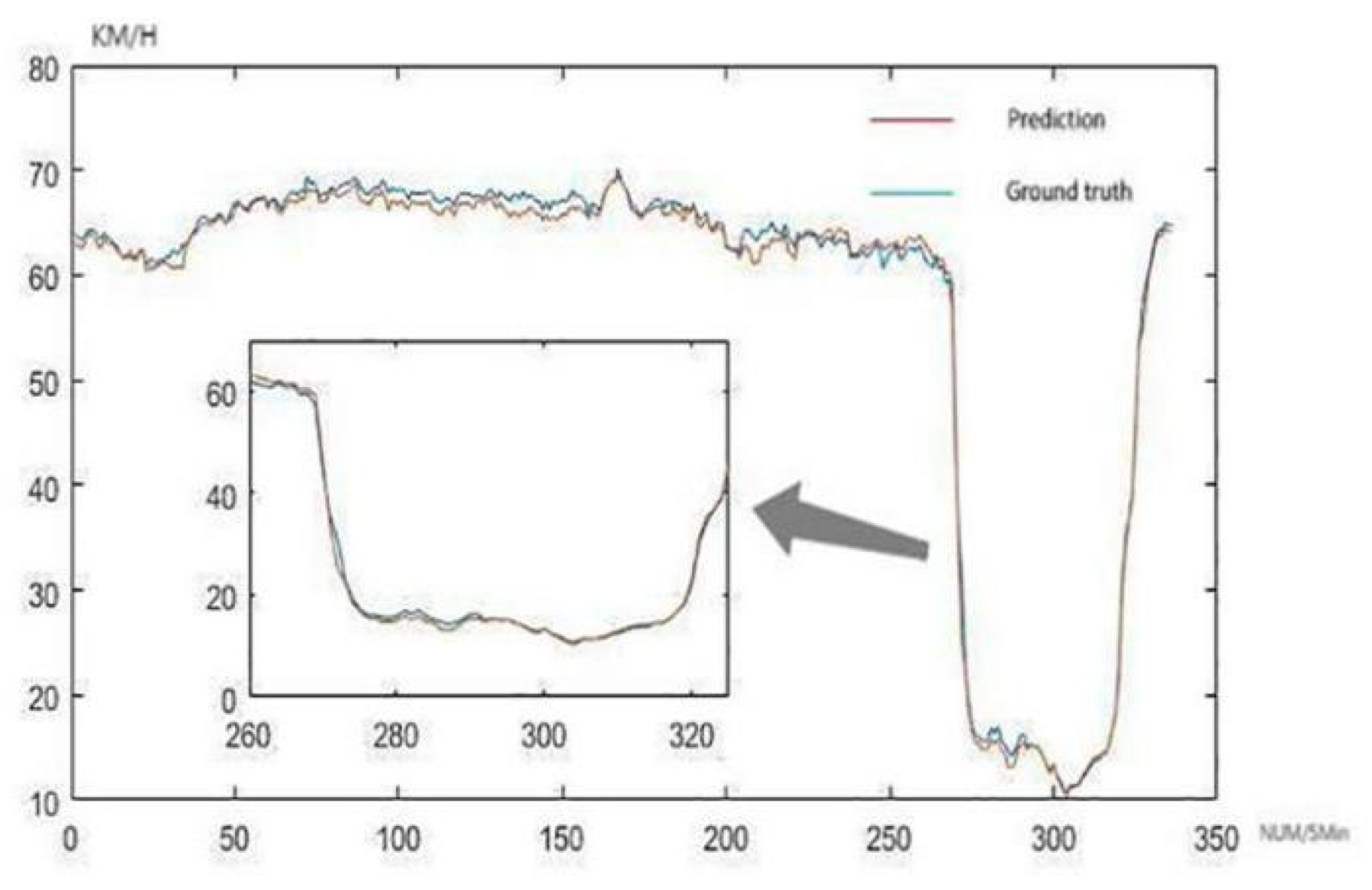
The performance of the different models and the comparison results of the present model are shown in Table 1 and Table 2 below. We evaluated all model baselines to predict the traffic speed in the next 15 min, 30 min, and 60 min. It can be seen that the performance of the HGA-ResTCN model in short-term and medium-term traffic speed prediction is better than the other baselines given, especially in the short-term speed prediction, the accuracy improvement is relatively large. The model corresponding to Constant-HGA-ResTCN has the same structure as HGA-ResTCN, but the difference is that it has a constant attention mechanism (the same attention weight coefficient is assigned to each neighbor node), so only the relationship between fixed nodes can be captured. Although models such as STSGCN can also extract the temporal and spatial dependence of traffic speed through graph convolution combined with time modules, the HGA-ResTCN model has obvious advantages over other models in capturing changes in node relationships. The Figure 3 below also shows the prediction results of 336 time points on a certain sensor. It can be seen that the HGA-ResTCN model is superior in capturing changes in the node relationship.

Table 1.
The PEMS-BAY dataset comparison with other baselines in the next 15, 30 and 60 min.

Table 2.
The METR-LA dataset comparison with other baselines in the next 15, 30, and 60 min.
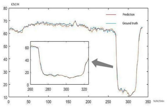
Figure 3.
Traffic prediction and the corresponding ground truth of a sensor during 336 time points.
4.5. Selection of Model Hyper Parameters
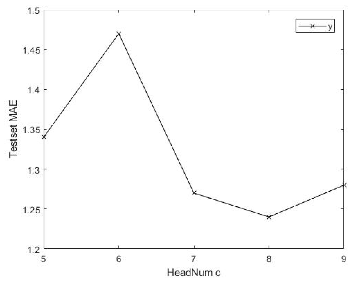
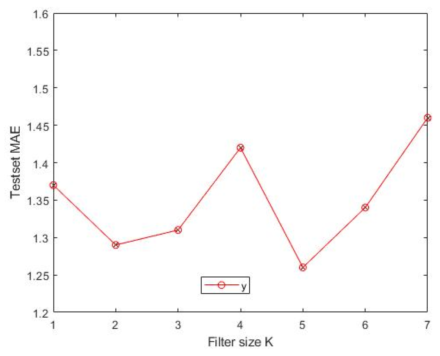
The hyper parameters to be determined in the model include the size of the time convolutional network filter and the number of multi-head attention mechanisms, which respectively correspond to the relevance of the change in the relationship between the receiving domain and the nodes. The amount of multi-head attention will directly affect the performance of the HGA-ResTCN model. At the same time, a larger filter allows the time module to capture wider time dependence. The Figure 4 and Figure 5 below shows the change of the MAE on the test data set with the number of hyper parameters c and K. It can be clearly seen that when c = 8 and K = 5, the performance of the model is evaluated on the test set. The MAE reached the minimum value.
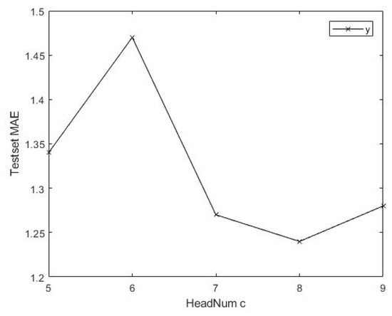
Figure 4.
Effects of c.
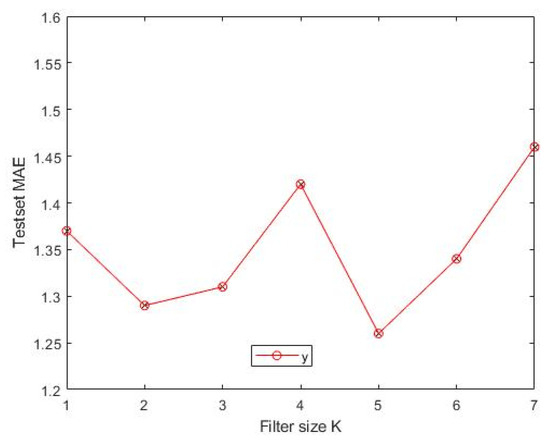
Figure 5.
Effects of K.
4.6. Advantages of Introducing a Multi-Head Attention Mechanism
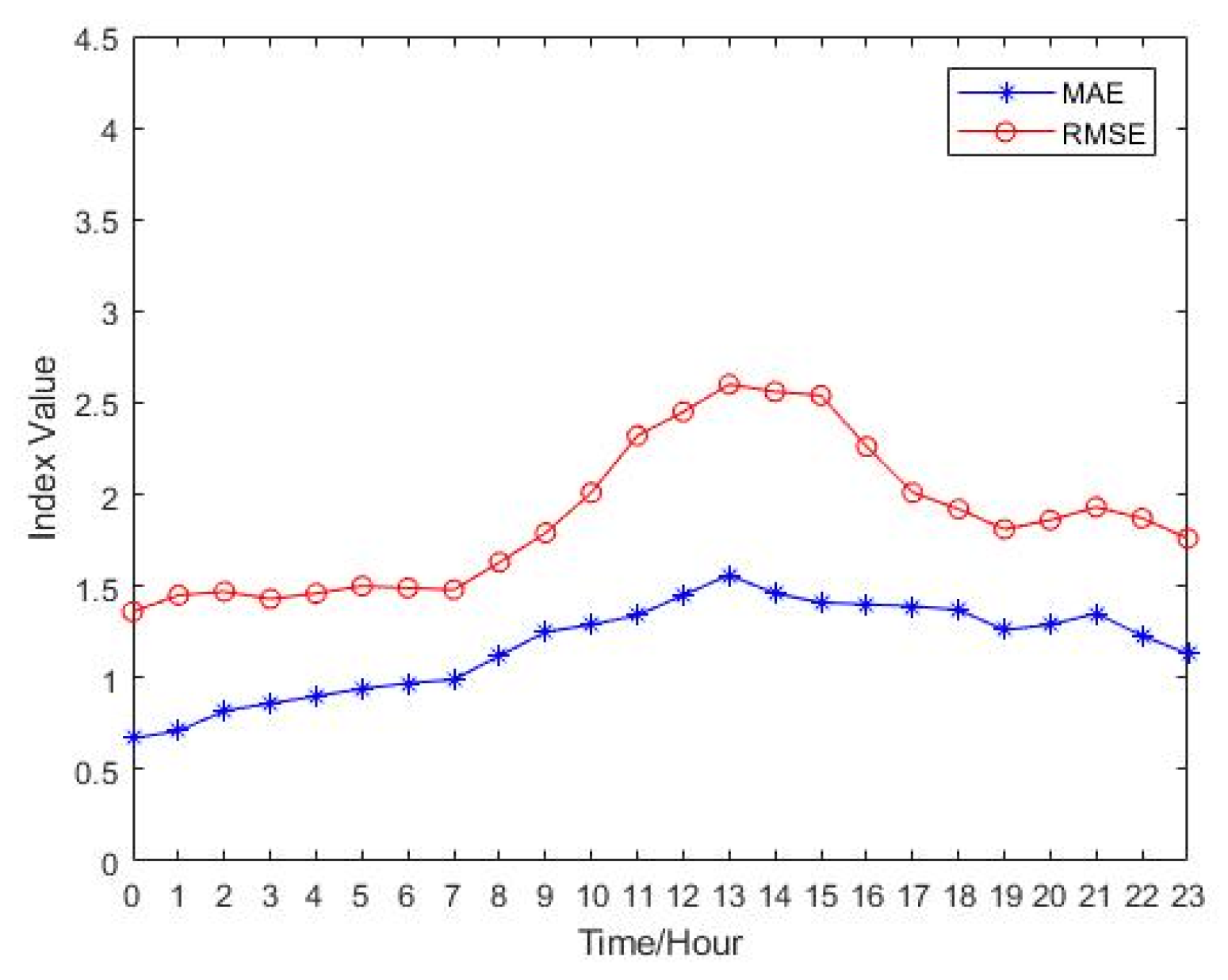
The following Figure 6 shows the changes of the two indicators we evaluated during the day. It can be seen that the values of these two indicators have changes at the peak. The rest of the time is relatively stable and has a similar pattern, while the changes at the peak are due to the occurrence of emergencies; changes in traffic speed within a short period of time cause changes in the relationship between road nodes, but it is relatively stable in the rest of the time. This is also attributed to the use of multi-headed attention in the HGA-ResTCN model. Explore more changes in the relationship between nodes and enable the model to maintain a relatively stable performance state for the rest of the day.
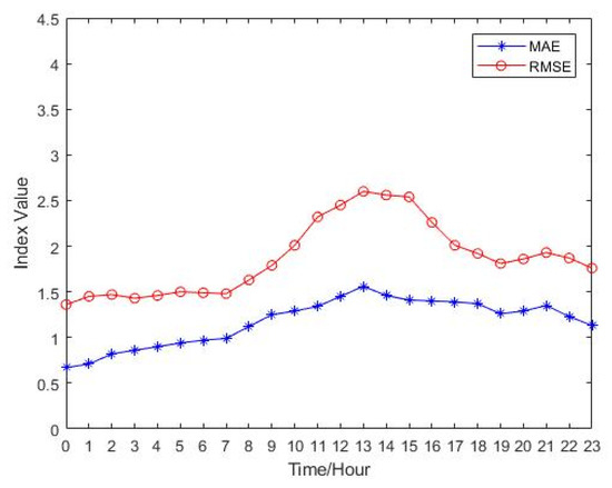
Figure 6.
Two indicators evaluated on one day’s test data set.
4.7. Visualizing Attention Correlation Coefficient
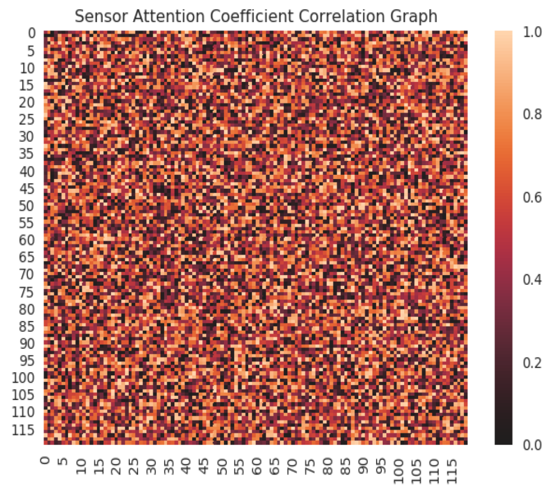
Figure 7 shows the attention coefficient matrix of the first HGAT layer with heat maps of different colors. The X-axis and Y-axis refer to 120 sensors sampled from PeMS-BAY traffic data. The pixel value at point (x, y) represents the correlation coefficient between the two sensors, and the depth of the pixel represents the correlation between the corresponding two sensors. However, due to the initial training stage, the attention correlation coefficient is relatively small, so the heat map looks more uniform. The attention coefficient matrix is the key to the spatial correlation of traffic prediction modeling, so that the HGA-ResTCN model can better capture the characteristics of changes in the relationship between nodes.

Figure 7.
Sensor attention correlation coefficient heat map.
5. Conclusions
This paper proposes a heterogeneous graph attention-residual time series convolutional network for multi-step prediction of traffic speed. Aiming at the problem of dynamic changes in the relationship between traffic and roads affected by social events such as traffic accidents, the method proposed in this paper is proven it has good performance to extract the spatial-temporal correlation of this dynamic change of traffic data. This method is evaluated on real-world traffic data sets. The experimental results show that the method in this paper is superior to other proposed traffic prediction methods. However, if we want to predict the traffic data of a large-scale road network in the future, it is a critical and complex task to consider the changing relationship between the target road and the higher-order roads adjacent to it.
Author Contributions
Conceptualization, Y.D. and K.Y.; methodology, Y.D.; software, Y.D.; validation, Y.D.; investigation, Y.D.; writing—original draft preparation, Y.D.; writing—review and editing, X.Q.; supervision, M.L.; project administration, X.Q., Z.J. All authors have read and agreed to the published version of the manuscript.
Funding
This research received no external funding.
Conflicts of Interest
The authors declare no conflict of interest.
References
- Snyder, C.; Do, M. Streets: A novel camera network dataset for traffic flow. Adv. Neural Inf. Process. Syst. 2019, 32, 10242–10253. [Google Scholar]
- Li, Y.; Yu, R.; Shahabi, C.; Liu, Y. Diffusion convolutional recurrent neural network: Data-driven traffic forecasting. In Proceedings of the Sixth International Conference on Learning Representations (ICLR), Vancouver, BC, Canada, 30 April–3 May 2018. [Google Scholar]
- Bai, L.; Yao, L.; Kanhere, S.S.; Wang, X.; Sheng, Q.Z. Stg2seq: Spatial-temporal graph to sequence model for multi-step passenger demand forecasting. In Proceedings of the 28th International Joint Conference on Artificial Intelligence, Macao, China, 10–16 August 2019; pp. 1981–1987. [Google Scholar]
- Yu, B.; Yin, H.; Zhu, Z. Spatio-temporal graph convolutional networks: A deep learning framework for traffic forecasting. In Proceedings of the 27th International Joint Conference on Artificial Intelligence, Stockholm, Sweden, 13–19 July 2018; pp. 3634–3640. [Google Scholar]
- Qi, Y.; Ishak, S. A hidden markov model for short term prediction of traffic conditions on freeways. Transp. Res. Part C Emerg. Technol. 2014, 43, 95–111. [Google Scholar] [CrossRef]
- Ahmed, M.; Cook, A. Analysis of freeway traffic time series data by using Box-Jenkins techniques. Transp. Res. Rec. 1979, 773, 1–9. [Google Scholar]
- Lee, S.; Fambro, D.B. Application of subset autoregressive integrated moving average model for short-term freeway traffic volume forecasting. Transp. Res. Rec. 1999, 1678, 179–188. [Google Scholar] [CrossRef]
- Williams, B.M.; Hoel, L.A. Modeling and forecasting vehicular traffic flow as a seasonal arima process: Theoretical basis and empirical results. J. Transp. Eng. 2003, 129, 664–672. [Google Scholar] [CrossRef] [Green Version]
- Sun, S.; Zhang, C.; Yu, G. A bayesian network approach to traffic flow forecasting. IEEE Trans. Intell. Transp. Syst. 2006, 7, 124–132. [Google Scholar] [CrossRef]
- Hong, W.C. Traffic flow forecasting by seasonal SVR with chaotic simulated annealing algorithm. Neurocomputing 2011, 74, 2096–2107. [Google Scholar] [CrossRef]
- Chang, H.; Lee, Y.; Yoon, B.; Baek, S. Dynamic near-term traffic flow prediction: System-oriented approach based on past experiences. IET Intell. Transp. Syst. 2012, 6, 292–305. [Google Scholar] [CrossRef]
- Xu, J.; Rahmatizadeh, R.; Bölöni, L.; Turgut, D. Real-time prediction of taxi demand using recurrent neural networks. IEEE Trans. Intell. Transp. Syst. 2017, 19, 2572–2581. [Google Scholar] [CrossRef]
- Tian, Y.; Zhang, K.; Li, J.; Lin, X.; Yang, B. LSTM-Based traffic flow prediction with missing data. Neurocomputing 2018, 318, 297–305. [Google Scholar] [CrossRef]
- Ke, J.; Zheng, H.; Yang, H.; Chen, X.M. Short-term forecasting of passenger demand under on-demand ride services: A spatiotemporal deep learning approach. Transp. Res. Part C Emerg. Technol. 2017, 85, 591–608. [Google Scholar] [CrossRef] [Green Version]
- Ma, X.; Dai, Z.; He, Z.; Ma, J.; Wang, Y. Learning traffic as images: A deep convolutional neural network for large-scale transportation network speed prediction. Sensors 2017, 17, 818. [Google Scholar] [CrossRef] [PubMed] [Green Version]
- Wu, Z.; Pan, S.; Long, G.; Jiang, J.; Zhang, C. Graph wavenet for deep spatial-temporal graph modeling. In Proceedings of the 28th International Joint Conference on Artificial Intelligence, Macao, China, 10–16 August 2019; pp. 1907–1913. [Google Scholar]
- Guo, S.; Lin, Y.; Feng, N.; Song, C.; Wan, H. Attention based spatialtemporal graph convolutional networks for traffic flow forecasting. In Proceedings of the AAAI Conference on Artificial Intelligence, Honolulu, HI, USA, 27 January–1 February 2019; Volume 33, pp. 922–929. [Google Scholar]
- Song, C.; Lin, Y.; Guo, S.; Wan, H. Spatial-Temporal Synchronous Graph Convolutional Networks: A New Framework for Spatial-Temporal Network Data Forecasting. In Proceedings of the AAAI Conference on Artificial Intelligence, New York, NY, USA, 7–12 February 2020; Volume 34, pp. 914–921. [Google Scholar]
- Guo, K.; Hu, Y.; Qian, Z.; Sun, Y.; Gao, J.; Yin, B. Dynamic Graph Convolution Network for Traffic Forecasting Based on Latent Network of Laplace Matrix Estimation. IEEE Trans. Intell. Transp. Syst. 2020, 1–10. [Google Scholar] [CrossRef]
- Diao, Z.; Diao, Z.; Wang, X.; Zhang, D.; Liu, Y.; Xie, K.; He, S. Dynamic Spatial-Temporal Graph Convolutional Neural Networks for Traffic Forecasting. In Proceedings of the AAAI Conference on Artificial Intelligence, Honolulu, HI, USA, 27 January–1 February 2019. [Google Scholar]
- Zhang, H.; Goodfellow, I.; Metaxas, D.; Odena, A. Self-Attention Generative Adversarial Networks. arXiv 2018, arXiv:1805.08318. [Google Scholar]
- Feng, X.; Guo, J.; Qin, B.; Liu, T.; Liu, Y. Effective deep memory networks for distant supervised relation extraction. In Proceedings of the 26th International Joint Conference on Artificial Intelligence, Melbourne, Australia, 19–25 August 2017; Volume 17, pp. 4002–4008. [Google Scholar]
- Velickovic, P.; Cucurull, G.; Casanova, A.; Romero, A.; Lio, P.; Bengio, Y. Graph attention networks. In Proceedings of the International Conference on Learning Representations, Vancouver, BC, Canada, 30 April–3 May 2018; pp. 1–5. [Google Scholar]
- Vaswani, A.; Shazeer, N.; Parmar, N.; Uszkoreit, J.; Jones, L.; Gomez, N.A.; Kaiser, L.; Polosukhin, I. Attention is All you Need. In Proceedings of the 2017 Conference on Neural Information Processing Systems, Long Beach, CA, USA, 4–9 December 2017; pp. 5998–6008. [Google Scholar]
- Bai, S.; Kolter, J.Z.; Koltun, V. An Empirical Evaluation of Generic Convolutional and Recurrent Networks for Sequence Modeling. arXiv 2018, arXiv:1803.01271. [Google Scholar]
- He, K.; Zhang, X.; Ren, S.; Sun, J. Deep residual learning for imag recognition. In Proceedings of the IEEE Conference on Computer Vision and Pattern Recognition, Las Vegas, NV, USA, 27–30 June 2016. [Google Scholar]
- Dauphin, Y.N.; Fan, A.; Auli, M.; Grangier, D. Language modeling with gated convolutional networks. In Proceedings of the 2017 International Conference on Machine Learning, Sydney, Australia, 6–11 August 2017; pp. 933–941. [Google Scholar]
- Li, M.; Zhu, Z. Spatial-Temporal Fusion Graph Neural Networks for Traffic Flow Forecasting. arXiv 2021, arXiv:2012.09641. [Google Scholar]
- Liu, J.; Guan, W. A summary of traffic flow forecasting methods. J. Highw. Transp. Res. Dev. 2004, 3, 82–85. [Google Scholar]
- Sutskever, I.; Vinyals, O.; Le, Q.V. Sequence to sequence learning with neural networks. In Proceedings of the Advances in Neural Information Processing Systems, Montréal, QC, Canada, 8–13 December 2014; pp. 3104–3112. [Google Scholar]
Publisher’s Note: MDPI stays neutral with regard to jurisdictional claims in published maps and institutional affiliations. |
© 2021 by the authors. Licensee MDPI, Basel, Switzerland. This article is an open access article distributed under the terms and conditions of the Creative Commons Attribution (CC BY) license (https://creativecommons.org/licenses/by/4.0/).

