Abstract
Predicting alfalfa biomass and crop yield for livestock feed is important to the daily lives of virtually everyone, and many features of data from this domain combined with corresponding weather data can be used to train machine learning models for yield prediction. In this work, we used yield data of different alfalfa varieties from multiple years in Kentucky and Georgia, and we compared the impact of different feature selection methods on machine learning (ML) models trained to predict alfalfa yield. Linear regression, regression trees, support vector machines, neural networks, Bayesian regression, and nearest neighbors were all developed with cross validation. The features used included weather data, historical yield data, and the sown date. The feature selection methods that were compared included a correlation-based method, the ReliefF method, and a wrapper method. We found that the best method was the correlation-based method, and the feature set it found consisted of the Julian day of the harvest, the number of days between the sown and harvest dates, cumulative solar radiation since the previous harvest, and cumulative rainfall since the previous harvest. Using these features, the k-nearest neighbor and random forest methods achieved an average R value over 0.95, and average mean absolute error less than 200 lbs./acre. Our top R2 of 0.90 beats a previous work’s best R2 of 0.87. Our primary contribution is the demonstration that ML, with feature selection, shows promise in predicting crop yields even on simple datasets with a handful of features, and that reporting accuracies in R and R2 offers an intuitive way to compare results among various crops.
1. Introduction
In 2015, the United Nations developed 17 goals for the world to reach by the year 2030 [1]. These goals were meant to focus nations’ efforts on solving the world’s biggest problems, such as reducing worldwide poverty, improving physical health, reducing social inequalities, improving environmental conditions, and adapting to the adverse effects of climate change. In order to evaluate whether those 17 goals were achieved, 169 targets were made [1]. However, these goals were not prioritized, and 85% of the proposals for these goals did not consider economic costs or benefits [2]. In response to this, the Copenhagen Consensus Center performed cost-benefit analyses on these 169 targets and ranked them according to the cost benefit ratio. One of their findings was that increasing research and development in increasing crop yields would be one of the most cost-effective ways of achieving some of these goals [3]. Specifically, every $1 spent on this kind of research and development (R&D) would result in $34 worth of benefit [4].
Improvements in agricultural planning and R&D on crop variety testing would increase crop yields, so work in these areas would help achieve some of the UN’s goals. Machine learning (ML) techniques can be used for crop yield predictions, and these predictions can improve efforts in agricultural planning and crop variety testing. Specifically, by predicting a community’s potential crop yield given certain conditions, farmers can better plan what to plant. This can help humanitarian efforts as well, by showing what communities should be receiving crops [5]. Moreover, machine learning can help with crop variety testing. This testing is done to test the short-term and long-term yield of new crop varieties. Having a prediction of a variety’s yield may give agricultural scientists some insight into what varieties may be successful, allowing them to develop high yield varieties more efficiently.
In this work, we use alfalfa data from Georgia and Kentucky to train models to predict alfalfa yields. Then, we explored the effect of different feature selection methods on the models’ performance. This also provided information that may lead to insight into what factors most impact alfalfa yield in the Southeastern United States.
We also present a method to develop optimized machine learning models for biomass and crop yield prediction. It is our hope that this will help readers, especially plant scientists and agricultural planners, develop their own machine learning models for crop yield prediction without requiring an extensive background in machine learning. The most similar previous work we found was [6], which also applied feature selection techniques to common ML models to predict sugarcane yield, but that work focused on more complex, domain-specific features, and they reported results in mean absolute error (MAE) only. Our work extends and generalizes this approach by reporting R and R2, trying some different models, and using more accessible datasets with simpler features. Other previous work in this area generally used more complex data collection techniques, such as unmanned aerial vehicles (UAVs) [7], remote sensors [8], and satellite imagery [9]. Our primary contributions are as follows:
- We achieved prediction accuracies higher than the previous work, showing that simple, publicly available datasets with limited features, requiring no special instruments to collect, could be used to train models comparable to or better than state-of-the-art.
- We extended previous work in ML with feature selection for crop yield prediction to consider alfalfa, one of the world’s most important agricultural resources.
- We presented our results in terms of the coefficient of correlation (R) and the coefficient of determination (R2), which is more meaningful across various domains with disparate units than mean absolute error (MAE) used in some previous works.
The rest of this paper is organized as follows. We begin with a brief introduction to the ML models we used in Section 1.1; Section 2 describes related work; Section 3 details our materials and methods; Section 4 reports the results of our experiments; Section 5 presents a discussion of the results.
1.1. ML Models
We chose a variety of some of the most commonly used ML models in the related work and the field of ML in general, and we picked those that typically work well with smaller datasets.
1.1.1. Linear Regression
There are several diverse machine learning methods that can be used for crop yield prediction. Linear regression can be considered a machine learning technique and is often used as a baseline whose results are compared to the results of other techniques. Conceptually, linear regression finds a linear function that minimizes the squared error between the predictions of that function and the true values [10]. This function has the following form:
where is the number of features, xi is the value of a data point’s ith feature, is a coefficient associated with the th feature, is the intercept, and yi is the prediction of the linear regression.
1.1.2. Neural Networks
Neural Networks, like linear regression, learn a function that minimizes the error between the predictions of the function and the true values. However, neural networks are capable of learning nonlinear functions of any complexity. It does this by roughly imitating the structure of the human nervous system [11]. A neural network is made up of multiple node layers. Each node takes in inputs from a previous layer, performs a mathematical operation on those inputs, and outputs the results of that mathematical operation to the nodes in the next layer. The last layer outputs the final prediction. Typically, each node outputs n:
with being the number of inputs for that layer, being the value of the th input, wj being the learned coefficient for the jth input, and A being a predefined nonlinear function. To train a neural network, all the coefficients (’s) are initialized with random values. Then the training data is fed to the network and predictions are found. An error is calculated by finding the difference between the prediction and the true value. By finding the gradient of the error, the neural network can iteratively change the coefficients of each node to minimize the overall error. By changing the number of layers and nodes, a neural network can approximate many different functions [12].
1.1.3. Support Vector Machines
Another approach is done by support vector machines (SVMs). SVMs attempt to make a linear best fit line that keeps all the predictions within a certain error threshold from that best fit line. However, this technique can fit nonlinear data by projecting the data into a higher dimensional space. In this higher dimensional space, that data will appear more linear, so a linear best fit line can be made in this higher dimensional space. The best fit line is then projected back to the original space where it no longer appears linear [13]. This is called the ‘kernel trick’ [10].
1.1.4. K-Nearest Neighbors
The k-nearest neighbor (kNN) method is another spatially-based machine learning method. This method remembers all the data it has been shown before, and when it receives an input X, it looks at the distance between X and all those other points. It then finds the k closest points to X and uses them to make a prediction. The prediction is found by calculating a normalized weighted sum of the values of the k closest points. The weights are often proportional to the distance between the saved point and X [13], but all the weights could be equal. If this case, kNN is finding the average value of the k closest points.
1.1.5. Regression Trees
Regression trees learn patterns by recursively breaking up the sample space into different regions where each region gives a certain prediction. Note that regression trees tend to split the space into many regions, so it can make many predictions [14]. It does all of this by forming a tree of nodes. Each node asks a certain question about one of the input’s features. For example, a node may ask whether the input data point has a solar radiation value greater than 600 MJ/m2. If the answer is yes, then it goes to another node and asks another question. If the answer is no, it goes to a different node. This process continues until an answer is given. In order to learn what questions to ask, the regression tree minimizes some impurity measure [13]. Note that a random forest is a collection of multiple regression trees, and the final output of a random forest is the average result of all its regression trees.
1.1.6. Bayesian Ridge Regression
Bayesian ridge regression is a probabilistic method that is similar to linear regression. However, instead of making a linear function, a probability distribution is made based on the training data. Using the Bayes rule, this method outputs the most likely value given the input values [15]. Since this is a ridge regression, a cost is added to the error if the coefficients are above a certain threshold. This encourages the model to not become too complicated and overfit the data.
1.1.7. Feature Selection
These machine learning methods use a variety of different techniques to make predictions, and the effect different feature selection methods have on their results are compared. Correlation-based feature selection (Cfs) is done, and its effect on each model is be shown. Cfs methods look at the correlation between each feature and the target, as well as the correlation between the features. It then finds the set of features that maximizes the correlation between the feature set and the target while also minimizing the correlation between the chosen features [16,17]. By minimizing the intra-correlation between features, Cfs reduces redundancy and noise, and can show what relatively independent processes contribute to the target’s value.
Another feature selection method is the ReliefF method. It develops weights for each of the features and adjusts those weights depending on the similarity of feature values among clustered data points. It does this by first initializing each weight to be zero. Then, it picks a random point from the dataset and finds the point in the dataset that has the closest target value to that random point. Then, the features between these two points are compared. For every feature, if the values of that feature are similar among those two points, the weight for that feature is increased. However, if the values are dissimilar, then the weight of that feature is decreased [18].
Cfs and ReliefF are both filter feature selection methods. This means that they look at characteristics of the features themselves and use that information to decide what features should be used. Wrapper feature selection methods, on the other hand, use a machine learning algorithm to learn what sets of features lead to the best results. This paper used a wrapper method with a ZeroR classifier. The ZeroR classifier uses the average value of each feature to predict the target. The effects of Cfs, ReliefF feature selection, and the wrapper method on the results of machine learning models for alfalfa biomass yield were analyzed and compared.
2. Related Work
In their 2016 work with predicting sugarcane yield using ML techniques, Bocca and Rodrigues [6] showed that feature selection can improve the predictive accuracy of machine learning models for crop yield prediction while also simplifying the models. This is because decreasing the number of features used to train a machine learning model can reduce noise in the data. This helps the models’ performance while also helping scientists understand what factors most impact crop yield. Therefore, their work motivates us to explore the effect different feature selection methods have on the performance of our models, which also provides insight we can extend to the southeastern United States. In keeping with that work, we also chose to include the mean absolute error (MAE) as a metric; however, there is little intuitive connection between their MAE scores in mg per hectare and ours in tons per acre. Therefore, our work also reports results in coefficient of correlation (R) and coefficient of determination (R2) metrics. R reflects accuracy and captures the direction or strength of correlations [19], and we found R2 to be a dominant accuracy metric in previous work. We hope both metrics help paint a more intuitive picture of accuracy than MAE across various crops with disparate yield units. Moreover, our work starts with a simpler, less esoteric dataset and features than previous work. For example, they include several attributes of soil chemistry data; however, we added solar radiation, which has been proven to be a good predictor.
Boote et al. introduced the CROPGRO model in 1998, which predicts crop yields for legumes in general using a FORTRAN software package. This helped pave the way for research into ML and crop prediction [20]. In 2018, Malik et al. [21] highlighted the global importance of alfalfa and demonstrated that ML techniques can be useful when predicting yields, as they adapted the CROPGRO model to predict alfalfa yields. Jing et al. [22] continued this research with their 2020 adaptation of CROPGRO tailored to predicting alfalfa in Canada. While all these works incorporate ML-related concepts, they differ from the current work in that the models focused on physiological details of the crops, while the current work focused more on weather, time, and varieties, while also applying popular ML techniques.
Other recent work that predicted crop yields with ML-based techniques involved image processing and unmanned aerial vehicles (UAVs) to remotely collect data. In their 2020 paper, Feng et al. [7] demonstrated success gathering hyperspectral data from UAVs to create models for estimating alfalfa yields. Like us, they measured success in terms of R2, but they did not provide R results. Noland et al. similarly showed that data collected via UAVs and other remote sensors could be used to train predictive models, and they also measured success in terms of R2. However, that work relied on canopy reflectance and light detection and ranging (LiDAR) data. Though the current work used simpler, more easily acquired data, our highest R2 scores of around 0.90 beat theirs of around 0.87 for alfalfa yield prediction [8].
Yang et al.’s [23] 2020 work applies ML to predicting land production potential for six major crops, including alfalfa, across the contiguous United States (CONUS), and they trained their models using publicly available data harvested via remote sensors. Their datasets focused on biophysical criteria such as evapotranspiration, irrigation, soil health, slope, land cover, and others, plus temperature and precipitation, which overlapped slightly with the current work. Once again, R2 was their metric of choice, and their success with similar models such as random forest helped motivate the current work to apply ML to a related problem [23]. Wang et al. [9] used ML to predict yields for winter wheat in the CONUS in their 2020 paper, where they combined multiple sources of data including satellite imagery, climate data, and soil maps to train a support vector machine (SVM), AdaBoost model, deep neural network (DNN), and a random forest with positive results measured in R2 and mean absolute error (MAE), such as the current work, as well as root mean squared error (RMSE) [9]. Our work adopted a simpler approach but used fewer varieties of data, all of which were publicly available, whereas ours did not require processing image data. Leng and Hall [24] showed that ML aided in simulating yield averages for maize in their 2020 paper, while Nikoloski et al. [25] showed promise applying ML to estimating productivity in dairy farm grasslands in their 2019 work which used the R2 metric among others. The current work is the first study we know of that shows promise for applying such popular ML techniques to predicting crop yields using only simple, publicly available weather and variety trial datasets.
3. Materials and Methods
The programming language used to clean the data, make visualizations, apply feature selection methods, and make the machine learning models was Python (Python Software Foundation, Wilmington, DE, USA) within the Anaconda environment (Anaconda Software Distribution, Austin, TX, USA). Many packages for python were used. Pandas was used to clean and organize the data [26], Matplotlib was used to make the visualizations [27], seaborn was used to make a heat map showing the correlation between features [28], sci-kit learn was used for all of the machine learning and the SelectKBest feature selection operations [29], and, finally, Numpy was used for general mathematical operations [30,31]. Weka was used for the CfsSubsetEval (Cfs), ReliefFAttributeEval (ReliefF), and WrapperSubsetEval (Wrapper) feature selection operators [32]. A link to our code on Github is provided in the Supplementary Materials section.
The features used to train our machine learning models were the Julian day of the harvest; the number of days between the harvest and the sown date of the crop; the number of days between the current harvest and the previous harvest; the total amount of solar radiation and rainfall since the last harvest; the percent cover and day length at the time of the harvest; the average air temperature since the previous harvest; the average minimum air temperature since the last harvest and the average maximum air temperature since the previous harvest; and the average soil moisture since the last harvest (Table 1). We chose our features based on those used in previous works, i.e., [6,7,8,13], and those features included in our selected public data sources. University of Georgia’s (UGAs) variety trials highlight percent cover, so we included that as well, though it was not as common in the related literature. All features presented as averages were formed by obtaining daily values and averaging daily value. For example, the average air temperature feature was found by getting the average temperature for each day between the crop’s previous harvest and current harvest. Then, all daily values were averaged resulting in the final value for the average air temperature feature.

Table 1.
A datapoint with the same features as the data used to train our machine learning models.
These features were constructed from various datasets. All data sources are shown in Data Accessibility section. Alfalfa yield and harvest data were obtained from alfalfa variety trials done by the University of Georgia (UGA) and University of Kentucky (UKY). This data contained the yield (tons/acre) of multiple varieties of alfalfa. UGA’s data was from Athens and Tifton, Georgia from the years 2008 to 2010 and included data points from April to December. UKY’s data contained yield data from Lexington, Kentucky ranging from 2013 to 2018 and contains data from May to September. Each data set contained the yield, harvest date, and sown date for multiple varieties over time. The percent cover was also given along with the dates it was measured, but the percent cover was measured on different dates than when the crop was harvested, so we interpolated these values.
We aggregated daily weather data. Data for Tifton and Watkinsville, which is about 13 miles from Athens, GA, USA, came from the Georgia automated environmental network. Similar data was found for Versailles, which is near Lexington, KY, USA, from the National Oceanic and Atmospheric Administration (NOAA). These weather data sets contained the daily amount of solar radiation and rainfall, as well as the average air temperature, minimum and maximum air temperature, and the soil moisture. The day length was found using the United States Naval Observatory website.
By using the weather data for the dates corresponding with the alfalfa harvest times, we calculated for each harvest the total amount of solar radiation and rainfall that location had received since the previous harvest, and the average temperature, minimum temperature, maximum temperature, and soil moisture since the previous harvest.
Once the data was gathered, all the data that had invalid values were disregarded. Moreover, all data points that had harvest dates that happened in the same year as the sown date were filtered out. Similarly, the first harvest of every season was filtered out. This is because of the amount of time since the previous harvest would be much larger for this harvest relative to subsequent harvests. After this cleaning process, 770 data points were left. Athens had 108 corresponding data points, Tifton had 70, and Lexington had 592.
Before training the models, we applied feature selection and standardized the data. For feature selection, we first used Sci-Kit Learn’s SelectKBest to show how changing the number of features changes the average R of each method. Feature selection with Weka’s CFsSubsetEval (Cfs), ReliefFAttributeEval (ReliefF), and WrapperSubsetEval (Wrapper) operators was then used to train machine learning models, and their results were compared. Then all the features were standardized according to the formula:
where is the value of the feature before standardization, is the average value of the features, and is the standard deviation of the values for that feature.
The following was done for each method. Before training the models, the data was shuffled and split into 10-folds to be used for 10-fold cross validation. For each iteration of cross validation, one of the 10-folds was used as a testing set while the other nine-folds were used to train the machine learning model. Each fold was a testing set for one of the 10 iterations and was not used as the testing set more than once. Then, for each iteration of the cross validation, a machine learning model was initialized. A grid search (Appendix A) with 5-fold cross validation was done to find the hyperparameters for the model that most minimized the mean absolute error. Only the training set for this iteration was used here. Once the hyperparameters were found, the machine learning model was trained on the training set and was evaluated against the testing set. The mean absolute error (MAE), R value, and R squared (R2) value were all found and recorded. This was done for each of the 10 iterations. Note that this means that 10 different models were made for each method. We calculated and recorded the average MAE, R, and R2 value over all 10 models. We reported R2 scores because we found this to be the dominant metric for reflecting accuracy in similar work. On the other hand, we emphasized R scores in our results because R captured the direction of correlation, while R2 ignored it. Further, these two metrics followed the same trends and were usually not greatly different from each other [19]. We also reported MAE in keeping with previous work, and because MAE was not always consistent with R and R2, it may therefore be instructive and either support or undermine other metrics.
We followed this same process to train and evaluate regression tree, random forest regression, k-nearest neighbor regression, support vector regression, neural networks, Bayesian ridge regression, and linear regression. Once all the machine learning models were trained and evaluated for the different sets of features found by the different feature selection operators, a two-tailed unpaired t test was performed between the results. This was used to determine if any of the feature selection operators picked feature subsets that led to significantly better results.
We also constructed a decision tree to classify the data into 3 distinct bins. Decision trees provide a nice visualization, as they show what features are responsible for the classification. This decision tree classified the data into 3 classes (Table 2). To create the decision tree, the data was randomly split into a training set (90% of the data) and a testing set (10% of the data).

Table 2.
The classification trees split the data into these classes.
4. Results
For every feature selection method, we calculated the average MAE, R, and R2 value for each model over the 10 iterations, as shown in this section’s tables. Note that the average yield in the dataset is 2020 lbs./acre. Using the SelectKBest feature selection method, we made all features available for feature selection and compared the results from K = 3 to K = 11. Notice that as K increased, the R value increased, but the increase in R levels tailed off at around K = 6 (Figure 1). These 6 features were the Julian day, number of days since the crop was sown, total solar radiation, average soil moisture, day length, and percent cover. The results of the models with no feature selection are shown in Figure 2 and Table 3. Here, the support vector regression model had the highest average R of 0.948.
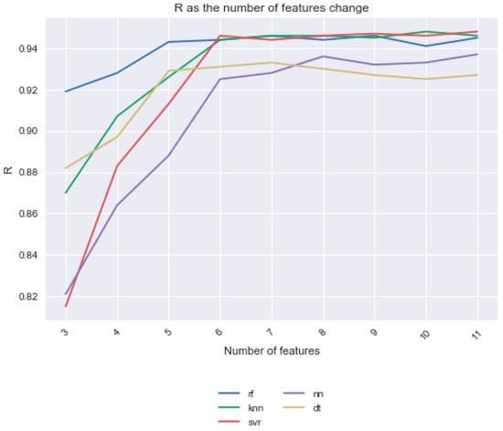
Figure 1.
Performance of models with k features and all features made available for feature selection. The average R value of the models is shown. SelectKBest feature selection was used with K values from K = 3 to K = 11. Note that the average R value for Bayesian ridge regression and linear regression were much lower than any of the other models, so they were not shown here.
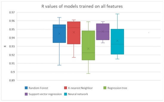
Figure 2.
The results from linear regression and Bayesian ridge regression were much lower than the other models, so their results are not shown here. The results are shown explicitly in Table 3.

Table 3.
The average scores from training the models with all possible features.
We used Weka’s Cfs method for feature selection. If all features were made available for feature selection, it found that the best features were used to both maximize the correlation between the features to the target and minimize the correlation between the features were the Julian day, total solar radiation, total rainfall, and the percent cover. The results from training the models using just these features are shown in Figure 3 and Table 4. The random forest method had achieved the highest R with a R of 0.933. The correlations between the features and target are shown in Figure 4.
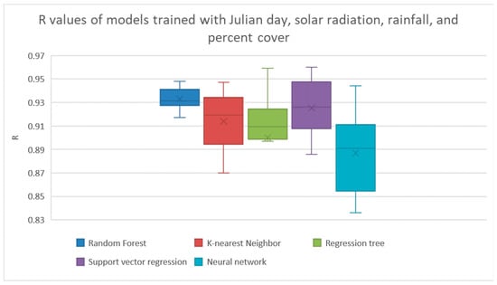
Figure 3.
Results from Cfs feature selection with all features. The results from linear regression and Bayesian ridge regression were much lower than the other models, so their results are not shown here. The results are shown explicitly in Table 4.

Table 4.
Results from Cfs feature selection with all features. These average scores are from using the features Julian day, total solar radiation, total rainfall, and percent cover.
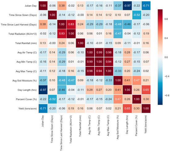
Figure 4.
Correlation heat map between features. A heat map showing the value of the correlation coefficient between each possible pair of features. We see higher correlations, positive and negative, between yield and Julian day, time since sown, radiation, rainfall, day length, and others.
However, because it may not be easy to get an accurate value of percent cover, we did another experiment with Weka’s Cfs method for feature selection. In this experiment, we made all the features available for feature selection except for percent cover. It found that the best set of features to use in this case were the Julian day, total solar radiation, total rainfall, and the number of days since the sown date. The results of evaluating the models trained on just these features are shown in Figure 5 and Table 5. The k-nearest neighbor and random forest methods both achieved the best average R with this set of features by obtaining an average R of 0.952.
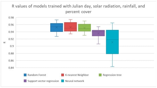
Figure 5.
Results from Cfs feature selection with no percent cover. The results from linear regression and Bayesian ridge regression were too low to show. The results are shown explicitly in Table 5.

Table 5.
Results from Cfs feature selection with no percent cover. The average scores from using the features Julian day, number of days since the sown date, total solar radiation, and total rainfall.
To compare the results obtained from using the two sets of features found by Cfs, an unpaired two-tailed t test was performed between the R values of the models trained with the features chosen by the Cfs operator (Table 6). The random forest, k-nearest neighbor, and regression tree methods performed significantly better using the feature set that excluded percent cover from being available for selection. The other methods did not vary significantly across the two sets of results. Because excluding percent cover led to results that were significantly better or the same when compared to not excluding percent cover, only the results found by Cfs without percent cover will be considered for the rest of this work.

Table 6.
p-values between the R2 values of the models trained by the two CfsSubsetEval feature sets. The results were found by doing unpaired two-tailed t tests. The first feature set contained the Julian day, total solar radiation, total rainfall, and percent cover. The second feature set contained the Julian day, the number of days since the sown date, total solar radiation, and the total rainfall. Significant results are shown in bold.
The ReliefF operator found that the best features were the number of days between the crop’s sown date and harvest date, the cumulative amount of rainfall the crop got since the previous harvest, and the average minimum daily temperature since the previous harvest. The results from training the machine learning models with these features are shown in Figure 6 and Table 7. In this case, k-nearest neighbors achieved the highest average of R with a value of 0.953.
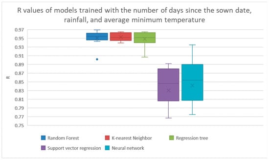
Figure 6.
Results from ReliefF feature selection. The results from linear regression and Bayesian ridge regression were much lower than the other models, so their results are not shown here. The results are shown explicitly in Table 7.

Table 7.
Results from ReliefF feature selection. The average scores from using the features number of days since the sown date, total rainfall, and the average minimum temperature since the previous harvest.
The wrapper operator reported that the best features were number of days between the crop’s sown date and harvest date, the cumulative amount of rainfall since the previous harvest, the day length at the time of the harvest, and the Julian day of the harvest. The results of the machine learning models trained on these features is shown in Figure 7 and Table 8. The best R value of these methods was also k-nearest neighbors getting an average R of 0.952.
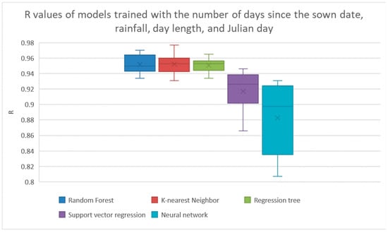
Figure 7.
Results from Wrapper feature selection operator. The results from linear regression and Bayesian ridge regression were much lower than the other models, so their results are not shown here. The results are shown explicitly in Table 8.

Table 8.
Results from Wrapper feature selection operator. The average scores from using the features number of days since the sown date, total rainfall, day length, and the Julian day.
Unpaired two-tail t tests were done between the R values of the methods that used all the features, the Cfs features (without percent cover), the ReliefF features, and the Wrapper features (Table 9). To show these results more clearly, Table 10 shows what feature selection operator led to the best results for each machine learning method. There was no significant difference in the results given by the feature selection operators in the same row of Table 10.

Table 9.
p-values between R2 values of different feature selection operators. Results from unpaired two-tail t tests. ‘All’ represents the results from Table 3, ‘Cfs’ represents the results which used the features from Figure 5/Table 5, ‘ReliefF’ represents the results from Figure 6/Table 7, and ‘Wrapper’ represents the results from Figure 7/Table 8. If a p-value is followed by a parenthesis, the value in the parentheses is an abbreviation of the feature selection method that resulted in the higher average R2 value. Lower p-values are better, and the lowest are bolded.

Table 10.
Best feature selection operators for each machine learning method. There is no significant difference between the results in the same cell. ‘All’ refers to all features being used, ‘Cfs’ refers to the set of features found by CfsSubsetEval, ‘ReliefF’ refers to the set of features found by ReliefFAttributeEval, and ’Wrapper’ refers to the set of features found by ‘WrapperSubsetEval’.
Finally, the classification tree can be found in Figure 8. A left split represents data with the attribute listed less than the value that is specified, and a right split represents the opposite. For example, the first node of the tree splits the data based on the Julian day, with data that has a Julian day of prior to the middle of May being sorted into the left child node and data that has a Julian day after this date being sorted into the right child node. The tree had 12 leaf nodes, as that was found to be the number of leaf nodes that gives the best accuracy when trees with 2–15 leaf nodes were tested. The accuracy for this final tree was found to be 85.6%, the mean absolute error was found to be 0.144 tons, and the R2 value was found to be 0.752.
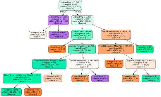
Figure 8.
The classification decision tree that sorts data into bins.
5. Discussion
Overall, this work demonstrated that we could improve on previous research to predict crop yields by applying a feature selection to our ML models. Our main improvements was a higher accuracy than the previous work, which we achieved by using a simpler dataset with fewer features, reporting our results using more intuitive and transferable metrics, and extending recent success with feature selection to the alfalfa crop.
The Cfs operator was the best overall feature selection method because it led to the best results for each method. None of the other feature selection operators led to the best results for each method. The feature set that the Cfs operator found consisted of the Julian day, the number of days between the sown and harvest date, the cumulative solar radiation since the previous harvest, and the cumulative rainfall since the last harvest.
There was no significant difference in any of the random forest results, no matter the feature selection method. The same was true for k-nearest neighbors. Even though using all features did not result in a significant difference from using a feature selection operator, it would still be beneficial to use a feature selection operator. Doing so would lower computational time and could simplify the models. The same can be said for support vector regression and the neural network, which got the best results from using either all the features or Cfs. For the regression tree, using any of the three feature selection methods resulted in better results than if all the features were used. In this case, even though fewer features were used, the results still improved. This may be because different features can embed the same information. For example, the Julian day of the harvest and the day length features both referred to seasonal information; therefore, they would have a high correlation with each other (Figure 4). Thus, including both the Julian day of the harvest and the day length could add noise to the model. For linear regression and Bayesian ridge regression, using anything but the ReliefF operator led to the best results. This is probably because forming a linear prediction function with only three features is not appropriate for this domain.
This work may be helpful because it describes a framework that can be applied to other machine learning problems in predicting crop and biomass yield. This work also shows what features are most important for predicting alfalfa yield in the southeast United States from Spring to the end of Fall. The best results came from training the models with the Julian day, the amount of solar radiation and rainfall since the previous harvest, and the number of days since the crop was sown. This is useful because gathering data is resource intensive and knowing the best features can help make data collecting more efficient. These four features are also relatively easy to obtain. The Julian day and amount of time since the crop was sown are trivial to retrieve, and the amount of solar radiation and rainfall can be obtained from weather data sources.
Moreover, besides possibly improving the results of the models, feature selection can provide insight into the problem domain [16]. By understanding what features are most important for predicting yield, one may gain insight into what factors most impact a crop’s yield. The cumulative rainfall since the previous harvest and the number of days between the harvest date and sown date were chosen by all the feature selection methods, so this is evidence that they may be the most important features for this problem. Similarly, the Julian day was chosen by two out of three feature selection methods, so this is evidence that it is also an important feature.
This work could be extended by providing this framework to alfalfa crops grown in other locations besides Georgia and Kentucky. It could also be improved by incorporating more data from other locations in the Southeast United States. This work may also be extended to use with transfer learning and domain adaptation techniques.
Supplementary Materials
The code used for this project can be found at https://github.com/chriswhitmire/alfalfa-yield-prediction.
Author Contributions
Conceptualization, C.D.W., A.M., and K.M.R.; data curation, C.D.W. and H.K.R.; methodology, C.D.W. and F.W.M.; project administration, A.M.; resources, A.M. and H.K.R.; software, H.K.R.; supervision, H.K.R.; validation, J.M.V.; writing—original draft, C.D.W.; writing—review and editing, J.M.V.; related work—J.M.V., H.K.R., and A.M. All authors have read and agreed to the published version of the manuscript.
Funding
This research received no external funding.
Informed Consent Statement
Not applicable.
Data Availability Statement
The University of Georgia alfalfa yield data can be found here: https://georgiaforages.caes.uga.edu/species-and-varieties/cool-season/alfalfa.html. The University of Kentucky alfalfa yield data can be found as progress reports on this page: http://dept.ca.uky.edu/agc/pub_prefix.asp?series=PR. Note that the only data that was used from the University of Kentucky was the non-roundup ready alfalfa varieties that were first harvested in the year 2013 or later. The daily weather data for Kentucky was found on the National Oceanic and Atmospheric Administration website: https://www.ncdc.noaa.gov/crn/qcdatasets.html. The daily weather data for Georgia was given to us by the Georgia Automated Environmental Monitoring Network. The day length was found from the United States Naval Observatory’s website: https://aa.usno.navy.mil/data/docs/Dur_OneYear.php.
Acknowledgments
We would like to thank Jonathan Markham and Shiva Makju for their assistance with compiling field data.
Conflicts of Interest
The authors declare no conflict of interest.
Appendix A
The grid for the hyperparameters of each model is as follows:
Decision Tree
- ‘criterion’: [‘mae’];
- ‘max_depth’: [5,10,25,50,100].
Random forest-
- ‘n_estimators’: [5,10,25,50,100];
- ‘max_depth’: [5,10,15,20];
- ‘criterion’: [“mae”].
K-nearest neighbors
- ‘n_neighbors’: [2,5,10];
- ‘weights’: [‘uniform’, ‘distance’];
- ‘leaf_size’: [5,10,30,50].
Support vector machine
- ‘kernel’: [‘linear’, ‘poly’, ‘rbf’, ‘sigmoid’];
- ‘C’: [0.1, 1.0, 5.0, 10.0];
- ‘gamma’: [“scale”, “auto”];
- ‘degree’: [2,3,4,5].
Neural Network
- ‘hidden_layer_sizes’: [(3), (5), (10), (3,3), (5,5), (10,10)];
- ‘‘solver’: [‘sgd’, ‘adam’];
- ‘learning_rate’: [‘constant’, ‘invscaling’, ‘adaptive’];
- ‘learning_rate_init’: [0.1, 0.01, 0.001].
Bayesian ridge regression
- ‘n_iter’: [100,300,500];
- ‘lambda_1’: [1.e−6, 1.e−4, 1.e−2, 1, 10].
Linear Regression- no hyperparameters
References
- United Nations. Transforming our world: The 2030 agenda for sustainable development. In Resolution Adopted by the General Assembly; United Nations: New York, NY, USA, 2015. [Google Scholar]
- Copenhagen Consensus Center. Background. Available online: https://www.copenhagenconsensus.com/post-2015-consensus/background (accessed on 29 December 2020).
- Rosegrant, M.W.; Magalhaes, E.; Valmonte-Santos, R.A.; Mason-D’Croz, D. Returns to investment in reducing postharvest food losses and increasing agricultural productivity growth. In Prioritizing Development: A Cost Benefit Analysis of the United Nations’ Sustainable Development Goals; Cambridge University Press: Cambridge, UK, 2018; p. 322. [Google Scholar]
- Lomborg, B. The Nobel Laureates’ Guide to the Smartest Targets for the World: 2016–2030; Copenhagen Consensus Center USA: Tewksbur, MA, USA, 2015. [Google Scholar]
- Dodds, F.; Bartram, J. (Eds.) The Water, Food, Energy and Climate Nexus: Challenges and an Agenda for Action; Routledge: Abingdon, UK, 2016. [Google Scholar]
- Bocca, F.F.; Rodrigues, L.H.A. The effect of tuning, feature engineering, and feature selection in data mining applied to rainfed sugarcane yield modelling. Comput. Electron. Agric 2016, 128, 67–76. [Google Scholar] [CrossRef]
- Feng, L.; Zhang, Z.; Ma, Y.; Du, Q.; Williams, P.; Drewry, J.; Luck, B. Alfalfa Yield Prediction Using UAV-Based Hyperspectral Imagery and Ensemble Learning. Remote Sens. 2020, 12, 2028. [Google Scholar] [CrossRef]
- Noland, R.L.; Wells, M.S.; A Coulter, J.; Tiede, T.; Baker, J.M.; Martinson, K.L.; Sheaffer, C.C. Estimating alfalfa yield and nutritive value using remote sensing and air temperature. Field Crop. Res. 2018, 222, 189–196. [Google Scholar] [CrossRef]
- Wang, Y.; Zhang, Z.; Feng, L.; Du, Q.; Runge, T. Combining Multi-Source Data and Machine Learning Approaches to Predict Winter Wheat Yield in the Conterminous United States. Remote Sens. 2020, 12, 1232. [Google Scholar] [CrossRef]
- Russell, S.J.; Norvig, P. Artificial Intelligence: A Modern Approach; Pearson Education Limited: London, UK, 2016. [Google Scholar]
- Rojas, R. Neural Networks-A Systematic Introduction; Springer: New York, NY, USA, 1996. [Google Scholar]
- Mitchell, T. Machine Learning; McGraw-Hill: New York, NY, USA, 1997. [Google Scholar]
- González Sánchez, A.; Frausto Solís, J.; Ojeda Bustamante, W. Predictive ability of machine learning methods for massive crop yield prediction. Span. J. Agric. Res. 2014. [Google Scholar] [CrossRef]
- Quinlan, J.R. Learning with continuous classes. In Proceedings of the 5th Australian Joint Conference on Artificial Intelligence, Hobart, Tasmania, 16–18 November 1992; Volume 92, pp. 343–348. [Google Scholar]
- Gelman, A.; Stern, H.S.; Carlin, J.B.; Dunson, D.B.; Vehtari, A.; Rubin, D.B. Bayesian Data Analysis; Chapman and Hall/CRC: Abingdon, UK, 2013. [Google Scholar]
- Dash, M.; Liu, H. Feature Selection for Classification. Intelligent Data Analysis; IOS Press: Amsterdam, The Netherlands, 1997; Volume 1, pp. 131–156. [Google Scholar]
- Hall, M.A. Correlation-Based Feature Selection for Machine Learning. Ph.D. Thesis, University of Waikato, Hamilton, New Zealand, 1999. [Google Scholar]
- Kononenko, I. Estimating Attributes: Analysis and Extensions of RELIEF. In Proceedings of the European Conference on Machine Learning, Catania, Italy, 6–8 April 1994; Springer: Berlin/Heidelberg, Germany, 1994; pp. 171–182. [Google Scholar]
- Ratner, B. The correlation coefficient: Its values range between +1/−1, or do they? J. Target. Meas. Anal. Mark. 2009, 17, 139–142. [Google Scholar] [CrossRef]
- Boote, K.J.; Jones, J.W.; Hoogenboom, G.; Pickering, N.B. The CROPGRO model for grain legumes. In Applications of Systems Approaches at the Field Level; Springer Science and Business Media LLC: Berlin/Heidelberg, Germany, 1998; pp. 99–128. [Google Scholar]
- Malik, W.; Boote, K.J.; Hoogenboom, G.; Cavero, J.; Dechmi, F. Adapting the CROPGRO Model to Simulate Alfalfa Growth and Yield. Agron. J. 2018, 110, 1777–1790. [Google Scholar] [CrossRef]
- Jing, Q.; Qian, B.; Bélanger, G.; Vanderzaag, A.; Jégo, G.; Smith, W.; Grant, B.; Shang, J.; Liu, J.; He, W.; et al. Simulating alfalfa regrowth and biomass in eastern Canada using the CSM-CROPGRO-perennial forage model. Eur. J. Agron. 2020, 113, 125971. [Google Scholar] [CrossRef]
- YangiD, P.; Zhao, Q.; Cai, X. Machine learning based estimation of land productivity in the contiguous US using biophysical predictors. Environ. Res. Lett. 2020, 15, 074013. [Google Scholar] [CrossRef]
- Leng, G.; Hall, J.W. Predicting spatial and temporal variability in crop yields: An inter-comparison of machine learning, regression and process-based models. Environ. Res. Lett. 2020, 15, 044027. [Google Scholar] [CrossRef]
- Nikoloski, S.; Murphy, P.; Kocev, D.; Džeroski, S.; Wall, D.P. Using machine learning to estimate herbage production and nutrient uptake on Irish dairy farms. J. Dairy Sci. 2019, 102, 10639–10656. [Google Scholar] [CrossRef]
- McKinney, W. Data Structures for Statistical Computing in Python. In Proceedings of the 9th Python in Science Conference, Austin, TX, USA, 28 June–3 July 2010; pp. 51–56. [Google Scholar]
- Hunter, J.D. Matplotlib: A 2D Graphics Environment. Comput. Sci. Eng. 2007, 9, 90–95. [Google Scholar] [CrossRef]
- Waskom, M.; Botvinnik, O.; Drewokane; Hobson, P.; David; Halchenko, Y.; Lee, A. Seaborn: v0. 7.1. Zenodo 2016. [Google Scholar] [CrossRef]
- Pedregosa, F.; Varoquaux, G.; Gramfort, A.; Michel, V.; Thirion, B.; Grisel, O.; Vanderplas, J. Scikit-learn: Machine learning in Python. J. Mach. Learn. Res. 2011, 12, 2825–2830. [Google Scholar]
- Oliphant, T.E. A Guide to NumPy; Trelgol Publishing: Wilmington, DE, USA, 2006; Volume 1, p. 85. [Google Scholar]
- Van Der Walt, S.; Colbert, S.C.; Varoquaux, G. The NumPy Array: A Structure for Efficient Numerical Computation. Comput. Sci. Eng. 2011, 13, 22–30. [Google Scholar] [CrossRef]
- Witten, I.H.; Frank, E.; Hall, M.A. Data Mining: Practical Machine Learning Tools and Techniques, 3rd ed.; Elsevier Morgan Kaufmann: San Francisco, CA, USA, 2011. [Google Scholar]
Publisher’s Note: MDPI stays neutral with regard to jurisdictional claims in published maps and institutional affiliations. |
© 2021 by the authors. Licensee MDPI, Basel, Switzerland. This article is an open access article distributed under the terms and conditions of the Creative Commons Attribution (CC BY) license (http://creativecommons.org/licenses/by/4.0/).