Figure 1.
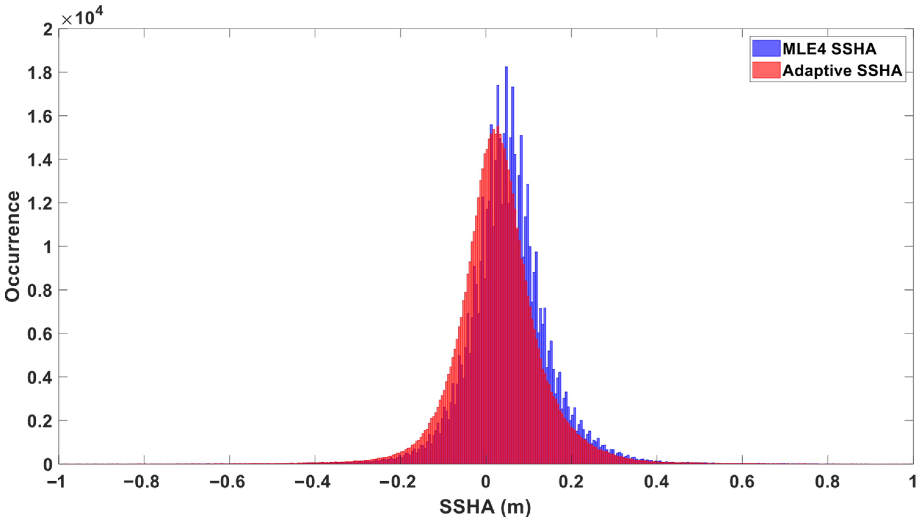
Histogram of SSHA Distribution for Cycle #399 (Blue: MLE4, Red: Adaptive; Data Unedited).
Figure 1.
Histogram of SSHA Distribution for Cycle #399 (Blue: MLE4, Red: Adaptive; Data Unedited).
Figure 2.
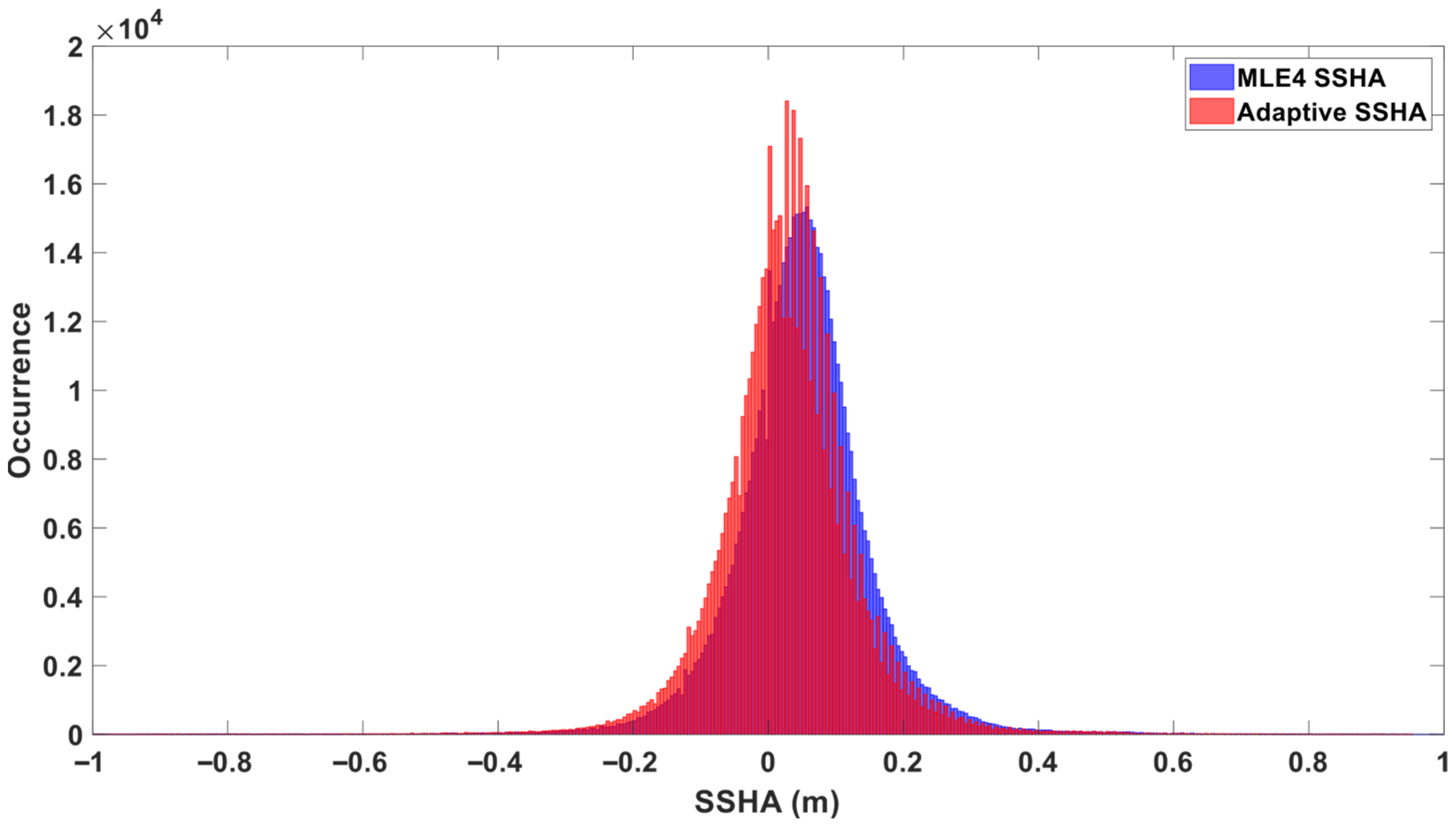
Histogram of SSHA Distribution for Cycle #501 (Blue: MLE4, Red: Adaptive; Data Unedited).
Figure 2.
Histogram of SSHA Distribution for Cycle #501 (Blue: MLE4, Red: Adaptive; Data Unedited).
Figure 3.
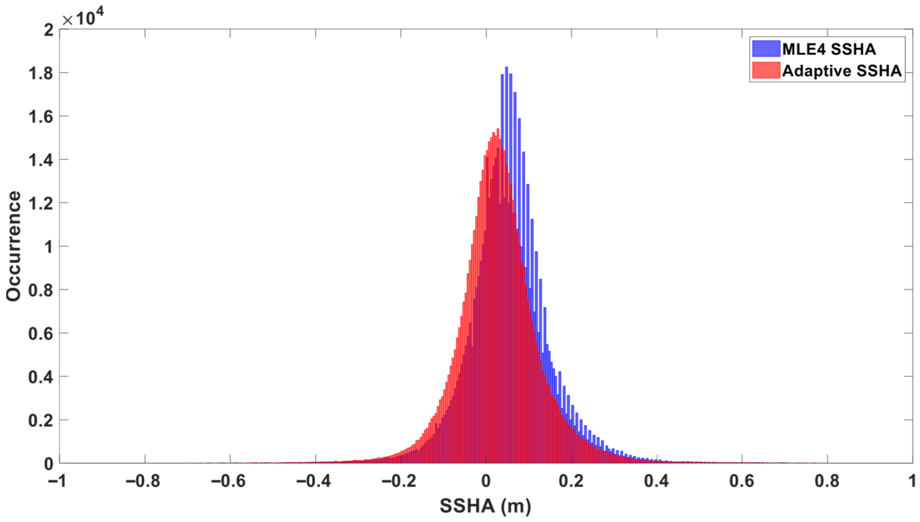
Histogram of SSHA Distribution for Cycle #399 (Blue: MLE4, Red: Adaptive; Data Edited, Open Ocean Data Retained).
Figure 3.
Histogram of SSHA Distribution for Cycle #399 (Blue: MLE4, Red: Adaptive; Data Edited, Open Ocean Data Retained).
Figure 4.
Histogram of SSHA Distribution for Cycle #501 (Blue: MLE4, Red: Adaptive; Data Edited, Open Ocean Data Retained).
Figure 4.
Histogram of SSHA Distribution for Cycle #501 (Blue: MLE4, Red: Adaptive; Data Edited, Open Ocean Data Retained).
Figure 5.
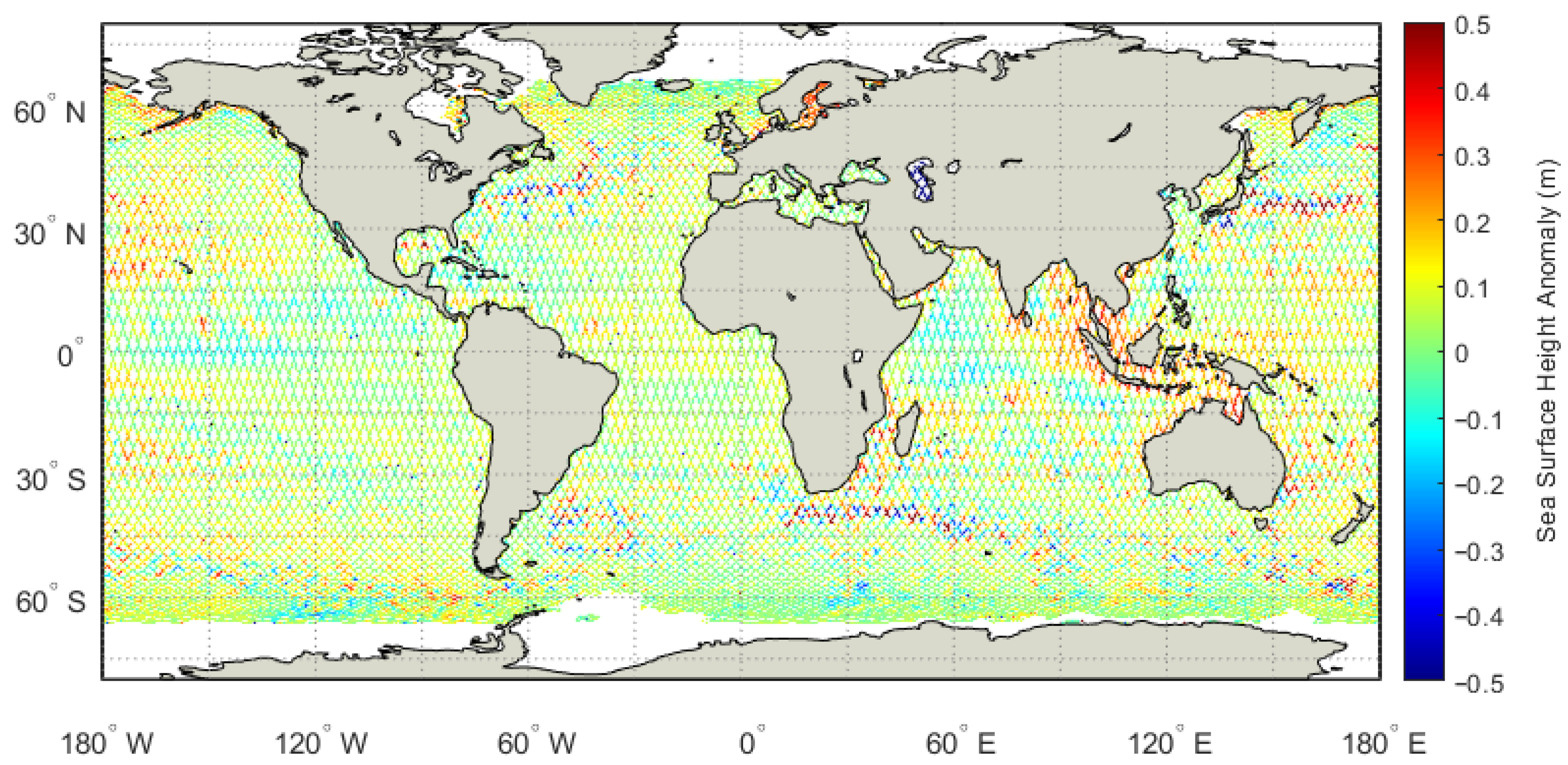
Schematic diagram of Jason-3 satellite altimeter SSHA (Cycle #399, GDR-F).
Figure 5.
Schematic diagram of Jason-3 satellite altimeter SSHA (Cycle #399, GDR-F).
Figure 6.
Schematic diagram of Jason-3 satellite altimeter SSHA (Cycle #501, GDR-G).
Figure 6.
Schematic diagram of Jason-3 satellite altimeter SSHA (Cycle #501, GDR-G).
Figure 7.
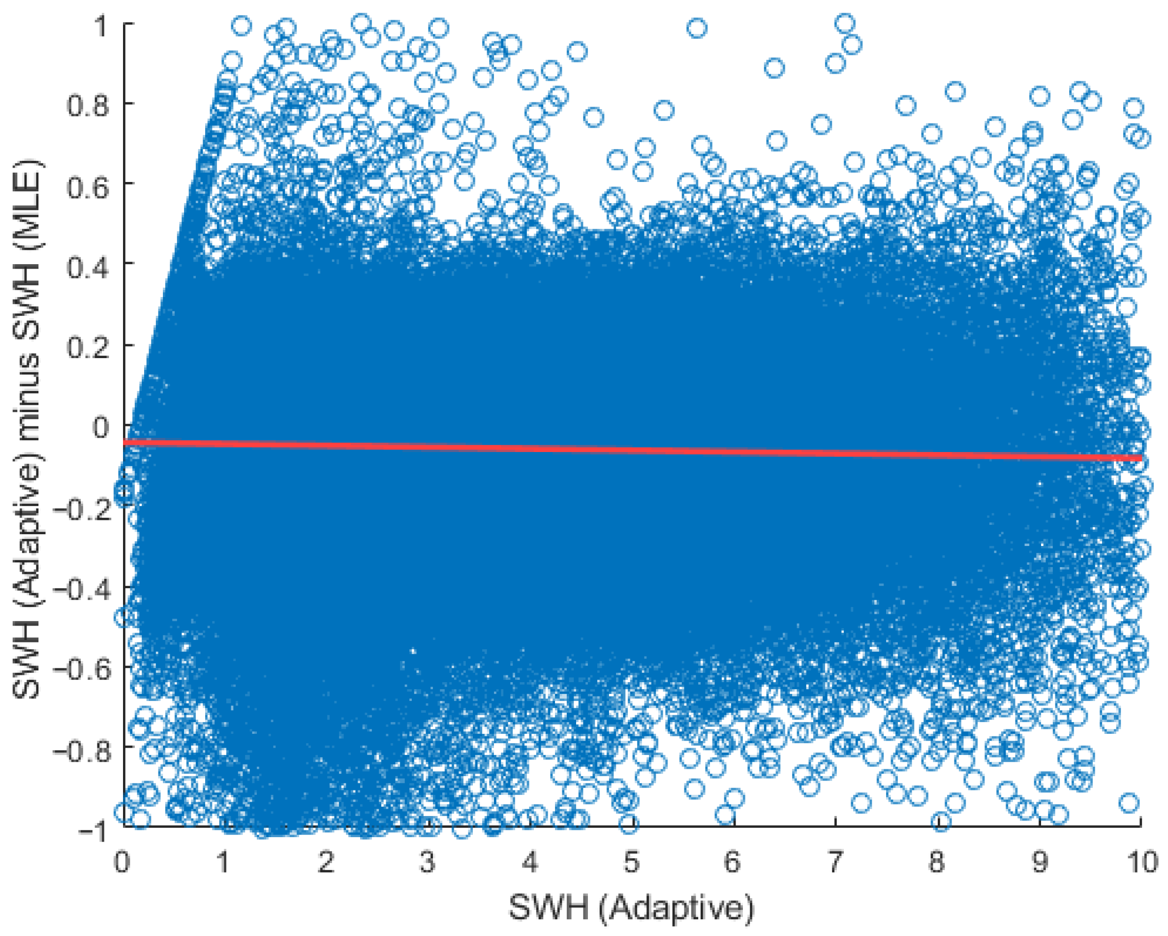
Linear regression analysis between the Adaptive SWH and the SWH difference (Adaptive SWH minus MLE4 SWH) for Cycle #501. The blue circles were the pairs of the Adaptive SWH and the SWH difference. The thick red line illustrated the trend (Slope = −0.00396, Offset = −0.043).
Figure 7.
Linear regression analysis between the Adaptive SWH and the SWH difference (Adaptive SWH minus MLE4 SWH) for Cycle #501. The blue circles were the pairs of the Adaptive SWH and the SWH difference. The thick red line illustrated the trend (Slope = −0.00396, Offset = −0.043).
Figure 8.
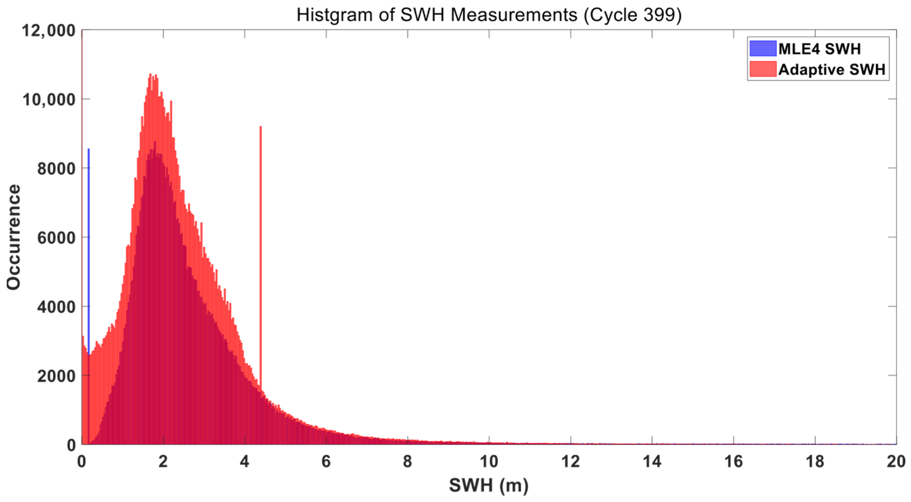
Histogram of SWH Distribution for Cycle #399 (Blue: MLE4, Red: Adaptive Method; Data Unedited).
Figure 8.
Histogram of SWH Distribution for Cycle #399 (Blue: MLE4, Red: Adaptive Method; Data Unedited).
Figure 9.
Histogram of SWH Distribution for Cycle #501 (Blue: MLE4, Red: Adaptive Method; Data Unedited).
Figure 9.
Histogram of SWH Distribution for Cycle #501 (Blue: MLE4, Red: Adaptive Method; Data Unedited).
Figure 10.
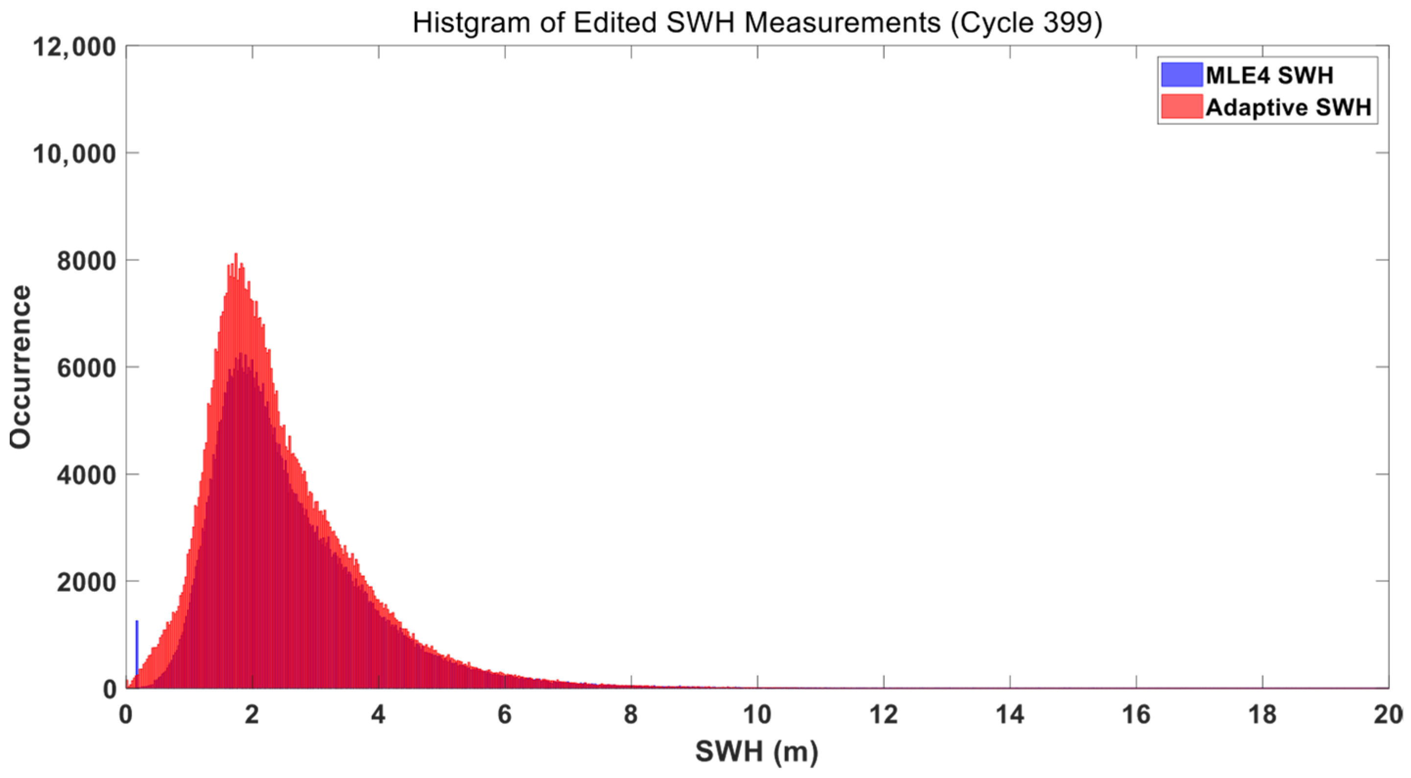
Histogram of SWH Distribution for Cycle #399 (Blue: MLE4, Red: Adaptive Method; Data Edited, Open Ocean Data Retained).
Figure 10.
Histogram of SWH Distribution for Cycle #399 (Blue: MLE4, Red: Adaptive Method; Data Edited, Open Ocean Data Retained).
Figure 11.
Histogram of SWH Distribution for Cycle #501 (Blue: MLE4, Red: Adaptive Method; Data Edited, Open Ocean Data Retained).
Figure 11.
Histogram of SWH Distribution for Cycle #501 (Blue: MLE4, Red: Adaptive Method; Data Edited, Open Ocean Data Retained).
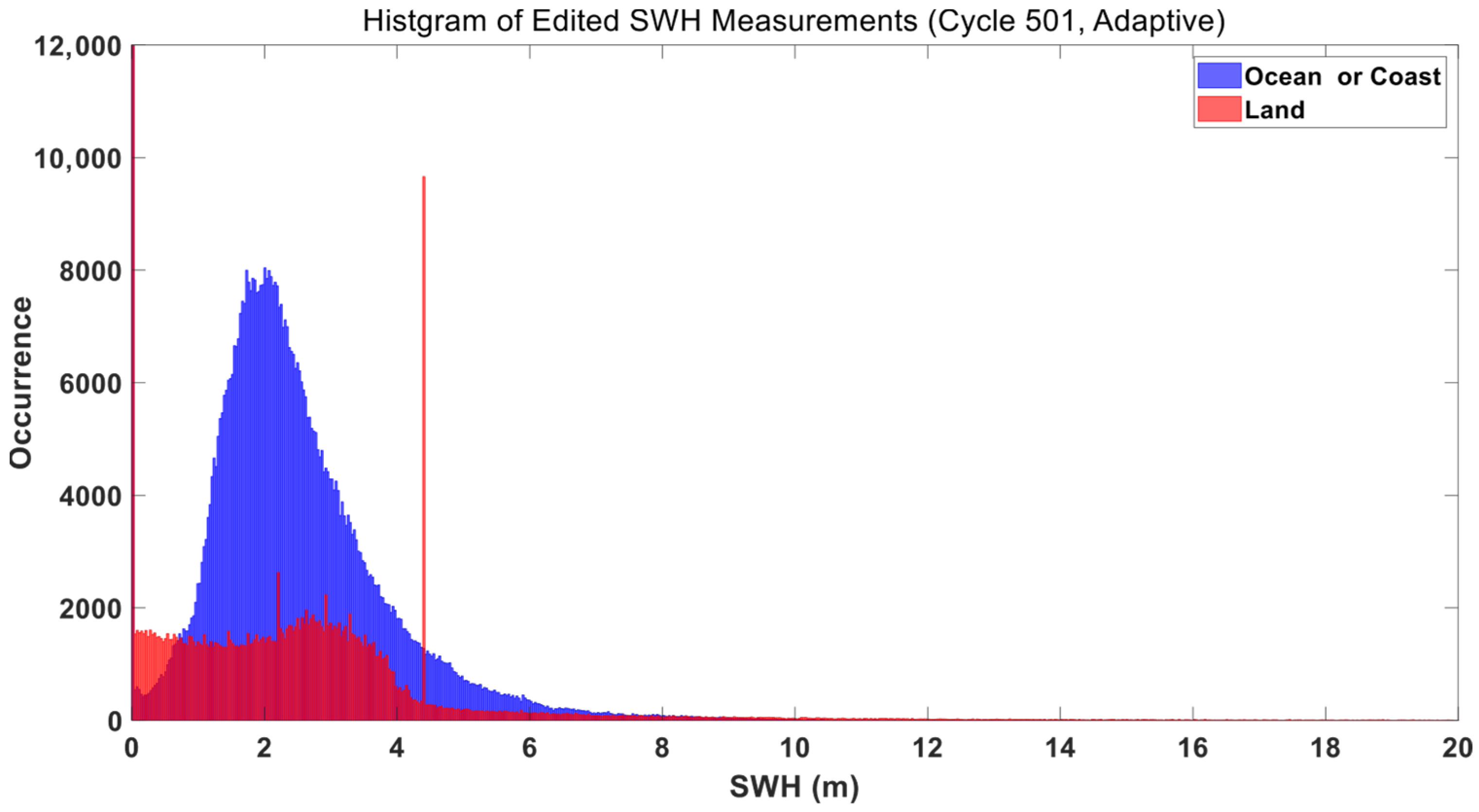
Figure 12.
Histogram of SWH Distribution for Cycle #501 (Blue: Ocean or Coast, Red: Land).
Figure 12.
Histogram of SWH Distribution for Cycle #501 (Blue: Ocean or Coast, Red: Land).
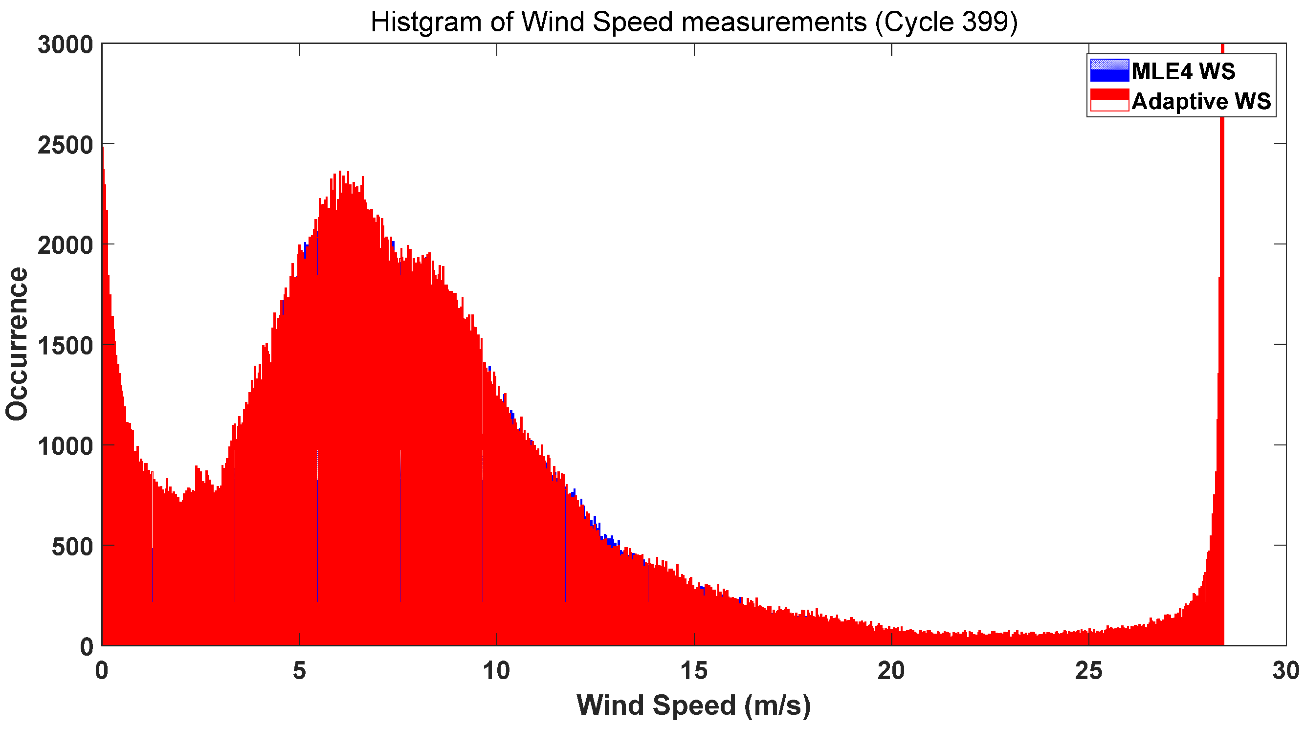
Figure 13.
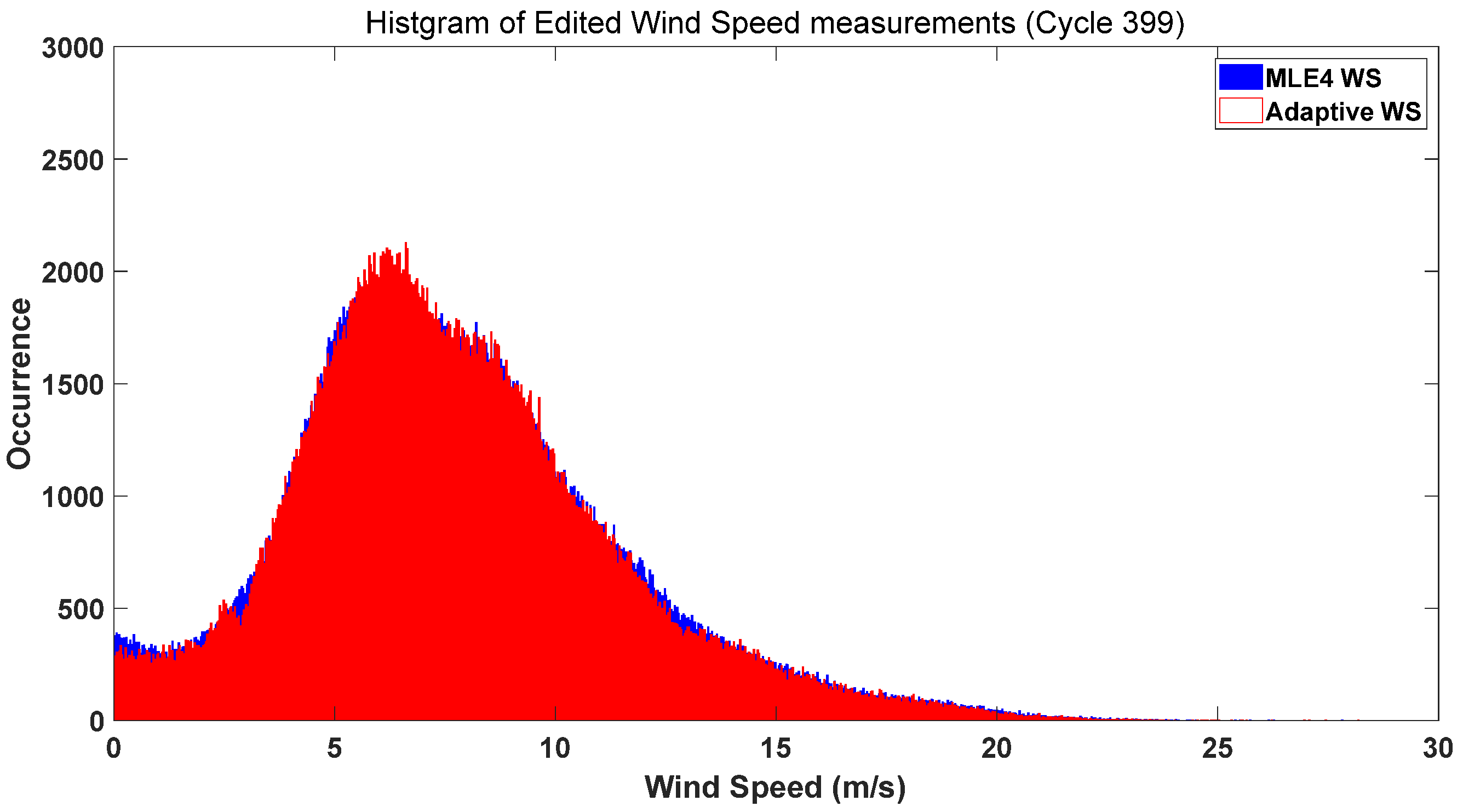
Histogram of WS Distribution for Cycle #399 (Blue: MLE4, Red: Adaptive Method; Data Unedited).
Figure 13.
Histogram of WS Distribution for Cycle #399 (Blue: MLE4, Red: Adaptive Method; Data Unedited).
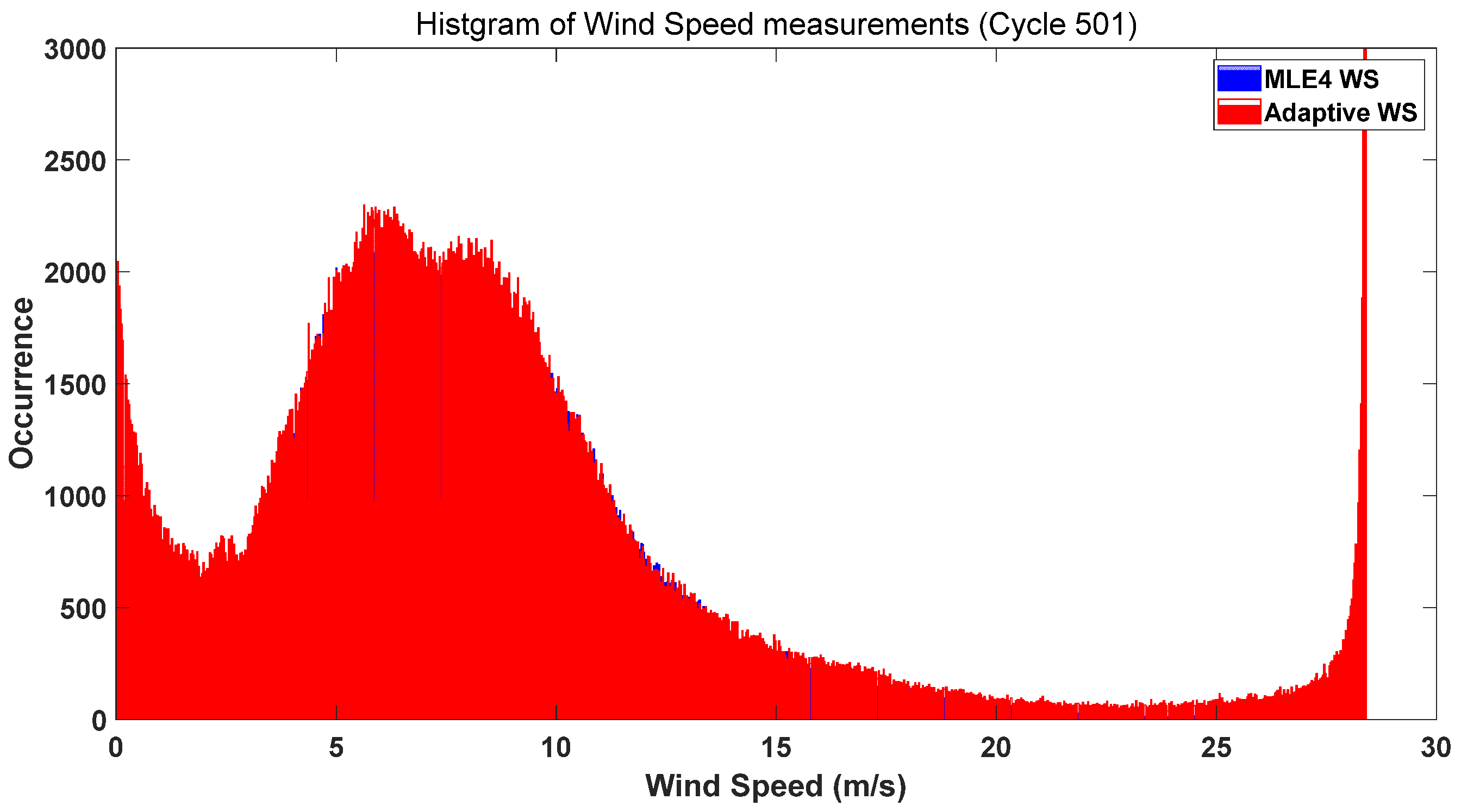
Figure 14.
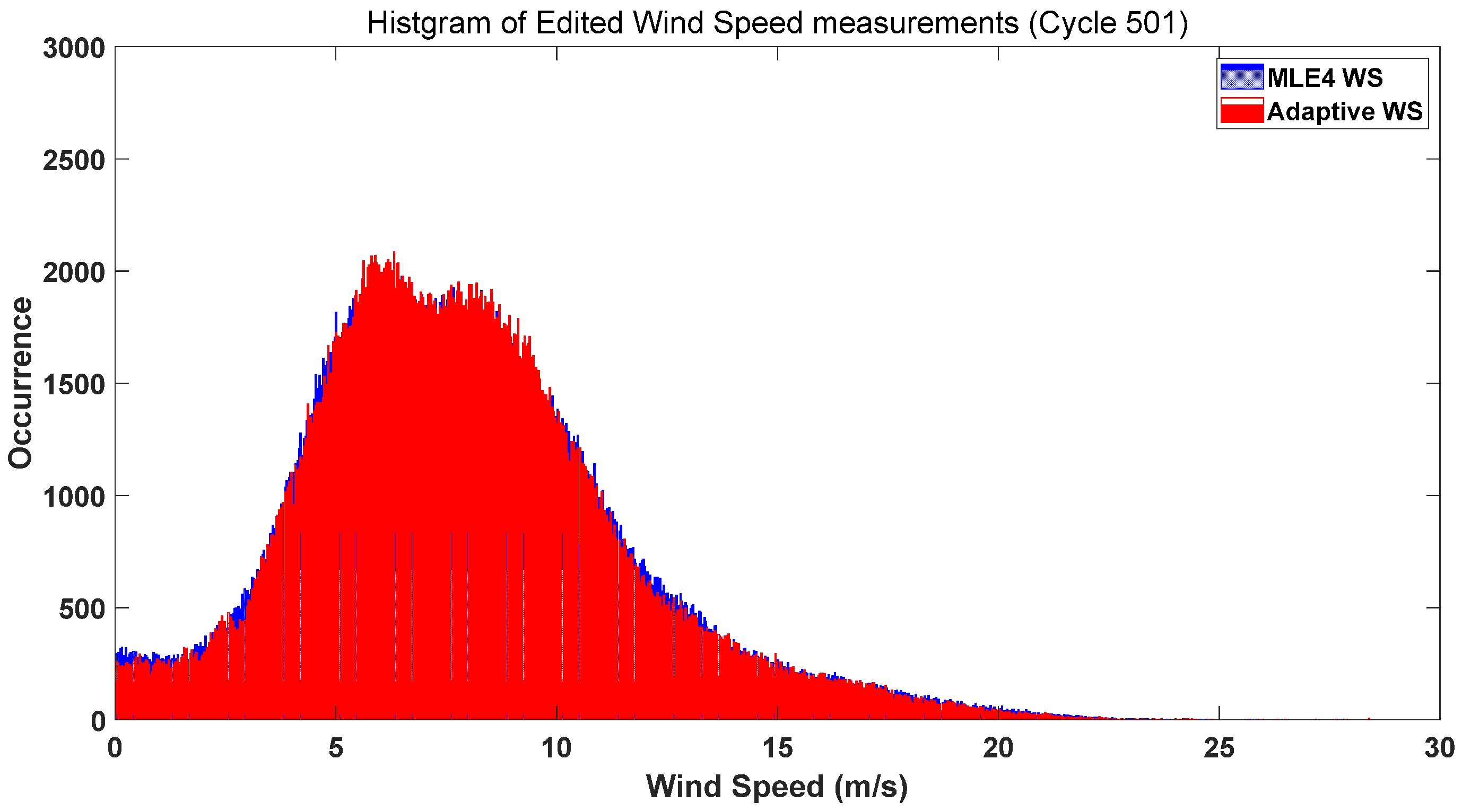
Histogram of WS Distribution for Cycle #501 (Blue: MLE4, Red: Adaptive Method; Data Unedited).
Figure 14.
Histogram of WS Distribution for Cycle #501 (Blue: MLE4, Red: Adaptive Method; Data Unedited).
Figure 15.
Histogram of WS Distribution for Cycle #399 (Blue: MLE4, Red: Adaptive Method; Data Edited, Open Ocean Data Retained).
Figure 15.
Histogram of WS Distribution for Cycle #399 (Blue: MLE4, Red: Adaptive Method; Data Edited, Open Ocean Data Retained).
Figure 16.
Histogram of WS Distribution for Cycle #501 (Blue: MLE4, Red: Adaptive Method; Data Edited, Open Ocean Data Retained).
Figure 16.
Histogram of WS Distribution for Cycle #501 (Blue: MLE4, Red: Adaptive Method; Data Edited, Open Ocean Data Retained).
Figure 17.
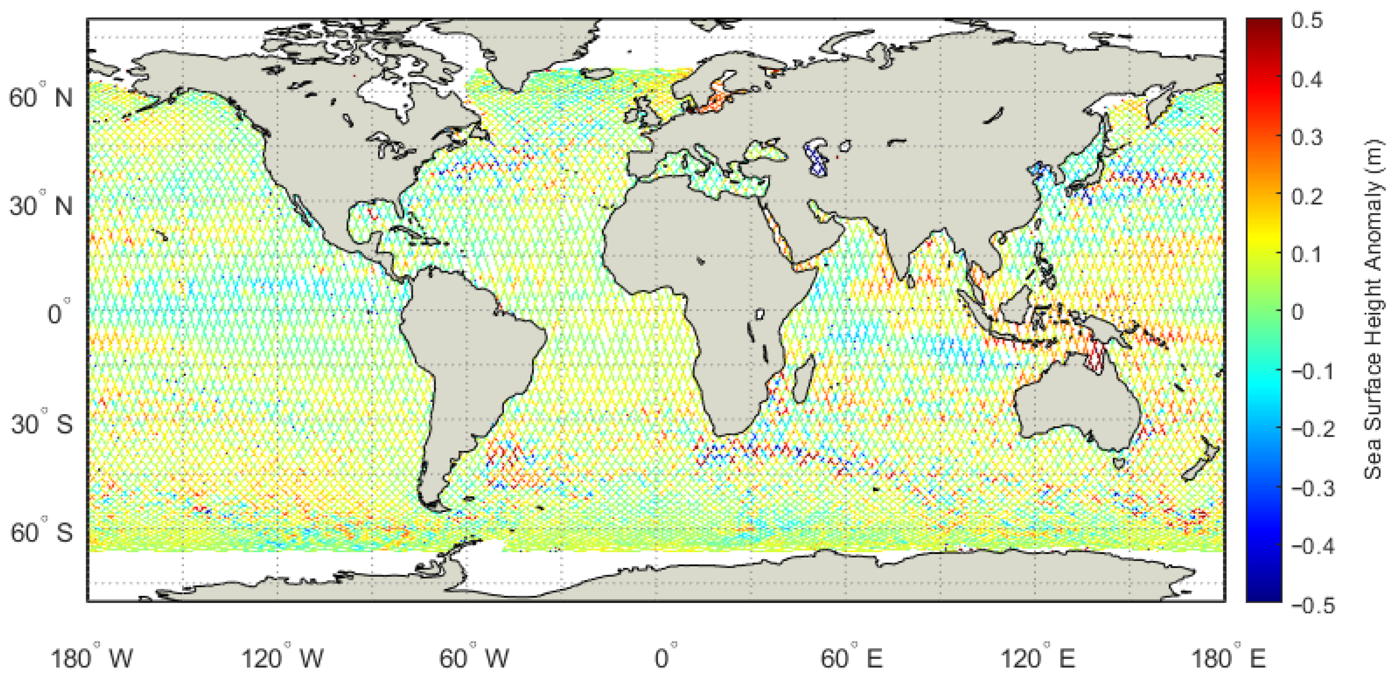
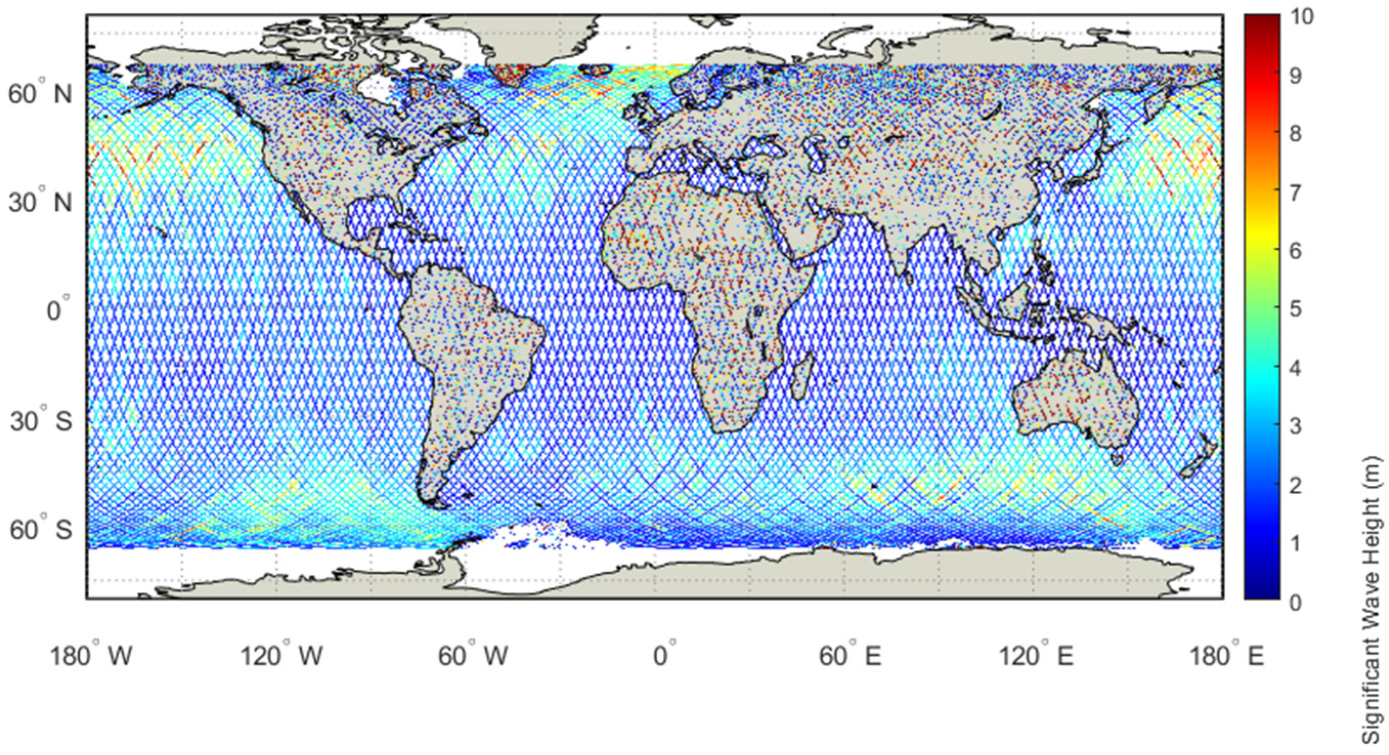
Geographical distribution map of SWH from Jason-3 satellite altimeter (Cycle #399, GDR-F).
Figure 17.
Geographical distribution map of SWH from Jason-3 satellite altimeter (Cycle #399, GDR-F).
Figure 18.
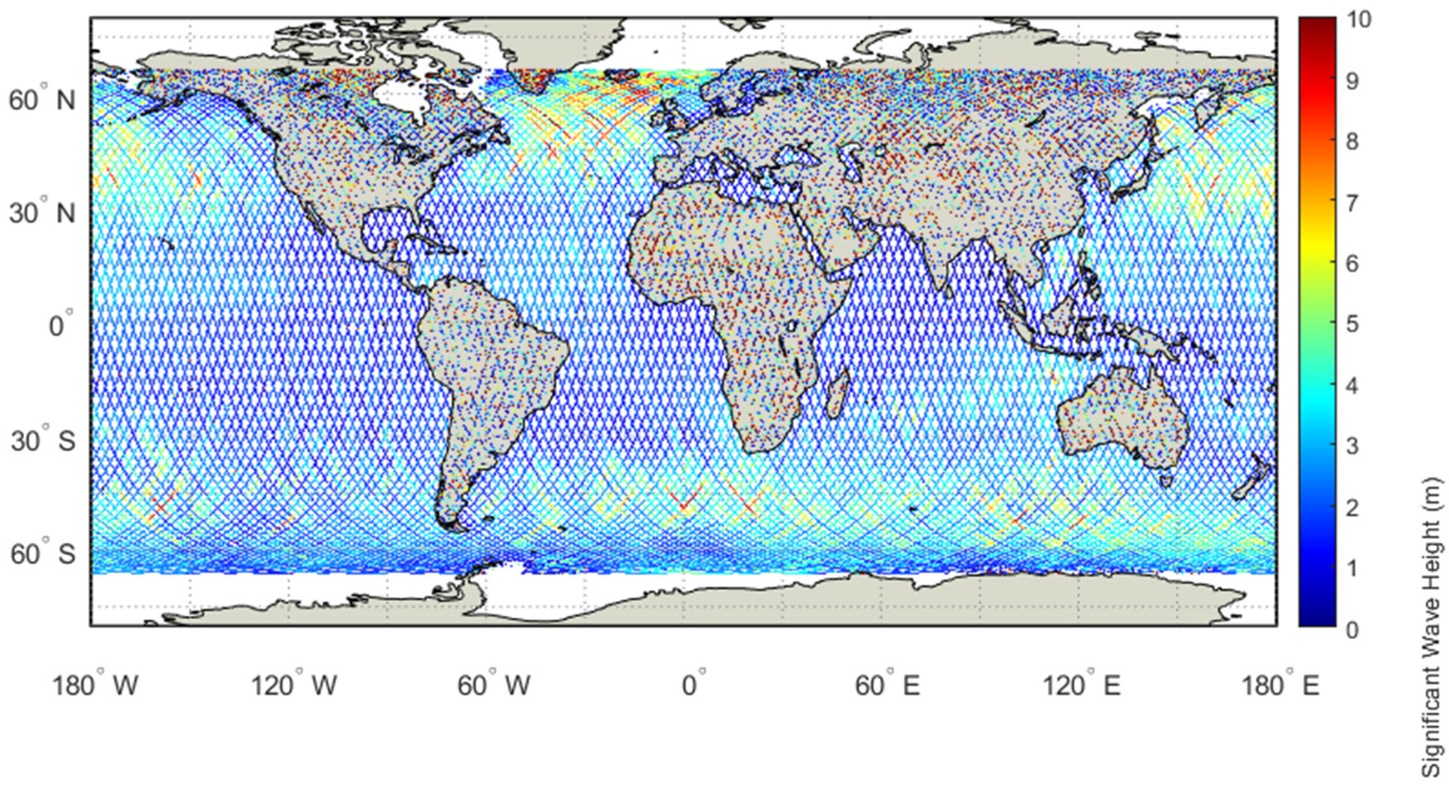
Geographical distribution map of SWH from Jason-3 satellite altimeter (Cycle #501, GDR-G).
Figure 18.
Geographical distribution map of SWH from Jason-3 satellite altimeter (Cycle #501, GDR-G).
Figure 19.
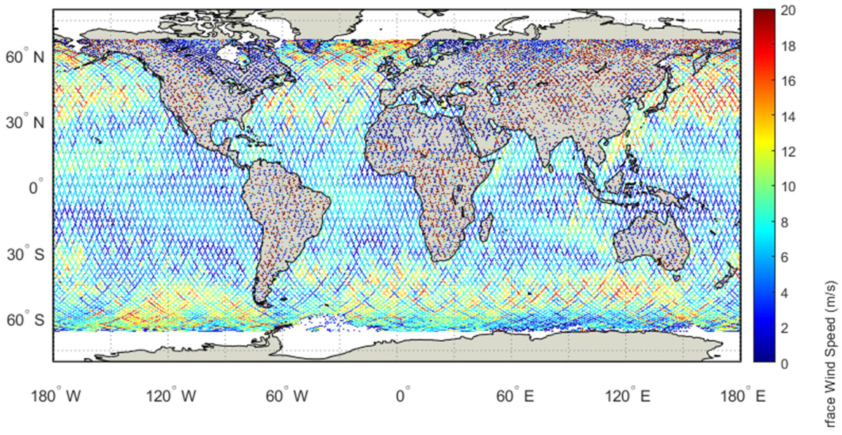
Geographical distribution map of WS from Jason-3 satellite altimeter (Cycle #399, GDR-F).
Figure 19.
Geographical distribution map of WS from Jason-3 satellite altimeter (Cycle #399, GDR-F).
Figure 20.
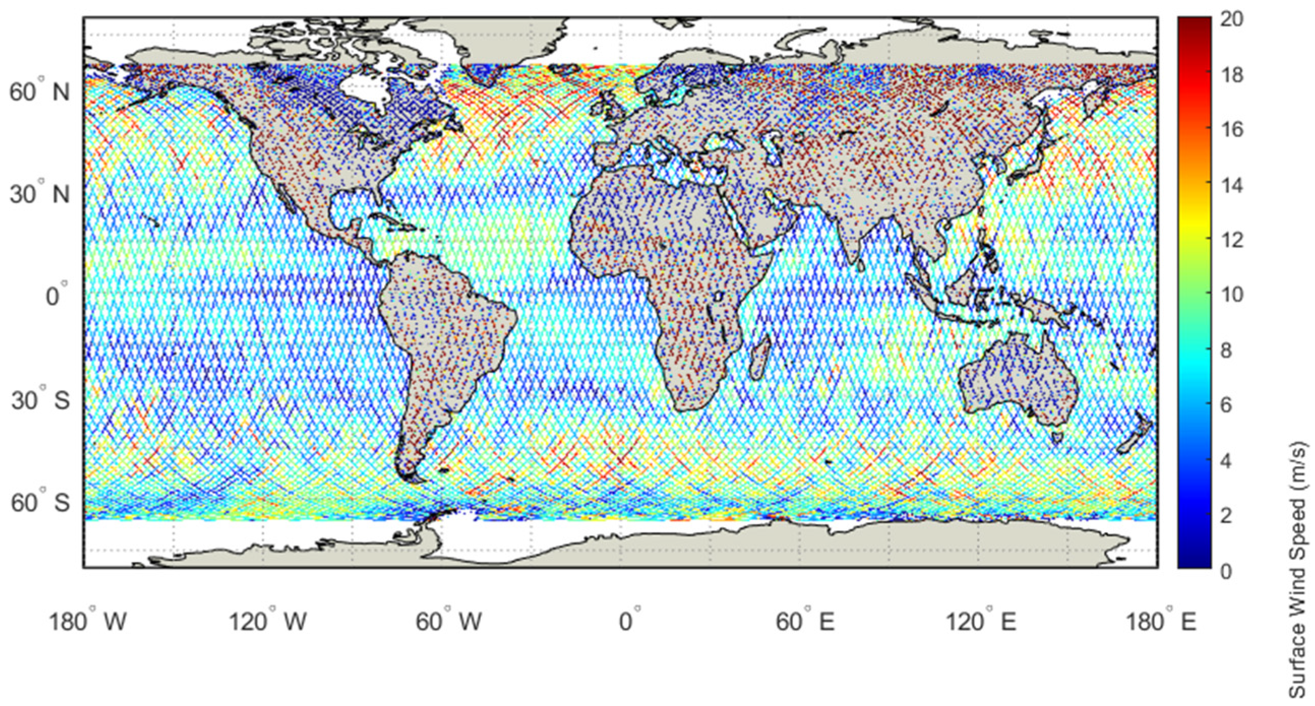
Geographical distribution map of WS from Jason-3 satellite altimeter (Cycle #501, GDR-G).
Figure 20.
Geographical distribution map of WS from Jason-3 satellite altimeter (Cycle #501, GDR-G).
Figure 21.
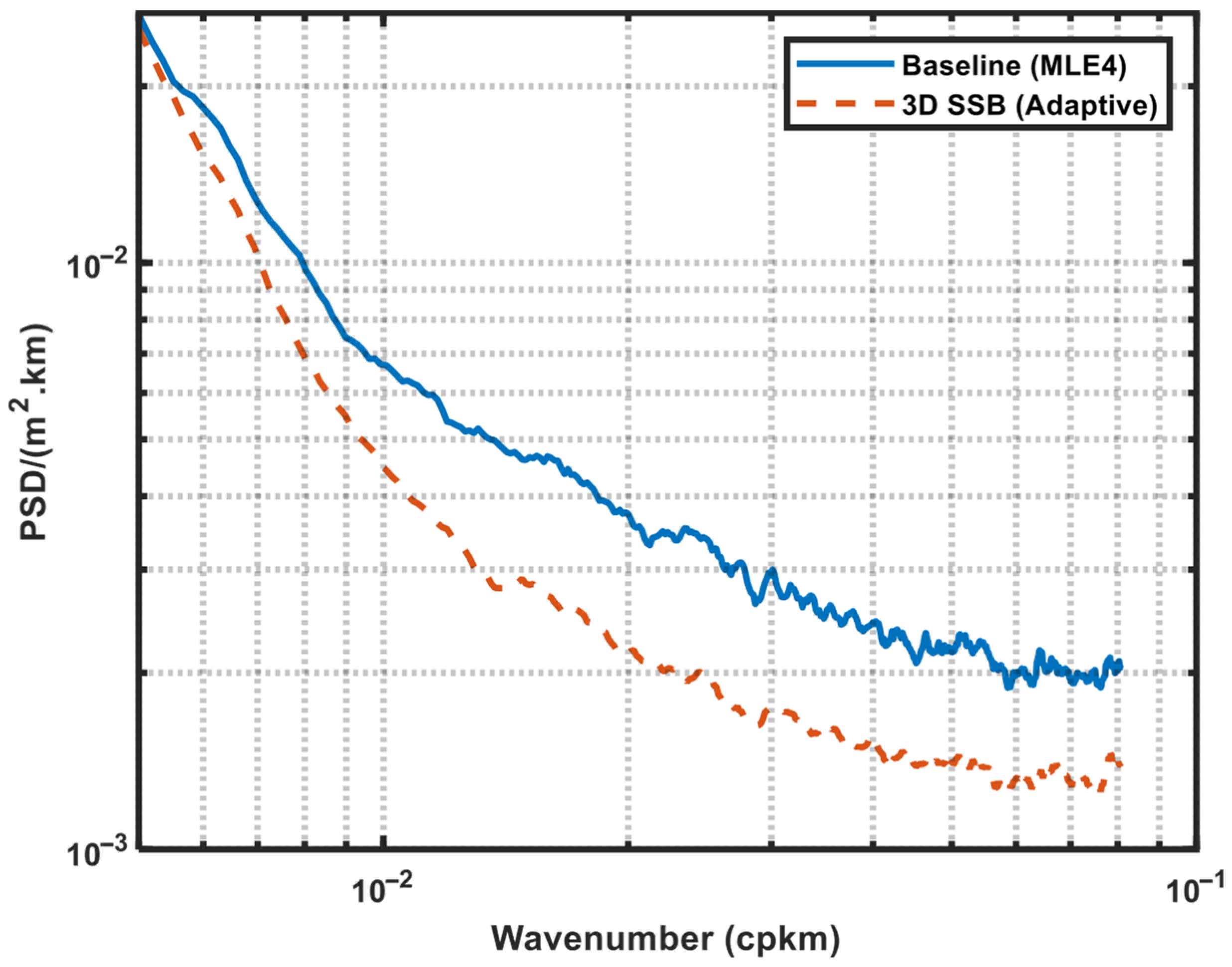
SSHA spectrums from Jason-3 satellite altimeter (Cycle #394–#399, GDR-F). The blue curve was for the Baseline (MLE4) SSHA, and the red curve was for the most precise 3D SSB (Adaptive) SSHA.
Figure 21.
SSHA spectrums from Jason-3 satellite altimeter (Cycle #394–#399, GDR-F). The blue curve was for the Baseline (MLE4) SSHA, and the red curve was for the most precise 3D SSB (Adaptive) SSHA.
Figure 22.
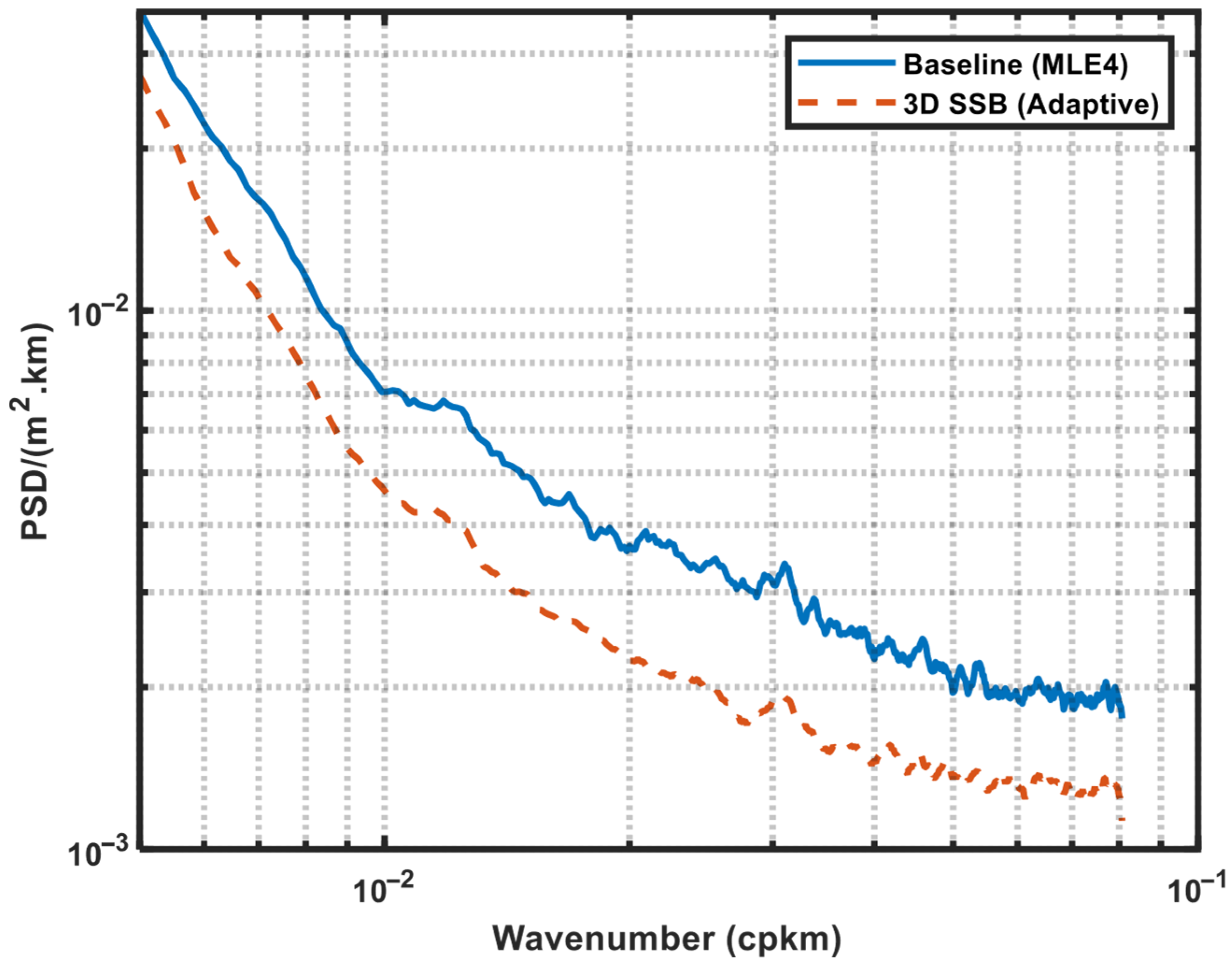
SSHA spectrums from Jason-3 satellite altimeter (Cycle #501–#506, GDR-G). The blue curve was for the Baseline (MLE4) SSHA, and the red curve was for the most precise 3D SSB (Adaptive) SSHA.
Figure 22.
SSHA spectrums from Jason-3 satellite altimeter (Cycle #501–#506, GDR-G). The blue curve was for the Baseline (MLE4) SSHA, and the red curve was for the most precise 3D SSB (Adaptive) SSHA.
Table 1.
Evolution of the Models from Jason-3 GDR-F to Jason-3 GDR-G.
Table 1.
Evolution of the Models from Jason-3 GDR-F to Jason-3 GDR-G.
| Model | GDR-F | GDR-G |
|---|
| Orbit model | MOE/POE-F | MOE/POE-G |
| FES Ocean and load tide model | FES2014B | FES2022B |
| MSS models 1 | CNES_CLS-2015 + DTU18 | Hybrid 2023 + DTU21 |
| MDT model 1 | CNES_CLS_MDT-2018 | CNES_CLS_MDT-2022 |
Table 2.
Date, Mission, Cycle number and the corresponding processing standards of the data used in this study.
Table 2.
Date, Mission, Cycle number and the corresponding processing standards of the data used in this study.
| Date | Mission | Cycle Number | Processing Standards |
|---|
| 6 November 2024 to 2 January 2025 | Jason-3 | #394–#399 | GDR-F |
| Sentinel-6A | #156~#161 | GDR-F (LR) |
| 1 February 2025–1 May 2025 | Jason-3 | #501~#509 | GDR-F |
| Sentinel-6A | #156~#159 | GDR-F (LR) |
| Sentinel-6A | #160~#164 | GDR-G (LR) |
Table 3.
Candidate solutions of several correction items.
Table 3.
Candidate solutions of several correction items.
| Correction Item | Baseline Solution | Secondary Solution |
|---|
| Wet tropospheric delay | Microwave radiometer | ECMWF model |
| Ionospheric delay | Dual-frequency altimetry | GIM model |
| Sea state bias | 2D model | 3D model |
| Ocean tide 1 | FES model | GOT model |
| MSS | CNES_CLS (F)/Hybrid (G) | DTU model |
Table 4.
SSHA mean values and relative biases to the baseline product under the eight approaches (Unit: centimeters; GDR-F SSHAs were averaged from Cycles #394–#399, and GDR-G SSHAs were averaging from Cycles #501–#506).
Table 4.
SSHA mean values and relative biases to the baseline product under the eight approaches (Unit: centimeters; GDR-F SSHAs were averaged from Cycles #394–#399, and GDR-G SSHAs were averaging from Cycles #501–#506).
| Approach | GDR-F SSHA Average | ΔSSHA | GDR-G SSHA Average | ΔSSHA |
|---|
| Baseline (MLE4) | 5.40 | 0 | 5.03 | 0 |
| 3D SSB (MLE4) | 7.05 | 1.65 | 6.60 | 1.57 |
| Model wet path (MLE4) | 5.64 | 0.24 | 5.15 | 0.12 |
| GIM ionospheric (MLE4) | 6.89 | 1.48 | 6.65 | 1.62 |
| GOT tide (MLE4) | 5.43 | 0.03 | 5.06 | 0.03 |
| DTU MSS (MLE4) | 5.98 | 0.58 | 5.12 | 0.08 |
| Baseline (Adaptive) | 2.94 | −2.46 | 2.56 | −2.48 |
| 3D SSB (Adaptive) | 4.46 | −0.94 | 4.02 | −1.01 |
Table 5.
SSHA standard deviations under different processing approaches (Unit: centimeters, GDR-F, cycle #394–#399, 41-point Lanczos kernel).
Table 5.
SSHA standard deviations under different processing approaches (Unit: centimeters, GDR-F, cycle #394–#399, 41-point Lanczos kernel).
| Approach | Cycle #394 | Cycle #395 | Cycle #396 | Cycle #397 | Cycle #398 | Cycle #399 | Average |
|---|
| Baseline (MLE4) | 4.16 | 4.15 | 4.05 | 4.02 | 4.09 | 4.06 | 4.09 |
| 3D SSB (MLE4) | 4.00 | 4.01 | 3.90 | 3.89 | 3.95 | 3.95 | 3.95 |
| Model wet tropospheric (MLE4) | 4.18 | 4.17 | 4.06 | 4.04 | 4.10 | 4.08 | 4.11 |
| GIM ionospheric (MLE4) | 4.19 | 4.18 | 4.08 | 4.05 | 4.10 | 4.08 | 4.11 |
| GOT tide (MLE4) | 4.17 | 4.15 | 4.05 | 4.02 | 4.09 | 4.07 | 4.09 |
| DTU MSS (MLE4) | 4.22 | 4.21 | 4.11 | 4.08 | 4.14 | 4.13 | 4.15 |
| Baseline (Adaptive) | 3.86 | 3.96 | 3.73 | 3.76 | 3.82 | 3.76 | 3.82 |
| 3D SSB (Adaptive) | 3.74 | 3.86 | 3.63 | 3.65 | 3.71 | 3.65 | 3.71 |
Table 6.
SSHA standard deviations under different processing approaches (Unit: centimeters, GDR-G, cycle #501–#506, 41-point Lanczos kernel).
Table 6.
SSHA standard deviations under different processing approaches (Unit: centimeters, GDR-G, cycle #501–#506, 41-point Lanczos kernel).
| Approach | Cycle #501 | Cycle #502 | Cycle #503 | Cycle #504 | Cycle #505 | Cycle #506 | Average |
|---|
| Baseline (MLE4) | 3.97 | 4.08 | 4.06 | 4.14 | 4.06 | 3.98 | 4.05 |
| 3D SSB (MLE4) | 3.84 | 3.95 | 3.93 | 3.99 | 3.91 | 3.88 | 3.92 |
| Model wet path (MLE4) | 3.98 | 4.10 | 4.07 | 4.15 | 4.08 | 4.00 | 4.06 |
| GIM ionospheric (MLE4) | 3.99 | 4.10 | 4.08 | 4.16 | 4.08 | 4.01 | 4.07 |
| GOT tide (MLE4) | 3.98 | 4.08 | 4.07 | 4.14 | 4.06 | 3.99 | 4.05 |
| DTU MSS (MLE4) | 3.99 | 4.10 | 4.07 | 4.16 | 4.09 | 4.01 | 4.07 |
| Baseline (Adaptive) | 3.70 | 3.81 | 3.76 | 3.80 | 3.78 | 3.70 | 3.76 |
| 3D SSB (Adaptive) | 3.59 | 3.69 | 3.64 | 3.68 | 3.66 | 3.60 | 3.64 |
Table 7.
SSHA improvement or degradation over the MEL4 baseline SSHA (Unit: centimeters, Detrend method, 41-point Lanczos kernel).
Table 7.
SSHA improvement or degradation over the MEL4 baseline SSHA (Unit: centimeters, Detrend method, 41-point Lanczos kernel).
| Approach | GDR-F | GDR-G | Improvement of GDR-G Over GDR-F Mean Detrend SSHA Noise Level |
|---|
| Mean Detrend SSHA Noise Level | Improvement or Deterioration Over Baseline (MLE4) 1 | Mean Detrend SSHA Noise Level | Improvement or Degradation Over Baseline (MLE4) 1 |
|---|
| Baseline (MLE4) | 4.09 | 0 | 4.05 | 0 | +0.57 |
| 3D SSB (MLE4) | 3.95 | +1.05 | 3.92 | +1.02 | +0.49 |
| Model wet path (MLE4) | 4.11 | −0.37 | 4.06 | −0.35 | +0.64 |
| GIM ionospheric (MLE4) | 4.11 | −0.45 | 4.07 | −0.42 | +0.64 |
| GOT tide (MLE4) | 4.09 | −0.17 | 4.05 | −0.20 | +0.57 |
| DTU MSS (MLE4) | 4.15 | −0.70 | 4.07 | −0.42 | +0.81 |
| Baseline (Adaptive) | 3.82 | +1.47 | 3.76 | +1.51 | +0.67 |
| 3D SSB (Adaptive) | 3.71 | +1.72 | 3.64 | +1.78 | +0.72 |
Table 8.
Comparison of MLE4 SWH and Adaptive SWH.
Table 8.
Comparison of MLE4 SWH and Adaptive SWH.
| Cycle No. | Average SWH After Editing (MLE4) | Average SWH After Editing (Adaptive) | SWH Difference Between Adaptive and MLE4 | Average SWH After Editing (Sentinel-6A, MLE4) | SWH Difference Between Jason-3 MLE4 and Sentinel-6A MLE4 |
|---|
| 394 | 2.61 m | 2.55 m | −0.06 m | 2.65 m | −0.04 m |
| 395 | 2.64 m | 2.48 m | −0.16 m | 2.67 m | −0.03 m |
| 396 | 2.59 m | 2.53 m | −0.06 m | 2.66 m | −0.07 m |
| 397 | 2.60 m | 2.54 m | −0.06 m | 2.60 m | 0 m |
| 398 | 2.72 m | 2.66 m | −0.06 m | 2.73 m | −0.01 m |
| 399 | 2.52 m | 2.46 m | −0.06 m | 2.59 m | −0.07 m |
| 501 | 2.63 m | 2.58 m | −0.05 m | 2.65 m | −0.02 m |
| 502 | 2.85 m | 2.79 m | −0.06 m | 2.86 m | −0.01 m |
| 503 | 2.61 m | 2.55 m | −0.06 m | 5.62 m | −0.01 m |
| 504 | 2.71 m | 2.65 m | −0.06 m | 2.72 m | −0.01 m |
| 505 | 2.84 m | 2.78 m | −0.06 m | 2.84 m | 0 m |
| #506 | 2.66 m | 2.60 m | −0.06 m | 2.87 m | −0.01 m |
Table 9.
Comparison of MLE4 Sigma-0 and Adaptive Sigma-0.
Table 9.
Comparison of MLE4 Sigma-0 and Adaptive Sigma-0.
| Cycle No. | Average Sigma-0 After Editing (MLE4) | Average Sigma-0 After Editing (Adaptive) | Sigma-0 Difference Between Adaptive and MLE4 |
|---|
| 394 | 13.87 dB | 13.78 dB | −0.09 dB |
| 395 | 13.79 dB | 13.91 dB | +0.12 dB |
| 396 | 13.82 dB | 13.74 dB | −0.08 dB |
| 397 | 13.78 dB | 13.71 dB | −0.07 dB |
| 398 | 13.71 dB | 13.65 dB | −0.06 dB |
| 399 | 13.96 dB | 13.89 dB | −0.07 dB |
| 501 | 13.78 dB | 13.72 dB | −0.06 dB |
| 502 | 13.71 dB | 13.65 dB | −0.06 dB |
| 503 | 13.86 dB | 13.80 dB | −0.06 dB |
| 504 | 13.80 dB | 13.74 dB | −0.06 dB |
| 505 | 13.72 dB | 13.66 dB | −0.06 dB |
| 506 | 13.80 dB | 13.74 dB | −0.06 dB |
Table 10.
Comparison of MLE4 WS and Adaptive WS.
Table 10.
Comparison of MLE4 WS and Adaptive WS.
| Cycle No. | Average WS After Editing (MLE4) | Average WS After Editing (Adaptive) | WS Difference Between Adaptive and MLE4 | Average WS After Editing (Sentinel-6A, MLE4) | WS Difference Between Jason-3 MLE4 and Sentinel-6A MLE4 |
|---|
| 394 | 7.99 m/s | 8.00 m/s | +0.01 m/s | 7.96 m/s | +0.03 m/s |
| 395 | 8.10 m/s | 7.74 m/s | −0.36 m/s | 8.02 m/s | +0.08 m/s |
| 396 | 7.93 m/s | 7.97 m/s | +0.04 m/s | 8.06 m/s | −0.13 m/s |
| 397 | 8.04 m/s | 8.04 m/s | +0.00 m/s | 8.10 m/s | −0.06 m/s |
| 398 | 8.20 m/s | 8.19 m/s | −0.01 m/s | 8.27 m/s | −0.07 m/s |
| 399 | 7.64 m/s | 7.63 m/s | −0.01 m/s | 7.77 m/s | −0.13 m/s |
| 501 | 7.83 m/s | 7.84 m/s | +0.01 m/s | 8.03 m/s | −0.20 m/s |
| 502 | 8.06 m/s | 8.04 m/s | −0.02 m/s | 8.28 m/s | −0.22 m/s |
| 503 | 7.71 m/s | 7.71 m/s | +0.00 m/s | 7.93 m/s | −0.22 m/s |
| 504 | 7.93 m/s | 7.92 m/s | −0.01 m/s | 8.12 m/s | −0.19 m/s |
| 505 | 8.01 m/s | 8.00 m/s | −0.01 m/s | 7.97 m/s | +0.04 m/s |
| 506 | 7.86 m/s | 7.86 m/s | −0.00 m/s | 7.80 m/s | +0.06 m/s |
Table 11.
SSHA standard deviations under different processing approaches (Unit: centimeters, GDR-F, cycle #394–#399, 61-point rectangle window).
Table 11.
SSHA standard deviations under different processing approaches (Unit: centimeters, GDR-F, cycle #394–#399, 61-point rectangle window).
| Approach | Cycle #394 | Cycle #395 | Cycle #396 | Cycle #397 | Cycle #398 | Cycle #399 | Average |
|---|
| Baseline (MLE4) | 5.18 | 5.17 | 5.05 | 5.05 | 5.00 | 4.94 | 5.07 |
| 3D SSB (MLE4) | 5.04 | 5.04 | 4.91 | 4.90 | 4.85 | 4.85 | 4.93 |
| Model wet tropospheric (MLE4) | 5.21 | 5.20 | 5.07 | 5.08 | 5.03 | 4.97 | 5.09 |
| GIM ionospheric (MLE4) | 5.18 | 5.18 | 5.05 | 5.05 | 5.00 | 4.95 | 5.07 |
| GOT tide (MLE4) | 5.21 | 5.21 | 5.08 | 5.09 | 5.03 | 4.98 | 5.10 |
| DTU MSS (MLE4) | 5.24 | 5.25 | 5.12 | 5.08 | 5.04 | 4.98 | 5.12 |
| Baseline (Adaptive) | 4.91 | 5.02 | 4.77 | 4.82 | 4.80 | 4.78 | 4.85 |
| 3D SSB (Adaptive) | 4.80 | 4.93 | 4.67 | 4.69 | 4.68 | 4.67 | 4.74 |
Table 12.
SSHA standard deviations under different processing approaches (Unit: centimeters, GDR-G, cycle #501–#506, 61-point rectangle window).
Table 12.
SSHA standard deviations under different processing approaches (Unit: centimeters, GDR-G, cycle #501–#506, 61-point rectangle window).
| Approach | Cycle #501 | Cycle #502 | Cycle #503 | Cycle #504 | Cycle #505 | Cycle #506 | Average |
|---|
| Baseline (MLE4) | 4.92 | 5.01 | 4.99 | 5.05 | 5.00 | 4.94 | 4.99 |
| 3D SSB (MLE4) | 4.80 | 4.89 | 4.86 | 4.90 | 4.85 | 4.85 | 4.86 |
| Model wet path (MLE4) | 4.94 | 5.04 | 5.01 | 5.08 | 5.03 | 4.97 | 5.01 |
| GIM ionospheric (MLE4) | 4.93 | 5.01 | 4.99 | 5.05 | 5.00 | 4.95 | 4.99 |
| GOT tide (MLE4) | 4.96 | 5.05 | 5.03 | 5.09 | 5.03 | 4.98 | 5.02 |
| DTU MSS (MLE4) | 4.94 | 5.05 | 5.01 | 5.08 | 5.04 | 4.98 | 5.02 |
| Baseline (Adaptive) | 4.74 | 4.85 | 4.78 | 4.82 | 4.80 | 4.78 | 4.80 |
| 3D SSB (Adaptive) | 4.63 | 4.73 | 4.67 | 4.69 | 4.68 | 4.67 | 4.68 |
Table 13.
SSHA improvement or degradation over the MEL4 baseline SSHA (Unit: centimeters, Detrend method, 61-point rectangle window).
Table 13.
SSHA improvement or degradation over the MEL4 baseline SSHA (Unit: centimeters, Detrend method, 61-point rectangle window).
| Approach | GDR-F | GDR-G | Improvement of GDR-G Over GDR-F |
|---|
| Mean Detrend SSHA Noise Level | Improvement or Degradation Over Baseline (MLE4) 1 | Mean Detrend SSHA Noise Level | Improvement or Degradation Over Baseline (MLE4) 1 |
|---|
| Baseline (MLE4) | 5.07 | 0 | 4.99 | 0 | 0.90 |
| 3D SSB (MLE4) | 4.93 | +1.11 | 4.86 | +1.15 | 0.85 |
| Model wet path (MLE4) | 5.09 | −0.52 | 5.01 | −0.54 | 0.91 |
| GIM ionospheric (MLE4) | 5.07 | −0.18 | 4.99 | −0.18 | 0.90 |
| GOT tide (MLE4) | 5.10 | −0.62 | 5.02 | −0.60 | 0.88 |
| DTU MSS (MLE4) | 5.12 | −0.71 | 5.02 | −0.74 | 1.02 |
| Baseline (Adaptive) | 4.85 | +1.36 | 4.80 | +1.46 | 0.73 |
| 3D SSB (Adaptive) | 4.74 | +1.72 | 4.68 | +1.79 | 0.76 |
Table 14.
SSHA standard deviations under different approach (Unit: centimeters, GDR-F, cycle #394–#399, 45-point Hamming window).
Table 14.
SSHA standard deviations under different approach (Unit: centimeters, GDR-F, cycle #394–#399, 45-point Hamming window).
| Approach | Cycle #394 | Cycle #395 | Cycle #396 | Cycle #397 | Cycle #398 | Cycle #399 | Average |
|---|
| Baseline (MLE4) | 4.52 | 4.50 | 4.40 | 4.37 | 4.43 | 4.40 | 4.44 |
| 3D SSB (MLE4) | 4.36 | 4.35 | 4.25 | 4.23 | 4.29 | 4.29 | 4.30 |
| Model wet tropospheric (MLE4) | 4.55 | 4.52 | 4.41 | 4.39 | 4.45 | 4.43 | 4.46 |
| GIM ionospheric (MLE4) | 4.53 | 4.50 | 4.40 | 4.37 | 4.43 | 4.41 | 4.44 |
| GOT tide (MLE4) | 4.55 | 4.53 | 4.43 | 4.39 | 4.45 | 4.43 | 4.46 |
| DTU MSS (MLE4) | 4.58 | 4.56 | 4.46 | 4.43 | 4.49 | 4.47 | 4.50 |
| Baseline (Adaptive) | 4.22 | 4.31 | 4.08 | 4.10 | 4.16 | 4.09 | 4.16 |
| 3D SSB (Adaptive) | 4.09 | 4.21 | 3.97 | 3.98 | 4.05 | 3.99 | 4.05 |
Table 15.
SSHA standard deviations under different approach (Unit: centimeters, GDR-G, cycle #501–#506, 45-point Hamming window).
Table 15.
SSHA standard deviations under different approach (Unit: centimeters, GDR-G, cycle #501–#506, 45-point Hamming window).
| Approach | Cycle #501 | Cycle #502 | Cycle #503 | Cycle #504 | Cycle #505 | Cycle #506 | Average |
|---|
| Baseline (MLE4) | 4.30 | 4.42 | 4.39 | 4.47 | 4.40 | 4.32 | 4.38 |
| 3D SSB (MLE4) | 4.17 | 4.28 | 4.26 | 4.32 | 4.24 | 4.21 | 4.25 |
| Model wet path (MLE4) | 4.32 | 4.44 | 4.41 | 4.49 | 4.42 | 4.34 | 4.40 |
| GIM ionospheric (MLE4) | 4.32 | 4.44 | 4.40 | 4.48 | 4.40 | 4.33 | 4.40 |
| GOT tide (MLE4) | 4.33 | 4.44 | 4.42 | 4.50 | 4.42 | 4.35 | 4.41 |
| DTU MSS (MLE4) | 4.33 | 4.42 | 4.41 | 4.49 | 4.43 | 4.35 | 4.41 |
| Baseline (Adaptive) | 4.03 | 4.14 | 4.09 | 4.12 | 4.11 | 4.03 | 4.09 |
| 3D SSB (Adaptive) | 3.92 | 4.02 | 3.97 | 4.00 | 4.00 | 3.93 | 3.97 |
Table 16.
SSHA improvement or degradation over the MEL4 baseline SSHA (Unit: centimeters, Detrend method, 45-point Hamming window).
Table 16.
SSHA improvement or degradation over the MEL4 baseline SSHA (Unit: centimeters, Detrend method, 45-point Hamming window).
| Approach | GDR-F | GDR-G | Improvement of GDR-G Over GDR-F |
|---|
| Mean Detrend SSHA Noise Level | Improvement or Degradation Over Baseline (MLE4) 1 | Mean Detrend SSHA Noise Level | Improvement or Degradation Over Baseline (MLE4) 1 |
|---|
| Baseline (MLE4) | 4.44 | 0 | 4.38 | 0 | 0.73 |
| 3D SSB (MLE4) | 4.30 | +1.11 | 4.25 | +1.09 | 0.65 |
| Model wet path (MLE4) | 4.46 | −0.44 | 4.40 | −0.42 | 0.73 |
| GIM ionospheric (MLE4) | 4.46 | −0.17 | 4.40 | −0.32 | 0.73 |
| GOT tide (MLE4) | 4.44 | −0.49 | 4.41 | −0.48 | 0.52 |
| DTU MSS (MLE4) | 4.50 | −0.74 | 4.41 | −0.44 | 0.90 |
| Baseline (Adaptive) | 4.16 | +1.54 | 4.09 | +1.59 | 0.76 |
| 3D SSB (Adaptive) | 4.05 | +1.81 | 3.97 | +1.85 | 0.80 |
Table 17.
Range noise levels estimated from the noise region of the SSHA spectrum (Unit: centimeters).
Table 17.
Range noise levels estimated from the noise region of the SSHA spectrum (Unit: centimeters).
| Approach | GDR-F Range Noise Level | GDR-G Range Noise Level |
|---|
| Baseline (MLE4) | 1.79 | 1.75 |
| 3D SSB (MLE4) | 1.70 | 1.63 |
| Model wet path (MLE4) | 1.78 | 1.76 |
| GIM ionospheric (MLE4) | 1.77 | 1.73 |
| GOT tide (MLE4) | 1.79 | 1.73 |
| DTU MSS (MLE4) | 1.77 | 1.77 |
| Baseline (Adaptive) | 1.55 | 1.52 |
| 3D SSB (Adaptive) | 1.46 | 1.44 |
Table 18.
Summary of Standard Deviations of SSHA Discrepancy Sequences from Jason-3 Altimeter Self-Cross-Calibration (Unit: centimeters, Cycles #501–#506).
Table 18.
Summary of Standard Deviations of SSHA Discrepancy Sequences from Jason-3 Altimeter Self-Cross-Calibration (Unit: centimeters, Cycles #501–#506).
| Approach | Cycle #501 | Cycle #502 | Cycle #503 | Cycle #504 | Cycle #505 | Cycle #506 | Average |
|---|
| Baseline (MLE4) | 5.21 | 5.26 | 4.96 | 4.98 | 5.11 | 5.00 | 5.09 |
| 3D SSB (MLE4) | 5.05 | 5.09 | 4.82 | 4.79 | 4.98 | 4.87 | 4.93 |
| Model wet path (MLE4) | 5.34 | 5.45 | 5.10 | 5.17 | 5.31 | 5.34 | 5.29 |
| GIM ionospheric (MLE4) | 5.31 | 5.48 | 5.12 | 5.19 | 5.29 | 5.31 | 5.28 |
| GOT tide (MLE4) | 5.28 | 5.27 | 5.10 | 5.05 | 5.27 | 5.15 | 5.19 |
| Baseline (Adaptive) | 5.12 | 5.30 | 5.06 | 4.95 | 4.99 | 5.13 | 5.09 |
| 3D SSB (Adaptive) | 4.97 | 5.09 | 4.87 | 4.79 | 4.81 | 4.96 | 4.92 |
Table 19.
Cycle-by-cycle baseline MLE4 SSHA results for Jason-3 and Sentinel-6A.
Table 19.
Cycle-by-cycle baseline MLE4 SSHA results for Jason-3 and Sentinel-6A.
| J3 Cycle No. | S6A Cycle No. | Average J3 SSHA After Editing (cm) | Average S6A SSHA After Editing (cm) | SSHA Difference (J3 Minus S6A, cm) | Remarks |
|---|
| Different Sampling Pattern? | Different GDR Version? |
|---|
| 394 (F) | 147 (F) | 5.55 | 6.74 | −1.19 | Yes | No |
| 395 (F) | 148 (F) | 5.60 | 6.76 | −1.16 | Yes | No |
| 396 (F) | 149 (F) | 5.41 | 6.55 | −1.14 | Yes | No |
| 397 (F) | 150 (F) | 5.30 | 6.47 | −1.17 | Yes | No |
| 398 (F) | 151 (F) | 5.27 | 6.54 | −1.27 | Yes | No |
| 399 (F) | 152 (F) | 5.26 | 6.50 | −1.24 | Yes | No |
| Group 1 Average | 5.40 | 6.59 | −1.19 | Yes | No |
| 501 (G) | #156 (F) | 5.23 | 5.94 | −0.71 | No | Yes |
| 502 (G) | 157 (F) | 5.51 | 6.22 | −0.71 | No | Yes |
| 503 (G) | 158 (F) | 5.24 | 5.97 | −0.73 | No | Yes |
| 504 (G) | 159 (F) | 4.85 | 5.46 | −0.61 | No | Yes |
| Group 2 Average | 5.21 | 5.90 | −0.69 | No | Yes |
| 505 (G) | #160 (F/G) 1 | 4.71 | 4.37 | +0.34 1 | No | No 1 |
| 506 (G) | #161 (G) | 4.65 | 4.17 | +0.48 | No | No |
| 507 (G) | 162 (G) | 4.60 | 4.06 | +0.54 | No | No |
| 508 (G) | 163 (G) | 4.70 | 4.21 | +0.49 | No | No |
| 509 (G) | #164 (G) | 4.23 | 3.94 | +0.29 | No | No |
| Group 3 Average | 4.58 | 4.15 | +0.43 | No | No |
