Pre-Design Selection of the Rated Power of a Heaving Point Absorber Wave Energy Converter

Abstract

Wave energy converters (WECs) have significant potential for renewable energy generation, but early-stage design processes often require lengthy simulations. This study focuses on the pre-design selection of the rated power for a heaving point-absorber WEC. Addressing the gap in simplified methodologies, this study evaluates the wave energy resource, selects operational sea-states, and assesses device performance using time-domain simulations and linear potential flow theory. The results revealed that a WEC rated at 87% below peak power can capture 91% of the total available energy, achieving a balance between energy efficiency and cost-effectiveness. Furthermore, a simplified method to estimate rated power based on a constant ratio between mean and RMS power is proposed, offering significant potential for early-stage design applications. Future work should validate this approach across diverse WEC types and wave climates.

1. Introduction

Renewable energy production has been a popular research subject, with wave energy being particularly notable due to its great potential and availability. There are many studies regarding the different aspects of wave energy production, such as prediction and forecasting methods [1,2,3], power take-off design and topology [4,5,6,7], selection and improvement of electric generators [8,9,10], device control for improved performance [11,12,13,14,15], and grid connection issues [16,17,18]. However, neither the available power and energy nor the generator rating calculations are explained in detail.

Quick and simple solutions are essential in early-stage engineering design. Investigations regarding the early-stage design of electrical components of WECs often require lengthy physical and numerical modeling efforts, as in [19,20] or [21]. One attempt to simplify the early-stage analysis was presented in [22], but the proposed methods require physical modeling data, which is a time-consuming step that is preferably avoided. Another interesting work is presented in [23] for a point-absorber WEC, where, like [22], physical modeling is required, in addition to theoretical modeling. Important results were published in [24], which describe the design of the SEAREV WEC. It is suggested that, despite the need for complex control strategies to operate WECs, in early-stage evaluations, it is possible to assume simple control strategies based on linear methods to estimate the WEC’s performance. However, despite using the simplifying assumption of linear control strategies of [24], the work required to obtain initial performance estimates can be considerable, including complex time-domain simulations. More recently, ref. [25] illustrated the pre-design of an oscillator water column device for the Italian coast, focusing on the design of the chamber and the type of turbine, using a wave-to-wire model based on linear potential flow theory. Similar work was developed in [26]; however, in this case, the objective was to analyze the performance of existing oscillating water column devices at the Mutriku breakwater in Spain, which contains both radial and Wells-type air turbines.

Another important result is the simplified methodology for the estimation of the mean power of a WEC described in [27]. This is a fairly simple calculation, using a representative dimension of the WEC, the mean wave power available at the deployment location, and a measure of the efficiency of the device (the capture width). With appropriate values of the capture width, this method can provide an accurate estimate of the mean power. However, a potential shortcoming of this method is that it does not provide estimates for the peak or the root mean square (RMS) power, which play an important role in the design of the electric generator.

The present work illustrates the process of pre-selecting the rated power of a heaving axisymmetric wave energy converter for the design of its electrical generator. For this, we use time-domain simulations based on linear potential flow theory. The methodology also includes an analysis of the curtailment of the peak power surges. This is critical to ensure a balance between maximizing the harnessed energy and ending up with an over-designed electrical generator that can withstand high-power peaks, but which is costly and inefficient. Furthermore, this work presents an alternative approach for obtaining the rated power of the electric generator in a simplified fashion that bypasses lengthy time-domain simulations without significant deviation from the results obtained in simulations.

2. Wave Energy Resource

In order to obtain estimates of the energy and power available at the deployment location of the WEC, information about the wave climate is required. The wave climate is statistically represented using a scatter diagram, which illustrates the joint probability of significant wave heights, $H_{\mathrm{s}}$, and characteristic wave periods, such as the peak period, $T_p$, or the mean zero-crossing period, $T_{\mathrm{z}}$, for various sea states. The scatter diagram used in this work is shown in

Table 1. Scatter diagram offshore Karmøy (%) [28].

	${\mathit{T}}_{\mathbf{z}}$ (m)
${\mathit{H}}_{\mathbf{s}}$ (m)	3.75	4.25	4.75	5.25	5.75	6.25	6.75	7.25	7.75	8.25
0.75	0	0.4	1.2	1.6	1.1	0.7	0.2	0	0	0
1.25	0.1	4.9	5.7	6.2	4.6	4.3	1.2	0.3	0	0
1.75	0	0.7	6.1	9.6	7.3	5.2	2.2	0.8	0.1	0
2.25	0	0	0.1	3.2	6.7	5.1	1.6	0.7	0.3	0
2.75	0	0	0	0.1	2.4	5	1.1	0.6	0.2	0.1
3.25	0	0	0	0	0.1	1.6	1.7	0.7	0.6	0.2
3.75	0	0	0	0	0	0.1	0.9	0.5	0.3	0.1
4.25	0	0	0	0	0	0	0	0.5	0.3	0.1
4.75	0	0	0	0	0	0	0	0	0.3	0.1
5.25	0	0	0	0	0	0	0	0	0	0.1

.

The available power is a function of the severity of the sea states: the higher the waves and the longer their periods, the higher the power. The energy depends both on the power available and on the probability of occurrence of different sea states: the more frequent a high-power sea state is, the more available energy there is to be extracted.

For irregular waves, $\overline{J}$, the average wave power per unit wave front is as follows:

$$\begin{array}{ccc}\hfill \overline{J}& =\hfill & {\rho }_{\mathrm{w}}g{\int }_0^{\infty }{C}_{\mathrm{g}}\left(\omega \right)S\left(\omega \right)\mathrm{d}\omega \end{array}$$

(1)

where g is the standard acceleration due to gravity, $C_{\mathrm{g}}$ is the wave group celerity, $S\left(\omega \right)$ is the wave amplitude spectral energy density, i.e., wave spectrum, $\omega$ is the angular frequency, and ${\rho }_{\mathrm{w}}$ is the water mass density (here assumed to be the density of sea water ${\rho }_{\mathrm{w}}=1025 \mathrm{k}\mathrm{g}/{\mathrm{m}}^3$) [29]. According to [30], in deep waters, (1) can be simplified to the following:

$$\begin{array}{ccc}\hfill \overline{J}& =\hfill & {\displaystyle \frac{{\rho }_{\mathrm{w}}{g}^2{T}_{\mathrm{e}}{H}_{m0}^2}{64\pi }}\end{array}$$

(2)

where $T_{\mathrm{e}}$ is the energy period and $H_{m0}$ is the spectral estimation of the significant wave height, which can be approximated as follows:

$$\begin{array}{ccc}\hfill H_{m0}& =\hfill & 4\sqrt{m_0}\approx H_{\mathrm{s}}\end{array}$$

(3)

In ocean engineering, the wave spectrum, $S\left(\omega \right)$, is commonly represented using parametric models dependent on the significant wave height and the characteristic period of the sea state. One such spectrum is the JONSWAP spectrum [31]. For a JONSWAP spectrum sea state in deep waters with the shape parameter $\gamma =3.3$, and assuming the spectral relations for the computation of the mean zero-crossing period from [32] as well as the energy period from [33], we obtain the following:

$$\begin{array}{ccc}\hfill \overline{J}& \approx \hfill & 1.162{\displaystyle \frac{{\rho }_{\mathrm{w}}{g}^2{T}_{\mathrm{z}}{H}_{m0}^2}{64\pi }}\approx 1.162{\displaystyle \frac{{\rho }_{\mathrm{w}}{g}^2{T}_{\mathrm{z}}{H}_{\mathrm{s}}^2}{64\pi }}\end{array}$$

(4)

The estimation of the yearly available energy per unit length of wave front, E, is defined as the sea state power multiplied by the time the sea state occurs.

$$\begin{array}{c}\hfill E=\overline{J}p(H_{\mathrm{s}},T_{\mathrm{z}})\times 365.25\times 24\end{array}$$

(5)

where $p(H_{\mathrm{s}},T_{\mathrm{z}})$ is the probability of occurrence of the sea state for a combination of a significant wave height $H_{\mathrm{s}}$ and zero-crossing period $T_{\mathrm{z}}$. The year is considered to have 365.25 days, and this, multiplied by 24 h, is one year represented in hours.

3. Power Extraction and WEC Dynamics

There are two standard approaches to analyze the dynamics of WECs: frequency domain and time-domain analysis. Here, only time-domain analysis will be used. Assuming linear potential flow theory to be valid (a standard approach in the modeling of WECs) and that only linear forces act on the WEC, the velocity transfer function for a WEC with one degree of freedom, $H_u$, is as follows [34]:

$$\begin{array}{ccc}\hfill H_u\left(\omega \right)& =\hfill & \left|{\displaystyle \frac{\chi \left(\omega \right)}{b\left(\omega \right)+b_{\mathrm{pto}}+i[(a\left(\omega \right)+m)\omega -c/\omega ]}}\right|\end{array}$$

(6)

where $\chi \left(\omega \right)$ is the wave force coefficient for angular frequency $\omega$, $b\left(\omega \right)$ is the radiation damping coefficient, $b_{\mathrm{pto}}$ is the power take-off (PTO) damping, $a\left(\omega \right)$ is the added mass, m is the mass, c is the hydrodynamic stiffness coefficient, and $i=\sqrt{-1}$. The quantities $a\left(\omega \right)$, $b\left(\omega \right)$, and $\chi \left(\omega \right)$ are hydrodynamic coefficients that represent the fluid forces acting on the body both due to waves and to the oscillating motion of the body in the fluid. These parameters depend on the geometry of the body and on the oscillation frequency. In general, the hydrodynamic coefficients must be determined through computation, or by experimentation, since analytical solutions are accurate only for simple geometries.

For irregular waves, unlike for regular, single-frequency waves, there are no known solutions for the optimal damping of the Power Take-Off (PTO); it is only known that the PTO damping will be significantly higher than for regular waves [34] and dependent on the shape of the incident wave spectrum $S\left(\omega \right)$. In these conditions, the average extracted power, ${\overline{P}}_{\mathrm{pto}}$, will be as follows [35,36]:

$$\begin{array}{ccc}\hfill {\overline{P}}_{\mathrm{pto}}& =\hfill & {\int }_0^{\infty }{b}_{\mathrm{pto}}{H}_u^2\left(f\right)S_{\mathrm{w}}\left(f\right)\mathrm{d}f\end{array}$$

(7)

Although the frequency-domain solutions are computationally efficient, only the average value of the power can be obtained this way. However, the power as a function of time is also important for the design of the WEC, especially for determining the peak and the root mean square (RMS) values. To achieve this, time-domain simulations need to be performed.

In the time-domain, the dynamics of the wave energy converter are modeled using Cummins’s Equation [37]:

$$\begin{array}{c}\hfill \left.(m+a_{\infty }\right)\ddot{\xi }\left(t\right)+{\int }_{-\infty }^{t}k\left(t-\tau \right)\dot{\xi }\left(t\right)\mathrm{d}\tau +c\xi \left(t\right)=f_{\mathrm{ext}}\left(t\right)\end{array}$$

(8)

where $a_{\infty }$ is the added mass at infinity, meaning very large frequencies, k is a kernel representing memory effects (the history of the dynamics of the fluid–structure interaction, including hydrodynamic damping) [38], $f_{\mathrm{ext}}$ is the result of external forces, and $\ddot{\xi }$, $\dot{\xi }$, and $\xi$ are the body acceleration, velocity, and displacement, respectively. It is in $f_{\mathrm{ext}}$ that we include the effects of linear and non-linear forces caused by the waves, the mooring systems, and the PTO. The kernel k can be interpreted as “the force acting on the body at a specific time, t, due its motion at an earlier time, $\tau$” [38]. Just like before, in general, the parameters $a_{\infty }$ and k need to be obtained using hydrodynamic computer codes, since analytical solutions are available only for simple geometric shapes.

In the time-domain, the force applied by the PTO on the WEC, $f_{\mathrm{pto}}\left(t\right)$, is given as follows:

$$\begin{array}{c}\hfill f_{\mathrm{pto}}\left(t\right)=b_{\mathrm{pto}}\left(t\right)\dot{\xi }\left(t\right)\end{array}$$

(9)

where $f_{\mathrm{pto}}\left(t\right)$ is the PTO damping force. This force extracts power, $P_{\mathrm{pto}}$, from the moving WEC:

$$\begin{array}{c}\hfill P_{\mathrm{pto}}\left(t\right)=f_{\mathrm{pto}}\left(t\right)\dot{\xi }\left(t\right)\end{array}$$

(10)

or, combining (9) and (10)

$$\begin{array}{c}\hfill P_{\mathrm{pto}}=b_{\mathrm{pto}}\left(t\right){\dot{\xi }}^2\left(t\right)\end{array}$$

(11)

The average extracted power is determined by the integration of the time-dependent values:

$$\begin{array}{ccc}\hfill {\overline{P}}_{\mathrm{pto}}& =\hfill & {\displaystyle \frac{1}{T}}{\int }_0^T{b}_{\mathrm{pto}}\left(t\right){\dot{\xi }}^2\left(t\right)\mathrm{d}t\end{array}$$

(12)

It is important to note that in this work, only the linear action of the PTO is considered. For further improving the energy extraction, non-linear PTOs can be considered [34]. Since a theoretical optimal value for the PTO damping in irregular waves is not known, we assume the PTO to be linear, following the suggestion of [24] for early-stage appraisals.

4. Case Study

4.1. Device

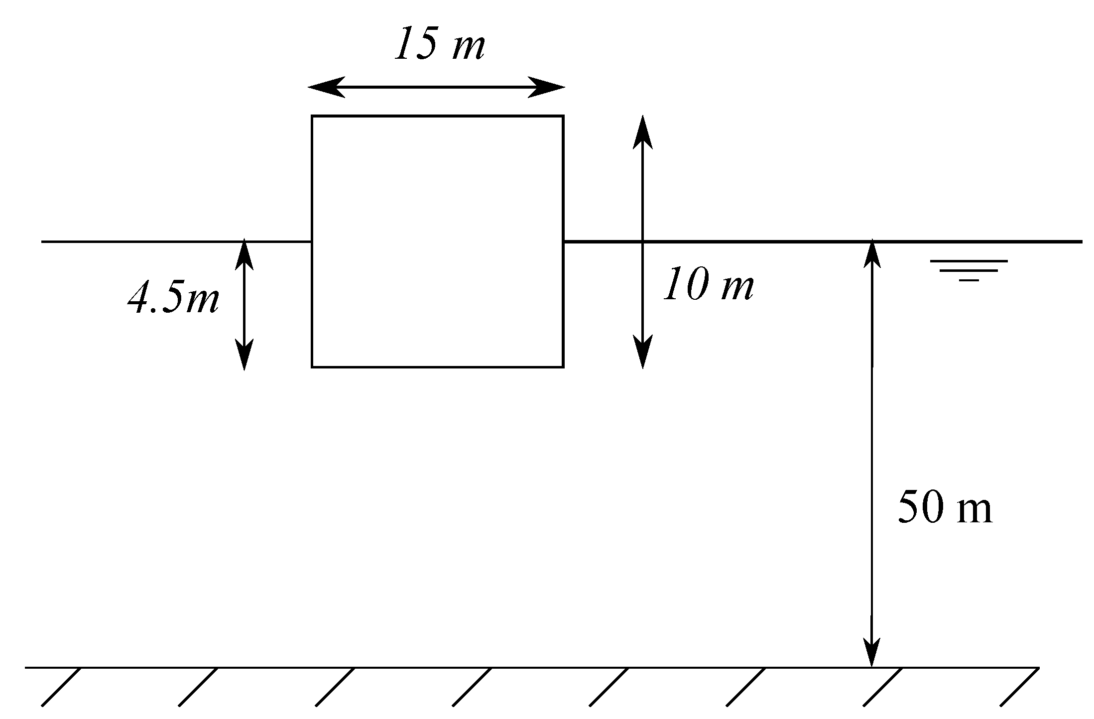
The case study is a simple vertical point-absorber cylinder, oscillating in heave (Figure 1) with the properties listed in

Table 2. Properties of the WEC. x and y-orthogonal horizontal directions; z-vertical direction (positive upward from the still-water level).

Property	Value
Water depth	50 m
Diameter	15 m
Height	10 m
Draft	4.5 m
Mass	813,387 kg
Center of gravity	−0.7 m
Center of buoyancy	−2.25 m

. Due to the fact that point-absorbers are relatively insensitive to wave direction, in this work, their dynamics are studied assuming a single wave direction.

The characteristics of the WEC were adapted from [39], where a cylinder with a hemispherical cap on the bottom was analyzed. Here, the WEC is a perfect cylinder. The deployment location is offshore Karmøy, Norway, with the wave climate described in Table 1. It is assumed that the sea-states at this location can be accurately represented by a JONSWAP spectrum.

4.2. Resource Evaluation and Operational Windows Selection

The available mean power and energy of the WEC are obtained for the deployment location using (4) and (5) and are displayed in

Table 3. Average power flux (top row) ($\mathrm{k}\mathrm{W} \mathrm{m}$⁻¹) and yearly available energy of the sea states (bottom row) ($\mathrm{k}\mathrm{W}\mathrm{h} \mathrm{m}$⁻¹).

	${\mathit{T}}_{\mathbf{z}}$ (s)
${\mathit{H}}_{\mathbf{s}}$	3.75	4.25	4.75	5.25	5.75	6.25	6.75	7.25	7.75	8.25
0.75	1	1	2	2	2	2	2	2	2	3
	0	48	160	236	178	123	38	0	0	0
1.25	3	4	4	5	5	6	6	6	7	7
	29	1626	2114	2542	2065	2098	632	170	0	0
1.75	7	7	8	9	10	11	12	13	14	14
	0	455	4434	7713	6424	4974	2273	888	119	0
2.25	11	12	14	15	17	18	19	21	22	24
	0	0	120	4250	9746	8064	2732	1284	588	0
2.75	16	18	20	23	25	27	29	31	33	36
	0	0	0	198	5215	11,810	2806	1644	586	312
3.25	23	26	29	32	35	38	41	44	47	50
	0	0	0	0	304	5278	6057	2679	2454	871
3.75	30	34	38	42	46	50	54	58	62	66
	0	0	0	0	0	439	4269	2547	1634	580
4.25	39	44	49	54	59	64	70	75	80	85
	0	0	0	0	0	0	0	3272	2099	745
4.75	48	55	61	68	74	80	87	93	100	106
	0	0	0	0	0	0	0	0	2621	930
5.25	59	67	75	82	90	98	106	114	122	130
	0	0	0	0	0	0	0	0	0	1136

. In order to harness the total available energy at the location, the device needs to be able to operate in all sea states. However, to achieve this, the device has to be designed to withstand extreme sea states. This, in turn, leads to higher device cost and inefficient operation at the moderate sea states, which are the most energetic ones, due to it being over-designed for this operating range. As can be seen in Table 3, the most energetic sea states are located in the center of the scatter diagram. Furthermore, the sea states with $T_{\mathrm{z}}$ values between $7.25$ $\mathrm{s}$ and $8.25$ $\mathrm{s}$ and $H_{\mathrm{s}}$ values between $4.25$ $\mathrm{m}$ and $5.25$ $\mathrm{m}$ have relatively high power levels (13% to 96% more powerful than for $T_{\mathrm{z}}=8.25 \mathrm{s},H_{\mathrm{s}}=3.75 \mathrm{m}$), but their combined energy is less than 9% of the total. Therefore, these sea states are considered as extreme cases, where it is not feasible to operate the WEC. Based on this, the cut-off $T_{\mathrm{z}}$ value is selected to be $8.25$ $\mathrm{s}$, and the cut-off $H_{\mathrm{s}}$ value is $3.75$ $\mathrm{m}$. This is similar to the criteria selected in [25] to define operational sea states, excluding the more severe sea states that accounted for less than 10% of the available energy. It is to be noted that at this design stage, this decision of the operational sea states is preliminary; in more advanced design stages, these conditions can be adjusted when the specifications of the WEC are more accurately known.

As for the PTO damping, two scenarios will be tested:

• a realistic scenario with a PTO damping value for each sea state, maximizing the extracted energy in that sea state;
• a simplified scenario with a PTO damping value that maximizes the total extracted energy when the damping is the same for all sea states.

The damping coefficients were obtained using simple optimization algorithms.

4.3. Device Hydrodynamics and Power Estimation

As mentioned above, in order to determine the extracted energy, the PTO damping coefficient is required. In this work, one realistic and one simplified approach are considered for obtaining the PTO damping coefficient. For the realistic scenario, the PTO damping coefficient is optimized for each sea state, i.e., to extract the maximum energy at each sea state. In spite of being more laborious, this approach represents a case similar to a real-life control strategy of a WEC. In turn, the simplified approach utilizes a single PTO damping coefficient that maximizes the total extracted energy from all sea states. The extracted energy from the simplified approach is lower than that in the realistic approach, but the calculation is more time efficient. The discrepancies between the two approaches are quantified in this work, and their validity for pre-design is assessed.

The hydrodynamic data for the device are obtained in ANSYS AQWA (https://www.ansys.com/training-center/course-catalog/structures/introduction-to-hydrodynamic-analysis-with-ansys-aqwa#tab1-1, accessed on 1 September 2024). A maximization function is used to determine the PTO damping coefficients based on the hydrodynamic coefficients computed earlier and integrating (7) using the trapezoidal rule. The optimal PTO coefficient for each sea state is obtained via the iteration of $b_{\mathrm{pto}}$ in (7) until the maximum average power for each sea state is reached. Similarly, the damping coefficient for the simplified scenario is obtained by maximizing the total annual extracted energy. The obtained values of the PTO damping coefficients are presented in

Table 4. PTO damping coefficients ($\mathrm{N}\mathrm{s} \mathrm{m}$⁻¹).

${\mathit{T}}_{\mathbf{z}}$ (s)	Realistic Scenario ${\mathit{b}}_{\mathbf{pto}}$	Simplified Scenario ${\mathit{b}}_{\mathbf{pto}}$
3.75	346,019
4.25	354,658
4.75	411,232
5.25	504,835
5.75	632,881	739,669
6.25	788,322
6.75	960,175
7.25	1,138,982
7.75	1,319,045
8.25	1,497,591

, and the values of the extracted power and energy are presented in

Table 5. Average extracted power estimated using time-domain analysis for the realistic scenario (top row) and for the simplified scenario (bottom row) ($\mathrm{k}\mathrm{W}$).

	${\mathit{T}}_{\mathbf{z}}$ (s)
${\mathit{H}}_{\mathbf{s}}$	3.75	4.25	4.75	5.25	5.75	6.25	6.75	7.25	7.75	8.25
0.75	0	5	6	7	8	9	9	0	0	0
	0	4	6	7	8	9	9	0	0	0
1.25	8	13	18	21	23	24	25	26	0	0
	7	12	16	20	22	24	25	25	0	0
1.75	0	26	35	40	44	47	49	51	52	0
	0	23	32	39	44	47	48	48	48	0
2.25	0	0	57	66	73	77	81	84	86	0
	0	0	52	64	72	77	80	80	79	0
2.75	0	0	0	99	109	116	122	126	129	132
	0	0	0	97	108	116	119	119	118	114
3.25	0	0	0	0	152	162	169	176	180	184
	0	0	0	0	152	161	166	167	165	160
3.75	0	0	0	0	0	216	226	234	239	244
	0	0	0	0	0	215	222	222	219	213

.

The time-domain simulations were performed in WEC-Sim [40]. The results of the estimated average power for the realistic and simplified scenarios are presented in Table 5.

It can be observed from Table 5 that the values of the average extracted power in both scenarios are not drastically different, which indicates that the simplified approach can be used for the initial appraisal and pre-design of the WEC.

5. Determination of the Rated Power

In addition to the mean power, the peak power ($P_{max}$) and RMS power ($P_{\mathrm{rms}}$) values are important parameters for dimensioning the WEC. The values of RMS and peak extracted power, estimated using time-domain simulations, are presented in

Table 6. RMS power estimated using time-domain analysis for the realistic scenario (top row) and for the simplified scenario (bottom row) ($\mathrm{k}\mathrm{W}$).

	${\mathit{T}}_{\mathbf{z}}$ (s)
${\mathit{H}}_{\mathbf{s}}$	3.75	4.25	4.75	5.25	5.75	6.25	6.75	7.25	7.75	8.25
0.75	0	8	11	13	14	15	16	0	0	0
	0	7	10	13	14	15	16	0	0	0
1.25	14	23	31	36	39	41	43	44	0	0
	12	20	27	34	39	42	43	43	0	0
1.75	0	46	60	70	75	81	85	88	91	0
	0	40	55	68	76	83	83	84	84	0
2.25	0	0	99	115	124	134	140	151	155	0
	0	0	92	111	121	132	142	139	135	0
2.75	0	0	0	172	189	200	217	222	223	233
	0	0	0	167	186	201	209	203	204	193
3.25	0	0	0	0	266	286	295	310	310	311
	0	0	0	0	257	285	289	290	285	275
3.75	0	0	0	0	0	372	377	398	419	431
	0	0	0	0	0	383	392	379	376	366

and

Table 7. Peak power estimated using time-domain analysis for the realistic scenario (top row) and for the simplified scenario (bottom row) ($\mathrm{k}\mathrm{W}$).

	${\mathit{T}}_{\mathbf{z}}$ (s)
${\mathit{H}}_{\mathbf{s}}$	3.75	4.25	4.75	5.25	5.75	6.25	6.75	7.25	7.75	8.2
0.75	0	69	123	121	172	132	164	0	0	0
	0	65	96	127	132	155	122	0	0	0
1.25	151	226	270	339	404	306	339	352	0	0
	114	202	231	284	358	369	431	495	0	0
1.75	0	419	487	755	663	655	940	932	783	0
	0	381	707	680	645	802	718	850	654	0
2.25	0	0	857	978	1127	1238	1169	2288	1546	0
	0	0	936	1055	1020	1191	1664	1621	938	0
2.75	0	0	0	1823	1671	1692	2036	1916	2111	2589
	0	0	0	1923	1465	2032	1978	1649	2102	1343
3.25	0	0	0	0	2706	2813	3277	2978	2994	2895
	0	0	0	0	1959	2714	2327	2748	2226	2542
3.75	0	0	0	0	0	3040	3411	3057	4687	5459
	0	0	0	0	0	4117	3663	3213	3262	2679

, respectively, for the simplified and realistic scenarios.

As it can be observed from Table 5 and Table 7, the ratio of peak to average power of the WEC is considerable, with some cases having a peak power of over 20 times the average power. In Section 4.2, it was mentioned that it is not economically feasible to design a WEC that is able to operate at all sea states, and this is the reason why: having a generator designed for loads that are 20 times the average and rarely occurring will lead to a device that operates at a low efficiency at the low- and mid-power sea states, which are the ones that contribute most to the annual energy capture [41]. Moreover, the size and cost of such a generator will be substantial. In order to achieve a generator design with a balanced energy density, power curtailment is introduced.

From Table 5 with the estimated mean power and Table 6 for the RMS power, it can be seen that the two values are fairly similar. This indicates that the RMS power value can be used as a parameter to size the generator that both takes into account the power fluctuations and provides an approximate estimate of the extracted power. In the following analysis, for the sake of simplicity, only the results from simulations for the simplified scenario (using a single PTO coefficient) will be used, since its results are similar to those of the realistic scenario.

Table 6 shows that the RMS power for the most important sea states is in the range of 100 $\mathrm{k}$$\mathrm{W}$ to 360 $\mathrm{k}$$\mathrm{W}$; hence, 360 $\mathrm{k}$$\mathrm{W}$ (the maximum RMS power for the operational sea states, $H_{\mathrm{s}}=3.25 \mathrm{m}$ and $T_{\mathrm{z}}=8.25 \mathrm{s}$), is selected as the rated power. This is a compromise between a significant reduction in the rated power of the generator relative to the peak power and maximization of the power extraction ability of the generator.

To understand the effects of selecting 360 $\mathrm{k}$$\mathrm{W}$ as the rated power, power curtailment simulations were also conducted. The power curtailment is simulated by truncating all power values above 360 $\mathrm{k}$$\mathrm{W}$ to 360 $\mathrm{k}$$\mathrm{W}$. Afterwards, the extracted energy was computed by multiplying the mean of the curtailed power time-series by the probability of the occurrence of each sea state.

The values of the extracted energy with and without curtailment are shown in

Table 8. Extracted energy without power curtailment (top row) and with power curtailment (bottom row) in time-domain simulations for the simplified scenario ($\mathrm{M}\mathrm{W}\mathrm{h}$).

	${\mathit{T}}_{\mathbf{z}}$ (s)
${\mathit{H}}_{\mathbf{s}}$	3.75	4.25	4.75	5.25	5.75	6.25	6.75	7.25	7.75	8.25
0.75	0	0.15	0.61	1.01	0.78	0.53	0.16	0	0	0
	0	0.15	0.61	1.01	0.78	0.53	0.16	0	0	0
1.25	0.06	5	8.12	10.83	8.99	9.01	2.58	0.65	0	0
	0.06	5	8.12	10.83	8.99	9.01	2.58	0.65	0	0
1.75	0	1.4	17.03	32.85	28.11	21.37	9.28	3.39	0.42	0
	0	1.4	16.98	32.68	27.9	21.06	9.2	3.36	0.41	0
2.25	0	0	0.46	18.08	42.46	34.59	11.17	4.88	2.08	0
	0	0	0.45	17.52	41.11	32.93	10.37	4.58	1.96	0
2.75	0	0	0	0.85	22.78	50.85	11.48	6.28	2.06	1
	0	0	0	0.77	20.18	44.03	9.82	5.43	1.79	0.89
3.25	0	0	0	0	1.33	22.61	24.8	10.25	8.68	2.81
	0	0	0	0	1.08	17.29	18.91	7.79	6.65	2.19
3.75	0	0	0	0	0	1.88	17.48	9.74	5.76	1.87
	0	0	0	0	0	1.27	11.63	6.61	3.92	1.29

and

Table 9. Extracted energy without power curtailment, estimated using capture width ($\mathrm{M}\mathrm{W}\mathrm{h}$).

	${\mathit{T}}_{\mathbf{z}}$ (s)
${\mathit{H}}_{\mathbf{s}}$ (m)	3.75	4.2	4.75	5.25	5.75	6.25	6.75	7.25	7.75	8.25
0.75	0	0.21	0.7	1.03	0.77	0.53	0.17	0	0	0
1.25	0.13	7.07	9.2	11.06	8.98	9.13	2.75	0.74	0	0
1.75	0	1.98	19.29	33.55	27.94	21.64	9.89	3.86	0.52	0
2.25	0	0	0.52	18.49	42.4	35.08	11.89	5.59	2.56	0
2.75	0	0	0	0.86	22.69	51.37	12.21	7.15	2.55	1.36
3.25	0	0	0	0	1.32	22.96	26.35	11.65	10.68	3.79
3.75	0	0	0	0	0	1.91	18.57	11.08	7.11	2.52

, where a slight decrease in the extracted energy when curtailment is applied can be seen.

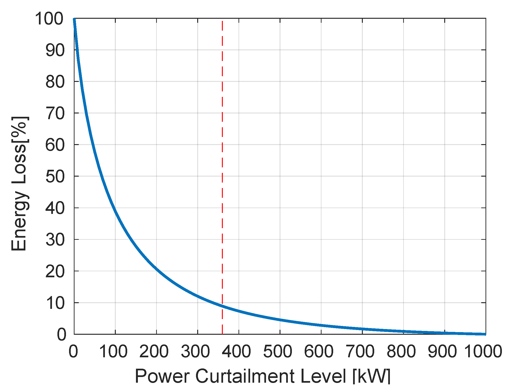
An overall look at the difference in extracted energy is displayed in Figure 2, where the dashed line depicts the selected peak power curtailment level, 360 $\mathrm{k}$$\mathrm{W}$. The consequence of curtailing the peak power at this level, which corresponds to a curtailment of about 87% relative to the peak power, is an energy loss of only about 8.9%. The small impact of this large limitation of the peak power on the extracted energy is caused by the behavior of the instantaneous extracted power. 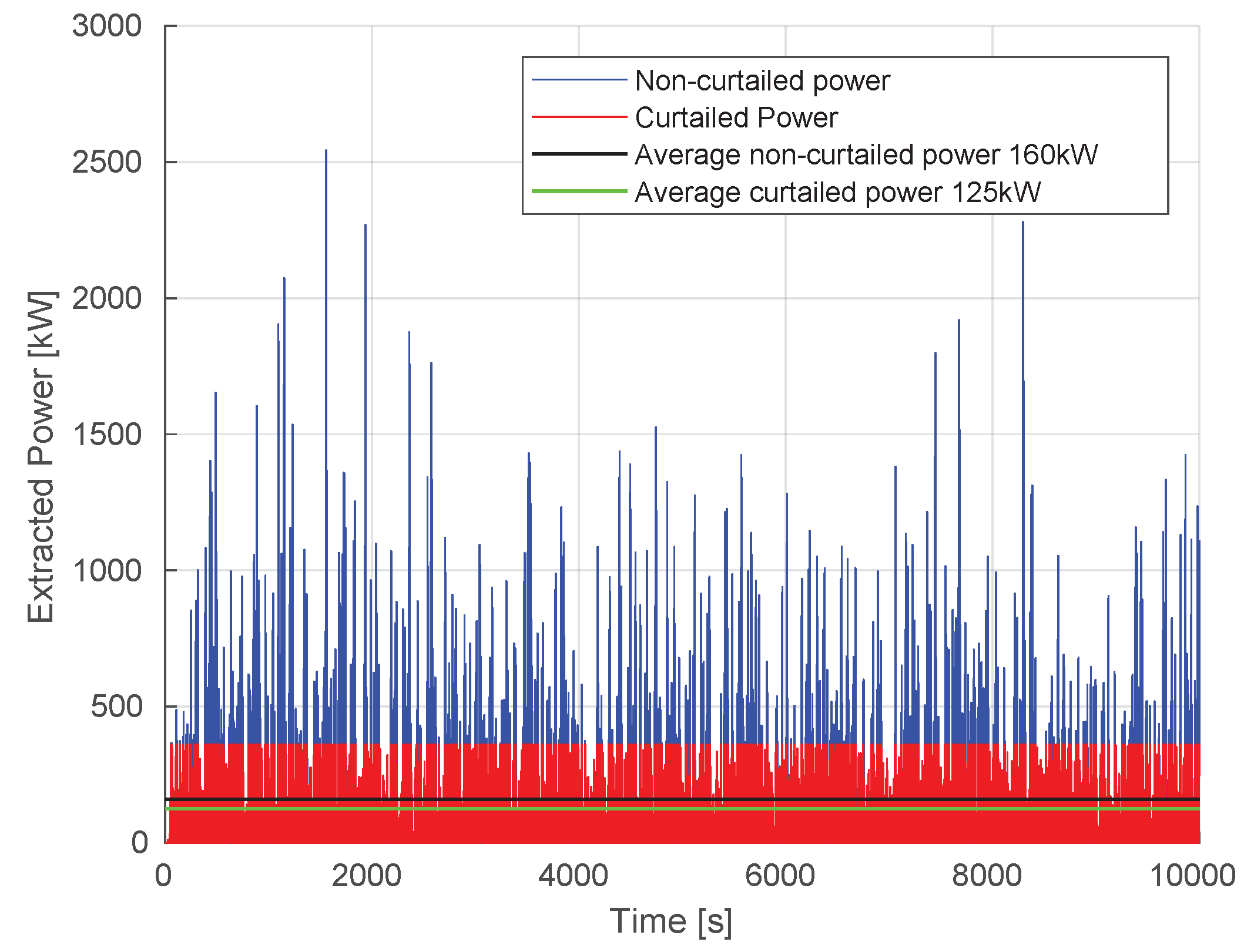Using sea state $H_{\mathrm{s}}=3.25 \mathrm{m}$ and $T_{\mathrm{z}}=8.25 \mathrm{s}$ as an example, the instantaneous power as a function of time and the corresponding average value of the non-curtailed and curtailed cases are shown in Figure 3. Statistically, wave heights have a Rayleigh distribution, with dominance of smaller wave heights over larger ones. As wave power varies quadratically with height, there will be a preponderance of lower power levels, with the occasional appearance of very high (but rare) high-power peaks. As such, curtailing the power at moderate to high power levels will not lead to significant differences in the average power between the curtailed and non-curtailed operations (in this case, the difference is roughly 35 $\mathrm{k}$$\mathrm{W}$). A similar trend is seen in all sea states; hence, the overall energy loss due to peak power curtailment is quite minimal. This is also the reason why the energy loss as a function of curtailment level in Figure 2 is non-linear and decreasing: most energy is transmitted to the device at smaller wave heights, with only occasional larger wave heights appearing.

The proposed methodology provides a means to estimate the rated power, but it does not provide an easy means to estimate the loss of extracted energy as a function of the rated power or curtailment level, or as a function of the control strategy. This subject requires further research.

As a final point in the study of the results of time-domain simulations, hidrodynamic viscous damping was included in the simulation of the dynamics of the WEC (a coefficient of 0.9 acting in the vertical direction, together with a a cross section of $176.7$ m²), with the results presented in

Table 10. Average extracted power estimated using time-domain analysis for the simplified scenario and viscous damping ($\mathrm{k}\mathrm{W}$).

	${\mathit{T}}_{\mathbf{z}}$ (s)
${\mathit{H}}_{\mathbf{s}}$ (m)	3.75	4.25	4.75	5.25	5.75	6.25	6.75	7.25	7.75	8.2
0.75	0	4	6	7	8	8	9	0	0	0
1.25	7	11	16	19	22	23	24	24	0	0
1.75	0	22	30	37	42	45	46	47	46	0
2.25	0	0	50	61	68	74	76	77	76	0
2.75	0	0	0	90	101	109	112	114	113	110
3.25	0	0	0	0	140	151	156	157	155	153
3.75	0	0	0	0	0	198	205	206	206	201

,

Table 11. RMS extracted power estimated using time-domain analysis for the simplified scenario and viscous damping ($\mathrm{k}\mathrm{W}$).

	${\mathit{T}}_{\mathbf{z}}$ (s)
${\mathit{H}}_{\mathbf{s}}$ (m)	3.75	4.25	4.75	5.25	5.75	6.25	6.75	7.25	7.75	8.25
0.75	0	7	10	12	13	15	15	0	0	0
1.25	11	20	27	33	38	40	42	41	0	0
1.75	0	38	51	64	71	78	80	79	81	0
2.25	0	0	86	103	117	125	133	131	132	0
2.75	0	0	0	156	180	186	193	194	188	190
3.25	0	0	0	0	239	251	268	267	262	261
3.75	0	0	0	0	0	331	356	349	358	344

and

Table 12. Extracted energy estimated using time domain analysis and viscous damping ($\mathrm{M}\mathrm{W}\mathrm{h}$).

	${\mathit{T}}_{\mathbf{z}}$ (s)
${\mathit{H}}_{\mathbf{s}}$ (m)	3.75	4.25	4.75	5.25	5.75	6.25	6.75	7.25	7.75	8.25
0.75	0	16	69	112	87	59	17	0	0	0
1.25	7	554	895	1192	1001	996	288	72	0	0
1.75	0	153	1854	3562	3068	2339	1023	375	46	0
2.25	0	0	50	1941	4583	3749	1215	536	227	0
2.75	0	0	0	90	2431	5439	1229	681	225	110
3.25	0	0	0	0	140	2414	2652	1100	930	305
3.75	0	0	0	0	0	198	1841	1029	618	201

.

As expected, the average power, RMS power, and total extracted energy are smaller than for fully linear simulations. However, the difference is not significant. Given the increased simulation time due to the addition of a non-linear term, with results that are not considerably different from fully linear ones, at this stage in the analysis, the benefits of this analysis are judged to be minimal.

6. Expedite Quantification

There is another potential way to quantify the efficiency of a WEC: through its capture width, $\overline{L}$:

$$\begin{array}{c}\hfill \overline{L}={\displaystyle \frac{{\overline{P}}_{\mathrm{pto}}}{\overline{J}}}\end{array}$$

(13)

The units of $\overline{L}$ are those of length; it can be interpreted as the width of a wave with the same average power as that extracted by the device.

The relative capture width, ${\overline{L}}_{\mathrm{r}}$, is the ratio of the capture width to a characteristic length of the WEC. This characteristic length is usually the width, w, of the wave energy converter facing the incoming waves [42]:

$$\begin{array}{c}\hfill {\overline{L}}_{\mathrm{r}}={\displaystyle \frac{{\overline{P}}_{\mathrm{pto}}}{w\overline{J}}}\end{array}$$

(14)

Knowing the device’s width, w, the capture width ratio, ${\overline{L}}_{\mathrm{r}}$ (obtained from reported values, physical and numerical modeling, or from compiled reports) and the available power flux, $\overline{J}$, it is possible to obtain estimates of the power performance of the device, ${\overline{P}}_{\mathrm{pto}}$:

$$\begin{array}{c}\hfill {\overline{P}}_{\mathrm{pto}}={\overline{L}}_{\mathrm{r}}w\overline{J}\end{array}$$

(15)

The main advantage of using this approach over frequency or time domain ones is that the average power generated by the device can be easily estimated without computing hydrodynamic coefficients or running lengthy simulations. Another advantage is that the PTO damping is not present in (15). Even in the simplest case of a linear and constant PTO damping coefficient, it is not easy to provide an early guess for its value for irregular waves, where there is no known optimal solution, bringing further uncertainty to the problem.

For a point-absorber with the dimensions used in this study, ref. [42] reports an expected relative capture width of ${\overline{L}}_{\mathrm{r}}=0.29$, which was, therefore, the value selected for this analysis. Knowing the relative capture width and the device’s diameter, the average extracted power was estimated using (15) and is presented in

Table 13. Average extracted power estimated using capture width ($\mathrm{k}\mathrm{W}$).

	${\mathit{T}}_{\mathbf{z}}$ (s)
${\mathit{H}}_{\mathbf{s}}$ (m)	3.75	4.25	4.75	5.25	5.75	6.25	6.75	7.25	7.75	8.25
0.75	0	6	7	7	8	9	9	0	0	0
1.25	15	16	18	20	22	24	26	28	0	0
1.75	0	32	36	40	44	47	51	55	59	0
2.25	0	0	60	66	72	78	85	91	97	0
2.75	0	0	0	98	108	117	127	136	145	155
3.25	0	0	0	0	151	164	177	190	203	216
3.75	0	0	0	0	0	218	235	253	270	288

.

After studying Table 5 and Table 13, it is seen that the power estimates of the two methods, time-domain and relative capture width, do not vary significantly. The discrepancy in the analysis, presented in

Table 14. Discrepancy between mean power estimated using time-domain analysis for the realistic scenario estimated using capture width (row 1) and for the simplified scenario estimated using capture width (row 2) (%).

	${\mathit{T}}_{\mathbf{z}}$ (s)
${\mathit{H}}_{\mathbf{s}}$	3.75	4.25	4.75	5.25	5.75	6.25	6.75	7.25	7.75	8.25	Mean
0.75	0	22.8	4.3	0.7	1.0	0.9	4.2	0	0	0
	0	41.3	13.7	2.3	0.4	1.3	5.9	0	0	0
1.25	81.8	23.0	4.3	0.9	1.1	1.0	4.4	8.4	0	0
	113.6	41.6	13.3	2.1	0.1	1.3	6.8	13.7	0	0
1.75	0	23.2	4.6	1.0	0.4	1.2	4	7.8	13.3	0
	0	41	13.3	2.2	0.6	1.3	6.5	13.7	23.5	0
2.25	0	0	4.6	0.8	1.2	1.4	4.1	8.5	12.5	0	3.6
	0	0	13.9	2.2	0.2	1.4	6.4	14.4	23.3	0	6.7
2.75	0	0	0	1.0	1.1	1.2	4.1	7.9	13	17.6
	0	0	0	2	0.4	1	6.3	14	23.6	35.1
3.25	0	0	0	0	0.7	1.0	4.4	8.1	12.6	17.4
	0	0	0	0	0.9	1.6	6.2	13.7	23.1	35.2
3.75	0	0	0	0	0	0.8	4.4	8.2	13.2	18.1
	0	0	0	0	0	1.3	6.2	13.8	23.5	34.8

, is acceptable. For the most energetic sea state, the difference between estimates using capture width and using time-domain analysis is about 1% ($H_{\mathrm{s}}$ = $2.75$ $\mathrm{m}$, $T_{\mathrm{z}}$ = $6.25$ $\mathrm{s}$), and it goes up to about 5% for the other energetic sea states. For the least-energetic sea states, where small absolute differences lead to very large relative discrepancies, the differences can be about 100%, such as for sea state $H_{\mathrm{s}}$ = $1.25$ $\mathrm{m}$, $T_{\mathrm{z}}$ = $3.75$ $\mathrm{s}$; however, these sea states have an almost negligible contribution to the total extracted energy (some with less than 1%). The discrepancy is also dependent on the approach used to model the control of the wave energy converter: the difference between the capture width method and the realistic scenario is about half of the difference between using the capture width method and the simplified scenario. The estimated mean discrepancy, obtained by weighting the discrepancy in each sea state by its probability of occurrence, varies by about 3.6% when comparing the capture width method with estimates for the realistic scenario and 7.0% when comparing the capture width ratio with estimates for the simplified scenario.

By comparing Table 5 with Table 6 and Table 7, it can be seen that there is an approximately constant ratio between $P_{\mathrm{rms}}$ and ${\overline{P}}_{\mathrm{pto}}$ of $1.7$ and a ratio between $P_{\max }$ and ${\overline{P}}_{\mathrm{pto}}$ of 17. This approximately constant ratio demonstrates that we can bypass lengthy time-domain simulations by obtaining estimates of $P_{\mathrm{rms}}$ and of $P_{\max }$ from ${\overline{P}}_{\mathrm{pto}}$ via multiplication by a suitable coefficient. In this work, we demonstrated this for a simple point-absorber. Further work is required to determine how general and useful these coefficients can be for other types of devices.

Up to the current section, all calculations and estimates were based on the geometrical, mechanical, and other physical properties of the device, so they can be generalized to the whole range of existing wave energy converters (assuming the underlying theories to be valid). On the other hand, the application of the relative capture width is based on the few test data that are not classified by WEC developers, and this is rather empiric. As such, although it is promising for axisymmetric point absorbers, it needs to be validated for other types of devices.

7. Conclusions

A method for the selection of the rated power of the electrical generator of a heaving point-absorber wave energy converter was proposed. The proposed methodology used linear potential flow theory and linear power take-off to model the wave energy converter. Due to the highly irregular power profile characteristic of ocean waves (peak power at a given sea state can be around 20 times the average power), peak power curtailment is introduced in order to select a suitable rated power value for the generator unit. The rated power of the generator, set at 360 $\mathrm{k}$$\mathrm{W}$, is based on the root mean square power extracted by the wave energy converter at its deployment location when working without any restriction. Selecting the rated power as the RMS power of the most powerful operational sea states leads to a good compromise between rated power and energy loss. This curtailment level limits the peak power by as much as about 87%, but it results in a reduction in extracted energy of only 8.9%. Eliminating the over-design of the generator can result in significant cost savings without significant loss of revenue.

In addition, it is also conjectured that a simpler method to obtain the RMS and peak power of the wave energy converter can be developed, since there seems to be a constant ratio between the average power and the RMS and peak power. For the case of a heaving point-absorber deployed offshore Karmøy studied here, the ratio of RMS to average power and the ratio of peak power to mean power were found to be roughly 1.7 and 17, respectively. This simplified method was estimated to have a discrepancy in time-domain calculations of between 3.6% and 7.0% (depending on how detailed the time-domain simulations are). However, further research is required on the general applicability of this method. For future steps, it is suggested that these conclusions are verified for different locations and, afterwards, adjusted to the wide variety of wave energy converters in existence. Finally, it is suggested that, as full-scale prototype data are released, the methodology is fine-tuned to real-world data.

In addition to the suggestions for future development on the usage of the capture width ratio as a design tool, we suggest a deeper investigation into non-linear effects. Current research and our own results show that non-linearities might lead to smaller energy extraction when compared with linear estimates. However, these effects will depend strongly on the type and location of device: onshore devices will be more affected by non-linear effects than offshore point absorbers, for example, whose loading in operating conditions can be considered to be linear. The inclusion of non-linear effects needs to be reasonable: adding non-linear terms will improve the quality of the results, but the goal of this work is to obtain good enough estimates of power for a pre-design stage and not the time-consuming exact modeling of the device.

References

- Schoen, M.P.; Hals, J.; Moan, T. Wave Prediction and Robust Control of Heaving Wave Energy Devices for Irregular Waves. IEEE Trans. Energy Convers. 2011, 26, 627–638. [Google Scholar] [CrossRef]
- Wu, F.; Zhou, N.; Ju, P.; Zhang, X. Wind–Wave Coupling Model for Wave Energy Forecast. IEEE Trans. Sustain. Energy 2019, 10, 586–595. [Google Scholar] [CrossRef]
- Fusco, F.; Ringwood, J.V. Short-Term Wave Forecasting for Real-Time Control of Wave Energy Converters. IEEE Trans. Sustain. Energy 2010, 1, 99–106. [Google Scholar] [CrossRef]
- Blanco, M.; Lafoz, M.; Ramirez, D.; Navarro, G.; Torres, J.; García-Tabares, L. Dimensioning of Point Absorbers for Wave Energy Conversion by Means of Differential Evolutionary Algorithms. IEEE Trans. Sustain. Energy 2019, 10, 1076–1085. [Google Scholar] [CrossRef]
- Sproul, A.; Weise, N. Analysis of a Wave Front Parallel WEC Prototype. IEEE Trans. Sustain. Energy 2015, 6, 1183–1189. [Google Scholar] [CrossRef]
- Hazra, S.; Bhattacharya, S. Modeling and Emulation of a Rotating Paddle Type Wave Energy Converter. IEEE Trans. Energy Convers. 2018, 33, 594–604. [Google Scholar] [CrossRef]
- Tindall, C.; Xu, M. Optimising a Wells-turbine-type wave energy system. IEEE Trans. Energy Convers. 1996, 11, 631–635. [Google Scholar] [CrossRef]
- Baker, N.J.; Raihan, M.A.H.; Almoraya, A.A. A Cylindrical Linear Permanent Magnet Vernier Hybrid Machine for Wave Energy. IEEE Trans. Energy Convers. 2019, 34, 691–700. [Google Scholar] [CrossRef]
- Mueller, M.A.; Burchell, J.; Chong, Y.C.; Keysan, O.; McDonald, A.; Galbraith, M.; Echenique Subiabre, E.J.P. Improving the Thermal Performance of Rotary and Linear Air-Cored Permanent Magnet Machines for Direct Drive Wind and Wave Energy Applications. IEEE Trans. Energy Convers. 2019, 34, 773–781. [Google Scholar] [CrossRef]
- Polinder, H.; Mecrow, B.C.; Jack, A.G.; Dickinson, P.G.; Mueller, M.A. Conventional and TFPM linear generators for direct-drive wave energy conversion. IEEE Trans. Energy Convers. 2005, 20, 260–267. [Google Scholar] [CrossRef]
- Alberdi, M.; Amundarain, M.; Garrido, A.J.; Garrido, I.; Casquero, O.; De la Sen, M. Complementary Control of Oscillating Water Column-Based Wave Energy Conversion Plants to Improve the Instantaneous Power Output. IEEE Trans. Energy Convers. 2011, 26, 1021–1032. [Google Scholar] [CrossRef]
- Tedeschi, E.; Carraro, M.; Molinas, M.; Mattavelli, P. Effect of Control Strategies and Power Take-Off Efficiency on the Power Capture From Sea Waves. IEEE Trans. Energy Convers. 2011, 26, 1088–1098. [Google Scholar] [CrossRef]
- Garcia-Rosa, P.B.; Ringwood, J.V. On the Sensitivity of Optimal Wave Energy Device Geometry to the Energy Maximizing Control System. IEEE Trans. Sustain. Energy 2016, 7, 419–426. [Google Scholar] [CrossRef]
- García-Violini, D.; Peña-Sanchez, Y.; Faedo, N.; Ringwood, J.V. An Energy-Maximising Linear Time Invariant Controller (LiTe-Con) for Wave Energy Devices. IEEE Trans. Sustain. Energy 2020, 11, 2713–2721. [Google Scholar] [CrossRef]
- M’zoughi, F.; Bouallègue, S.; Garrido, A.J.; Garrido, I.; Ayadi, M. Stalling-Free Control Strategies for Oscillating-Water-Column-Based Wave Power Generation Plants. IEEE Trans. Energy Convers. 2018, 33, 209–222. [Google Scholar] [CrossRef]
- Kovaltchouk, T.; Blavette, A.; Aubry, J.; Ahmed, H.B.; Multon, B. Comparison Between Centralized and Decentralized Storage Energy Management for Direct Wave Energy Converter Farm. IEEE Trans. Energy Convers. 2016, 31, 1051–1058. [Google Scholar] [CrossRef]
- Yegna Narayanan, S.S.; Murthy, B.K.; Sridhara Rao, G. Dynamic analysis of a grid-connected induction generator driven by a wave-energy turbine through hunting networks. IEEE Trans. Energy Convers. 1999, 14, 115–120. [Google Scholar] [CrossRef]
- Kiran, D.R.; Palani, A.; Muthukumar, S.; Jayashankar, V. Steady Grid Power From Wave Energy. IEEE Trans. Energy Convers. 2007, 22, 539–540. [Google Scholar] [CrossRef]
- Coiro, D.P.; Troise, G.; Calise, G.; Bizzarrini, N. Wave energy conversion through a point pivoted absorber: Numerical and experimental tests on a scaled model. Renew. Energy 2016, 87, 317–325. [Google Scholar] [CrossRef]
- Freeman, K. Numerical Modelling and Control of an Oscillating Water Column Wave Energy Converter. Ph.D. Thesis, Plymouth University, Plymouth, UK, 2014. [Google Scholar]
- Reyes, C.C.M.; Walker, M.; Huang, Z.; Cross, P. A Dual-Function Design of an Oscillating Water Column Integrated with a Slotted Breakwater: A Wave Flume Study. Energies 2024, 17, 3848. [Google Scholar] [CrossRef]
- Martinelli, L.; Zanuttigh, B.; Kofoed, J.P. Selection of design power of wave energy converters based on wave basin experiments. Renew. Energy 2011, 36, 3124–3132. [Google Scholar] [CrossRef]
- Oh, J.S.; Kim, J.D.; Lee, J.H.; Park, H.I.; Komatsu, T. Design and analysis of wave energy converter for a buoy. J. Mech. Sci. Technol. 2007, 21, 2005–2010. [Google Scholar] [CrossRef]
- Ruellan, M.; BenAhmed, H.; Multon, B.; Josset, C.; Babarit, A.; Clement, A. Design Methodology for a SEAREV Wave Energy Converter. IEEE Trans. Energy Convers. 2010, 25, 760–767. [Google Scholar] [CrossRef]
- Ciappi, L.; Simonetti, I.; Bianchini, A.; Cappietti, L.; Manfrida, G. Application of integrated wave-to-wire modelling for the preliminary design of oscillating water column systems for installations in moderate wave climates. Renew. Energy 2022, 194, 232–248. [Google Scholar] [CrossRef]
- Henriques, J.; Portillo, J.; Sheng, W.; Gato, L.; Falcão, A. Dynamics and control of air turbines in oscillating-water-column wave energy converters: Analyses and case study. Renew. Sustain. Energy Rev. 2019, 112, 571–589. [Google Scholar] [CrossRef]
- Pecher, A.; Kofoed, J.P. Introduction. In Handbook of Ocean Wave Energy; Springer Nature: Cham, Switzerland, 2017; Chapter 1. [Google Scholar]
- Tokat, P. Design and Evaluation of a Permanent Magnet Generator for Wave Power Applications; Department of Energy and Environment, Electric Power Engineering, Chalmers University of Technology: Göteborg, Sweden, 2015. [Google Scholar]
- Falnes, J. A review of wave-energy extraction. Mar. Struct. 2007, 20, 185–201. [Google Scholar] [CrossRef]
- Barstow, S.; Mollison, D.; Cruz, J. The Wave Energy Resource. In Ocean Wave Energy—Current Status and Future Perspectives, 1st ed.; Cruz, J., Ed.; Springer: Berlin/Heidelberg, Germany, 2008; Chapter 4. [Google Scholar] [CrossRef]
- U.S. Army Corps of Engineers. Part II—Chapter 1—Water Wave Mechanics. In Coastal Engineering Manual EM 1110-2-1100, Change 1 ed.; U.S. Army Corps of Engineers: Washington, DC, USA, 2002; Chapter II-1. [Google Scholar]
- Bergdahl, L. Wave-Induced Loads and Ship Motions; Chalmers University of Technology: Göteborg, Sweden, 2010; p. 188. [Google Scholar]
- Beels, C.; Henriques, J.C.C.; De Rouck, J.; Pontes, M.T.; De Backer, G.; Verhaeghe, H. Wave energy resource in the North Sea. In Proceedings of the 7th European Wave and Tidal Energy Conference, Porto, Portugal, 11–14 September 2007. [Google Scholar]
- Falnes, J. Ocean Waves and Oscillating Systems: Linear Interactions Including Wave-Energy Extraction; Cambridge University Press: Cambridge, UK, 2002. [Google Scholar]
- Newland, D.E. An Introduction to Random Vibrations, Spectral and Wavelet Analysis, 3rd ed.; Dover Publication, Inc.: Mineola, NY, USA, 1993; pp. 29–477. [Google Scholar]
- Saulnier, J.B.; Ricci, P.; Clément, A.H.; Falcão, A.F.D.O. Mean Power Output Estimation of WECs in Simulated Sea. In Proceedings of the Eighth European Wave and Tidal Energy Conference, Uppsala, Sweden, 7–11 September 2009. [Google Scholar]
- Cummins, W.E. The Impulse Response Function and Ship Motions; Technical Report; David Taylor Model Basin: Washington, DC, USA, 1962. [Google Scholar]
- Newman, J.N. Marine Hydrodynamics; The MIT Press: Cambridge, MA, USA, 1977; p. 402. [Google Scholar]
- Cerveira, F.; Fonseca, N.; Pascoal, R. Mooring system influence on the efficiency of wave energy converters. Int. J. Mar. Energy 2013, 3–4, 65–81. [Google Scholar] [CrossRef]
- National Renewable Energy Laboratory and Sandia Corporation. WEC-Sim (Wave Energy Converter SIMulator)—WEC-Sim Documentation; National Renewable Energy Laboratory and Sandia Corporation: Albuquerque, NM, USA, 2015. [Google Scholar]
- Tokat, P.; Thiringer, T. Sizing of IPM Generator for a Single Point Absorber Type Wave Energy Converter. IEEE Trans. Energy Convers. 2018, 33, 10–19. [Google Scholar] [CrossRef]
- Babarit, A.; Hals, J. On the maximum and actual capture width ratio of wave energy converters. In Proceedings of the 9th European Wave and Tidal Energy Conference, Southampton, UK, 5–9 September 2011. [Google Scholar]
Figure 1.
Set-up of the wave energy converter.
Figure 2.
Percentage of energy loss dependent on the peak power curtailment.
Figure 3.
Instantaneous and average power for curtailed peak power for and .