Abstract
The increasing interest in employing wide-bandgap (WBG) drive systems has brought about very high power, high-frequency inverters enjoying switching frequencies up to hundreds of kilohertz. However, voltage surges with steep fronts, caused by turning semiconductor switches on/off in inverters, travel through the cable and are reflected at interfaces due to impedance mismatches, giving rise to overvoltages at motor terminals and in motor windings. The phenomena typically associated with these repetitive overvoltages are partial discharges and heating in the insulation system, both of which contribute to insulation system degradation and may lead to premature failures. In this article, taking the mentioned challenges into account, the repetitive transient overvoltage phenomenon in WBG drive systems is evaluated at motor terminals and in motor windings by implementing a precise multiconductor transmission line (MCTL) model in the time domain considering skin and proximity effects. In this regard, first, a finite element method (FEM) analysis is conducted in COMSOL Multiphysics to calculate parasitic elements of the motor; next, the vector fitting approach is employed to properly account for the frequency dependency of calculated elements, and, finally, the model is developed in EMTP-RV to assess the transient overvoltages at motor terminals and in motor windings. As shown, the harshest situation occurs in turns closer to motor terminals and/or turns closer to the neutral point depending on whether the neutral point is grounded or floating, how different phases are connected, and how motor phases are excited by pulse width modulation (PWM) voltages.
1. Introduction
The advent of wide-bandgap (WBG) devices, silicon carbide (SiC) and gallium nitride (GaN), brought about very high power, fast switching power electronic converters which resulted in inverters with switching frequencies up to hundreds of kilohertz when accompanied by soft-switching techniques; these inverters enjoy substantially higher specific power and energy than traditional silicon (Si)-based inverters, while their electrical features are not compromised. However, voltage surges with steep fronts, caused by turning semiconductor switches on/off in inverters, travel through transmission cables and are reflected at interfaces due to impedance mismatches, which gives rise to local overvoltages [1]. Additionally, the high slew rates of WBG devices that can reach as high as 100 kV/μs lead to non-uniform voltage distribution in motor windings, where the peak voltage usually occurs in the first turns of the stator winding and/or turns closer to the neutral point [2]. The overvoltage at motor terminals can reach twice as much as that at inverter terminals, known as the doubled voltage effect, and even higher. These repetitive overvoltages at motor terminals and stator windings also cause partial discharges inside motor windings and adversely affect electric machines’ insulation capability, which leads to dielectric breakdown and premature failures, the most common failure in industrial electric machines.
The overvoltage problem of Si-based drive systems has been discussed extensively since the 1980s, focusing on adjustable speed drives (ASD), and models have been developed to understand the phenomenon, [3,4,5], to name a few. The theory for multiconductor transmission line (MCTL) and coil modeling was developed in [6,7], which was the basis for many subsequent papers. The initially proposed transmission line theory considers only static field analysis methods for per unit resistances, inductances, and capacitances along the cable and assumes a transverse electromagnetic (TEM) or a quasi-TEM propagation mode along the cable [8,9]. Very high switching frequency and fast transition times in WBG devices, which can be as low as 10 ns, pose serious challenges when designing the motor and, thus, must be considered when designing drives’ insulation systems. Determining the factors affecting peak terminal overvoltage are motor and cable surge impedances, cable length, cable damping, rise time and magnitude of the drive pulse, and spacing of pulse width modulation (PWM) pulses [10]. The effect of voltage waveforms on motor performance is considered in [11], where electrical, thermal, mechanical, and environmental stresses are recognized as primary stresses that the stator windings face and are discussed in detail. In [12], a model assuming partially lumped and partially distributed parameters is developed, and then the authors in [13] proposed a universal model for three-phase induction motors to simultaneously consider common mode, differential mode, and bearing circuit models to cope with the overvoltage issue. The effect of stress grading regions in coils is also considered in [14], and transient overvoltage, electric field, and heat generation are modeled in machine coils. In [15], the authors aimed to calculate the maximum transient overvoltage and current in interior parts of a cable connecting a WBG inverter to a motor, while the electric field distributions in air cavities that may occur inside the insulation of motor windings are assessed in detail in [16] to provide a reference point in analyzing the impact of PWM voltage waveforms on partial discharge behavior in WBG drives. The inter-turn voltage stress of hairpin windings is considered in [17], and a high-frequency equivalent circuit model considering parasitic parameters is proposed to analyze the overvoltage phenomenon. In [18], a review of overvoltage at motor terminals is presented and a linear equivalent model is proposed.
None of the papers mentioned above considered the frequency-dependent behavior of parasitic parameters in motor windings. Also, it is of great significance to consider the high slew rates of WBG devices and capture the high-frequency behavior of the motor windings which may be up to megahertz order of magnitude. Therefore, this article aims to represent the MCTL model of stator windings considering skin and proximity effects, and, at the same time, models the frequency-dependent behavior of parasitic elements of the motor. The overvoltage phenomenon in WBG drive systems is discussed and analyzed in this article, and the non-uniform voltage distribution in motor windings is precisely evaluated by developing an MCTL model of stator windings in the time domain considering skin and proximity effects. In this regard, using a 60 kW permanent magnet synchronous motor (PMSM) adapted for an electric vehicle (EV), the step-by-step procedure to arrive at the model is presented in detail in the following sections. Therefore, this presented article is organized as follows. In Section 2, the overvoltage phenomenon in WBG drive systems is discussed and the overvoltage at motor terminals is analyzed. This provides the context to represent the developed MCTL model of motor windings in Section 3; this section aims to represent the methodology to model the motor windings in detail. Note that neither the modeling of the inverter nor the cable connecting the inverter and the motor is not recognized as the aims of this presented article. In Section 4, steps to arrive at the MCTL model are discussed in detail; firstly, a finite element method (FEM) model of stator windings is implemented in COMSOL Multiphysics to compute parasitic elements of the motor considering skin and proximity effects; next, rational approximation of frequency domain responses resulted from the FEM simulation is done in MATLAB to properly representing the frequency-dependent behavior of computed parasitic elements; finally, the MTCL model of the stator windings is developed in EMTP-RV to analyze the overvoltage phenomenon in motor windings. In Section 5, simulation results are shown and discussed in detail, and, finally, Section 6 sums up the most important concepts presented in the article.
2. Overvoltage Phenomenon in WBG Drive Systems
As shown in Figure 1, a drive system consists of an inverter supplied by a DC voltage source to provide the electrical power, a cable connecting the inverter to the motor, and a motor. The required specific power of motors is different depending on the applications; a 0.1–0.5 kW/kg specific power suffices for industrial motors, while specific powers of 1–3 kW/kg and above 10 kW/kg are recognized in the literature for EVs and passenger-class electrified aircraft, respectively [19,20,21,22]. Potential motor types for EVs include DC series motor, brushless DC motor (BLDC), permanent magnet synchronous motor (PMSM), induction motor (IM), and switched reluctance motor (SRM). Compared to BLDC motors, PMSMs are supplied by an AC source, have permanent magnets in their rotors, and are usually designed with three phases. Both BLDC motors and PMSMs enjoy high traction characteristics efficiency, while the major problem with IMs and SRMs is the complexity of their control schemes. The only well-known EV employing IMs is the Tesla Model S, while almost all designed and implemented motors for EVs are PMSMs, e.g., motors for the Toyota Prius, Chevrolet Bolt EV, Nissan Leaf, etc. Therefore, the overvoltage phenomenon is discussed in this article using an example PMSM adapted for the 2010 Toyota Prius.

Figure 1.
A WBG drive system consisted of the inverter, cable, and electric motor.
2.1. Wide-Bandgap Devices in Power Electronics Converters
There is an increasing interest in employing WBG-based semiconductors in power electronics converters due to their high voltage work capabilities and ability to work at higher temperatures compared to their Si-based counterparts. Above 10 kV SiC and GaN metal-oxide-semiconductor field-effect transistor (MOSFET) and insulated-gate bipolar transistor (IGBT) can operate at > 200 °C without compromising their electric features and are commercially available, while no Si-based semiconductor is found to be able to operate above 6.5 kV. As a result, WBG devices remove the need for designing series/parallel switch structures to achieve higher voltages and currents; and bring about extremely high specific power and energy in power electronics converters [23]. Also, WBG devices are less vulnerable to radiation and enjoy a higher electric breakdown field compared to Si-based semiconductors, and, thus, enjoy a lower on-resistance for a specific breakdown voltage, resulting in reduced chip size and less conduction loss. A detailed discussion of WBG devices falls beyond this article’s scope. Readers may refer to [24,25,26] for extensive discussions of characteristics and benefits, technologies, and emerging applications of WBG devices.
On the other hand, extremely high frequency and high slew rates of WBG devices pose severe challenges and worsen associated challenges to the slew rate of conventional Si-based semiconductors. These challenges include but are not limited to overvoltage problem at motor terminals and in motor windings. Phenomena that are typically associated with these repetitive overvoltages are partial discharges and heating in insulation systems, both of which contribute to insulation system degradation [27,28,29].
2.2. Overvoltage Phenomenon at Motor Terminals
If a single inverter, cable, and motor are assumed, the overvoltage at motor terminals may reach twice as much as that at inverter terminals. As discussed, the voltage peak at motor terminals is affected by several factors, among which the rise time of the generated PWM voltage and the cable length have significant effects and are discussed in this section. For the drive system shown in Figure 1, using the transmission line theory [30], transmitted and reflected waves at motor terminals can be expressed by Equations (1) and (2), respectively:
where is the DC link voltage, and and are the transmission and reflection coefficients, respectively, and are defined below.
is the surge impedance of the motor and is the surge impedance of the cable. The surge impedance of the cable is defined as
where and are the inductance and capacitance of the cable and can be per unit cable length. Also, the wave propagation velocity () can be defined as:
or:
where and are permeability and permittivity of the dielectric material, respectively. If parameters in the above equations are assumed as below:
- = 1 p.u. to represent the voltage at inverter terminals.
- ≈ 2 and ≈ 1 to represent the worst case; this happens when the surge impedance of the motor is much higher than that of the cable (). = 5000 is assumed in this section. Note that the ratio of 5000 is not necessarily a realistic assumption, and the exact value depends on the motor and the employed cable. In this section, the number is selected to show the maximum possible transient overvoltage and the doubled voltage effect at motor terminals.
- = (1/2) × 3× 108 m/s (half of the speed light), which is a good approximation of the pulse propagation velocity in the cable. For example, if the realistic relative permeability of the cable is assumed to be = 1 and the realistic relative permittivity is assumed to be = 4.5 [31], the wave propagation velocity is calculated as:
It is shown in [32] that the transient voltage peak at motor terminals can reach twice as much as that at inverter terminals with a PWM voltage with rise time ~10–20 ns and a cable length ~2 m. This phenomenon is called the doubled voltage effect. If the drive system shown in Figure 2 is considered, where the motor is replaced by a lumped impedance where , Figure 3 shows the voltage at motor terminals () for cable lengths of = 2 m and = 5 m when supplied by a step voltage with a rise time of = 30 ns and the motor is connected to the inverter through a cable with per unit length resistance 10−5 Ω/m. As shown, for a longer cable, the voltage peak is closer to 2 p.u. and it takes more time to converge to 1 p.u. In addition, although the overvoltage caused by a single inverter does not exceed twice as much as that at inverter terminals, greater overvoltages may exist due to polarity reversal, superposition of two pulses, etc. [18]. Also, Figure 4 shows the first 0.15 μs of voltage waveforms at motor terminals when the motor is supplied by a step voltage with = 30 ns through the cable with lengths = 1, 2, 5, and 10 m. As shown, the higher the cable length, the higher the voltage peak at motor terminals, but as discussed, the peak does not exceed 2 p.u. when a single drive system is assumed. Also, it takes more time for the voltage to converge to 1 p.u. for higher cable lengths.
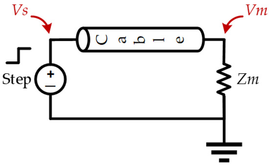
Figure 2.
Simplified motor considered as one lumped resistance connected to a step voltage source through a cable.
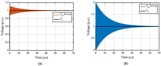
Figure 3.
The voltage at motor terminals () when the motor is fed by a step voltage with = 30 ns through a cable with (a) = 1 m; (b) = 5 m.
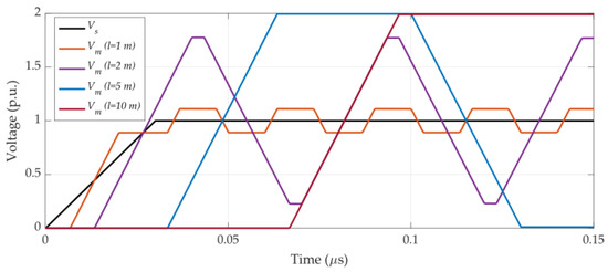
Figure 4.
The first 0.15 μs of voltage waveforms at motor terminals () when the motor is fed by a step voltage with = 30 ns.
As the next simulation, Figure 5 shows the voltage at motor terminals when fed by the inverter through a cable with a per unit length resistance 10−5 Ω/m and length = 2 m and is supplied by step voltages with = 30 and 50 ns. As shown, the voltage peak is greater for the smaller and it takes more time for the voltage to converge to 1 p.u. Also, Figure 6 shows the first 0.15 μs of the voltage at motor terminals when the motor is connected to the inverter through a cable with = 2 m and is supplied by step voltages with different rise times ( = 10, 30, 50, and 150 ns). As shown, the voltage peak is greater for shorter rise times; also, very little overvoltage is seen for = 2 m when = 50, 150 ns, while = 2 p.u. occurs when = 10 ns even with a cable length as short as only 2 m.

Figure 5.
The voltage at motor terminals () when the motor is connected to the inverter through a cable with = 2 m and fed by a step voltage with (a) = 10 ns; (b) = 50 ns.
Figure 6.
Comparison of the first 0.2 μs of voltage at motor terminals () when the motor is connected to the inverter through a cable with = 2 m and fed by a step voltage with various rise times.
A cable with a per unit length resistance of 10−5 Ω/m is assumed above. If the per unit length resistance of the cable is considered 10−4 Ω/m, Figure 7 compares the voltages at motor terminals when the motor is fed by a step voltage with = 10 ns. As expected, when the resistance of the cable is increased, the voltage converges to 1 p.u. in a shorter time and the voltage peak decreases. Note that although 10−4 Ω/m is a realistic number, mentioned resistivities are not necessarily practical numbers and are selected to show the impact of a change in the resistivity of the employed cable.
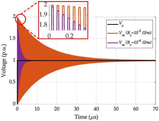
Figure 7.
The voltage at motor terminals () when the motor is connected to the inverter through a cable with = 2 m and fed by a step voltage with = 10 ns.
As shown in this section, peak voltages ~1.5–2 times higher than that at inverter terminals may easily occur when a WBG-based drive is assumed and the rise time of its generated voltage is as low as 10–20 ns. The overvoltage is mainly related to cable characteristics, length, and switching slew rate. The back-and-forth voltage reflection between the inverter and the motor leads to highly repetitive overvoltages where the repetition can be up to megahertz. This should carefully be taken into consideration when designing the insulation system and selecting insulation materials for an electric motor.
2.3. Overvoltage Mitigation Methods
Two general solutions are suggested in the literature to mitigate the overvoltage problem: passive and active filtering. Passive filters include tuning an RLC filter at the output of inverter terminals, the input of the motor terminals, or both [33]. A passive RLC filter was designed for SiC inverters and results were verified using a 75 kW inverter in [34]. Passive filters are less expensive, easier to design, and more robust, but indicating proper values of filter components is challenging. On the other hand, active approaches may translate into providing switches with soft switching techniques, using multiple inverters, designing modified PWM techniques, etc. Since passive filters are typically designed for a specific cable length, they should be redesigned when the cable length is changed or a system with several inverter–motor connections is assumed. In comparison to passive filters, active filters are more complex, need more complicated schemes, and usually require additional switches, e.g., twice as much as that in the original inverter [35].
3. Multiconductor Transmission Line Model of Motor Windings
In the previous section, is assumed and the motor is considered one lumped resistance. This section aims to precisely calculate overvoltages through accurate modeling of motor windings. In this section, the MCTL model of stator windings is developed to study the overvoltage phenomenon in motor windings considering the skin and proximity effects in a WBG drive system. To this end, the model is explained in detail, and the step-by-step procedure is then discussed and performed to arrive at the model so that the overvoltage phenomenon is captured in motor windings. The idea is to split stator windings into small lengths, called cells, and develop a precise model of each cell considering skin and proximity effects. If the size of each cell is small enough, the model then properly anticipates the voltage distribution in stator windings, and the whole model can be considered as an appropriate representative of the motor windings. The smallest wavelength of a propagating wave in a transmission line is expressed as:
where is the pulse propagation velocity in the cable (as discussed earlier) and is the highest frequency component where the model is a proper representative of the transmission line up to this frequency. is considered three times higher than the cut-off frequency:
where is the rise time of the generated PWM pulse at inverter terminals. As discussed, is about half of the speed of light in the cable and, at least, is reduced by half again due to lamination effects of the stator core [36]. Therefore, if = 20 ns is assumed, is calculated as:
The 60 kW PMSM employed in the 2010 Toyota Prius [37] is considered as the case study. The required specifications of the motor for the simulations in this article are mentioned in Table 1, and complete information about the motor can be found in [37]. As indicated, the stack length of the stator is 5.08 cm; therefore, if the length of each turn wire of the stator is assumed to be 5.08 × 2 = 10.16 cm and is considered as one cell, there would be 1.57 m/10.16 cm ~ 15 cells within one wavelength, which is appropriate to capture the overvoltage phenomenon in motor windings. As a result, each turn of the stator winding is considered as one cell in this article, and each cell’s MCTL model is developed.

Table 1.
Stator information of the 60 kW PMSM employed in the 2010 Toyota Prius.
The complete model of the three-phase PMSM is shown in Figure 8. In the case study presented in Table 1, there are three identical phases as shown in Figure 8a; also, each phase includes eight identical coils connected in series, as shown in Figure 8b. Note that there are no parallel coils in the case study. Also, Figure 8c illustrates the model of coil of one phase; in the coil model, represents the turn-to-core (turn-to-ground) capacitance of turn and represents the turn-to-turn (mutual) capacitance between turns and . The mutual capacitance between turns and is considered only if − . Due to increasing the distance between turns, changes in simulation results considering later mutual capacitances for each turn are negligible. Therefore, to prevent too much complexity in the model and increase in simulation times, those mutual capacitances are neglected in the model. Figure 8d shows each turn model, considered as one cell; the voltage of turn can then be expressed as:
where is the number of turns, represents the turn voltage due to self-coupling, and ( ≠ ) represents the turn voltage due to mutual coupling between turns and . Equation (10) can be rewritten as:
where different terms in Equation (11) are computed as:
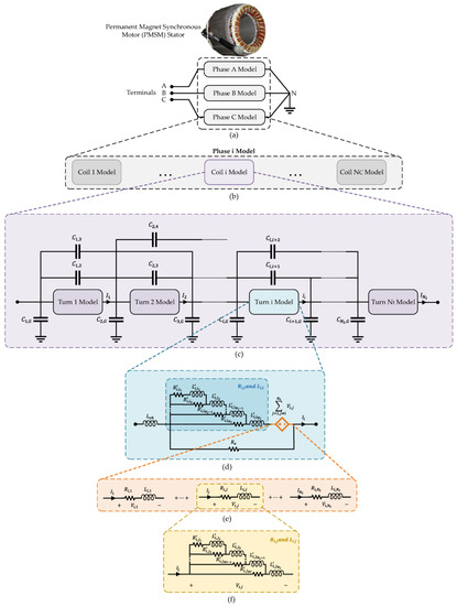
Figure 8.
The MCTL model of PMSM stator windings; (a) stator model; (b) phase model; (c) coil model; (d) turn model; (e) elements of controlled voltage source in turn model; (f) ladder circuits to model frequency-dependent resistances and inductances.
and are the self-resistance and inductance of turn ; is the current passing through the turn ; and are the mutual resistance and inductance between turn and ; and is the current passing through turn . Since all and are frequency dependent, the model should be a good representative of these elements in the intended frequency range. To capture the frequency-dependent behavior of resistances and inductances, ladder circuits [38] are employed, as shown in Figure 8d,f. Ladder circuits represent all and which are then be used to calculate and induced voltage due to the coupling between turns (, ≠ ). Also, to represent ∑, a controlled voltage source is considered in the turn model, as shown in Figure 8d, whose components (, , …) are computed using circuits shown in Figure 8e. For the sake of simplicity, however, induced voltages due to mutual coupling between different turns are not modeled using ladder circuits. Instead, mutual resistances and inductances are calculated at a specific frequency and are considered in the model.
In the turn model, represents the turn inductance in the overhang region and is considered 2.8 μH as calculated in [36]. Also, represents the core loss; if a resistance of 2 kΩ is assumed for each phase of the motor [39], is computed as:
in each turn model, where 8 is the number of coils in each phase connected in series (no parallel coils) and 11 is the number of turns in each coil.
4. Step-by-Step Procedure to Implement the MCTL Model of Stator Windings
In this section, the required steps to implement the model shown in Figure 8 are discussed in detail, and hints are provided on how exactly different elements in the model are computed. To develop the model, an FEM model of stator windings should be implemented to calculate parasitic elements of stator windings, including capacitances, inductances, and resistances. Essential parasitic elements of the stator windings are listed below [36]:
- Turn-to-core capacitances (to compute the capacitive coupling between turns and the core [ground]);
- Turn-to-turn capacitances (to compute the capacitive coupling between turns with one another);
- Self-resistance and -inductance of turns (to compute the frequency-dependent self-resistances and -inductances);
- Mutual resistances and inductances between a turn and all other turns (to compute the frequency-dependent mutual resistances and inductances between turns with one another).
After computing parasitic elements, since resistances and inductances are frequency dependent due to eddy current caused by skin effect at high frequencies, the frequency dependent behavior of resistances and inductances should be modeled. To this end, ladder circuits shown in Figure 8 are employed. As discussed in the following sections, a rational approximation of frequency domain responses by vector fitting is employed [40] to compute the corresponding values of elements in ladder circuits. Once elements of ladder circuits are calculated, the complete model of stator windings can be implemented so that the overvoltage phenomenon is studied in motor windings. In this article, the FEM model is simulated in COMSOL Multiphysics, elements of ladder circuits are computed using codes in MATLAB, and the final model is implemented and studied in EMTP-RV.
4.1. FEM Model Simulation in COMSOL Multiphysics
In this section, using the FEM model implemented in COMSOL Multiphysics, parasitic elements of stator windings are computed. The geometry of the stator is made using the information in Table 1 as shown in Figure 9a; for computation of parasitic elements, however, a single slot model suffices as shown in Figure 9b. There is no parallel coil, and each coil consists of 11 turns; each turn’s wire consists of 12 stranded wires which should be modeled accurately. Figure 10 shows how 11 turns are considered in the FEM model and Figure 11 depicts the mesh method utilized to calculate the required parasitic elements of the stator windings, which provides acceptable accuracy.
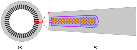
Figure 9.
FEM model geometry implemented in COMSOL Multiphysics; (a) complete 48-slot stator model; (b) one slot model.
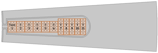
Figure 10.
The location of 11 turns in a slot.
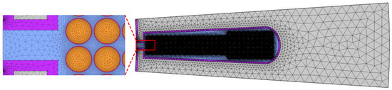
Figure 11.
The mesh method in COMSOL Multiphysics.
The skin effect in different turns was also considered and modeled. In this regard, Figure 12 shows the current density of turn 1 at a frequency of = 100 kHz when turn 1 is excited by 1 A and other turns are kept at 0 A.

Figure 12.
The influence of the skin effect on the current density of turn 1 (A/m2) when turn 1 is excited by 1 A and other turns are kept at 0 A at a frequency of 100 kHz.
4.1.1. Calculation of Turns’ Capacitances
To compute turns’ self and mutual capacitances, the electrostatics (es) solver is employed, where core boundaries are considered as ground; one turn (defined as terminal) is excited by a nonzero voltage (e.g., 1 V) and others are kept at 0 V. This procedure should then be repeated for all other turns but can be done sequentially by using the stationary source sweep in COMSOL Multiphysics to calculate the capacitance matrix. Note that entering a value for terminals is not needed when using the stationary source sweep to calculates the capacitance matrices. Also, if other values than 1 V are used, the software compensates for the values and the same capacitances are calculated. Finally, the mentioned procedure is how one should calculate capacitances in COMSOL; one cannot apply 1 V to one coil and keep others in 0 V in reality, since coils are not isolated, and all are connected together. The es solves Poisson’s equation as:
where is the electric displacement field, is the volume charge density, is the electric field, and is the scalar potential field. Using Equations (15) and (16), the Maxwell capacitance matrix and mutual capacitance matrix can be calculated. Note that these two matrices can be computed from each other as well. If the Maxwell capacitance matrix is defined as:
the mutual capacitance matrix can be calculated as:
Table 2 and Table 3 show the Maxwell capacitance matrix and the mutual capacitance matrix of different turns, respectively, resulted from the FEM simulation. Using these matrices, capacitances in the MCTL model are calculated. Since turns that are not close have little effect on each other, mutual capacitances are considered between turns and only if − as mentioned before.
Table 2.
The maxwell capacitance matrix (in F) resulting from FEM simulations.
Table 3.
The mutual capacitance matrix (in F) resulting from FEM simulations.
To calculate turn-to-core capacitance, it can be calculated as
A factor of 2 is considered to account for both conductors of a turn. Also, turn-to-turn capacitances between turn and can be calculated as
Similar to [36], turn-to-core capacitance in the overhang region is neglected due to the absence of the iron core in the overhang region. Instead, mutual capacitance in the overhang region per side is assumed to be equal to that for the slot region. Therefore, turn-to-turn capacitance can be updated as:
Indeed, a 3D FEM analysis of the 48-slot stator is needed to calculate the exact self and mutual capacitances in the overhang region. The mutual capacitance in the overhang region is assumed to be two times that in the slot region in [41]. Authors modified the assumption later in [36], considered the same mutual capacitance in the overhang region to the slot region, and validated the results using experiments. Therefore, the assumption in [36] is considered reliable in this article as well, and Equation (21) is considered reasonably precise until further studies.
4.1.2. Calculation of Turns’ Self and Mutual Inductances and Resistances
To calculate self and mutual inductances and resistances, the magnetic field (mf) solver in COMSOL Multiphysics is employed, where each turn is excited using a nonzero current (e.g., 1 A) while other turns are kept at 0 A; this procedure should be repeated for all turns. The mf solves Equations (22)–(25) as:
where is the magnetic field, is the electric current density, is the magnetic flux density, is the magnetic vector potential, is the conductivity of the medium, is the electric field, is the angular velocity, and is the electric displacement. The cut-off frequency of the considered PMSM is 1/~15 MHz; as a result, inductances and resistances are computed in seven different frequencies (50, 100, 1 k, 10 k, 100 k, 1 M, and 10 MHz) to properly capture the frequency-dependent behavior of inductances and resistances. After each field solution, inductances and resistances are computed using Equations (26) and (27) as in [12]:
where is the energy stored in the magnetic field (in joules [J]), is the ohmic loss (W), and is the peak value of the current (A) which is 1 A here. Turn 1 frequency-dependent inductances and resistances are presented in Table 4 and Table 5, respectively. In Appendix A and Appendix B, other turns’ self and mutual inductances and resistances resulting from the FEM simulation are also presented. Once and are calculated for all 11 turns, different elements in the model related to these parasitic parameters can be calculated. To account for the frequency dependency of and in the MCTL model, however, a rational approximation of frequency-dependent solutions is needed, as discussed in the next section.
Table 4.
Self and mutual inductances of turn 1 (in H) resulting from FEM simulations.
Table 5.
Self and mutual resistances of turn 1 (in Ω) resulting from FEM simulations.
4.2. Rational Approximation of the Frequency Domain Response
As discussed in previous sections, the parasitic inductances and resistances of motor windings are frequency dependent; it is essential to implement a model that accounts for this frequency dependency in the time domain. To this end, the rational approximation of frequency domain responses by vector fitting, which originally appeared in [40], is employed in this article. Using the so-called vector-fitting approach, a frequency-dependent function is approximated as:
where are residues and are poles and both are complex conjugate pairs, while and coefficients are essentially real. Using this definition, the problem is to determine , , , and so that the approximation is a good representative of the frequency-dependent function in the time domain. A comprehensive discussion of computing coefficients in Equation (28) falls beyond the scope of this article and readers may refer to [40] for more information; however, in the rest of this section, the applicability of the vector fitting is discussed for the purpose of this presented article.
Frequency-dependent self and mutual inductances and resistances ( and , = 1, 2, …, 11) are computed using the FEM simulations in 7 different frequencies (50–10 MHz). Ladder circuits are considered to represent the dependency on frequency. If the self-resistance and -inductance of turn 1 are considered as a frequency-dependent impedance (), it can be represented as below:
where and are the frequency-dependent self-resistance and -inductance of turn 1, respectively, and , where is a vector containing seven frequencies at which FEM simulations are done. Considering , is rewritten as:
where is the order of the ladder circuits. Once Equation (30) is solved, is found, and is then computed as [36]:
Once Equation (32) is solved, is found, and the new is computed as [36]:
Using the new and replacing with , the procedure in Equations (30)–(33) is repeated as long as . Finally, the procedure explained above for must be repeated for all obtained using and from FEM simulations, where (, number of turns).
The flowchart to calculate all elements in ladder circuits is shown in Figure 13. Using the flowchart, all elements in ladder circuits are calculated. The impedance of a ladder circuit ( should be a good representative of the FEM model simulations. The impedance of a ladder circuit is calculated as:
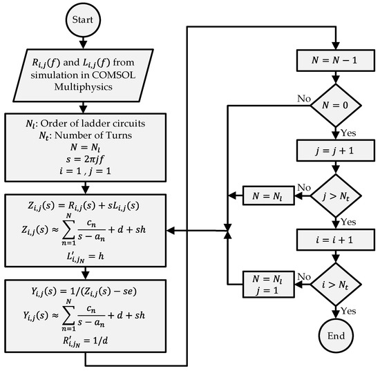
Figure 13.
The flowchart to calculate elements in ladder circuits using vector fitting.
is the number of layers in a ladder circuit and should be determined; while a higher results in a more precise representation, it also leads to a more complicated circuit and simulation burden. Figure 14 compares from the FEM model and calculated ladder circuits when = 4, 5, and 6. As shown, = 6 results in a ladder circuit properly representing the frequency dependent and . For all and , ladder circuits are considered as shown in Figure 15, and = 6 is selected. Table 6 presents elements of ladder circuits to account for the frequency-dependent self-resistances and -inductances of different turns ( and , = 1, 2, …, 11) calculated using vector fitting.
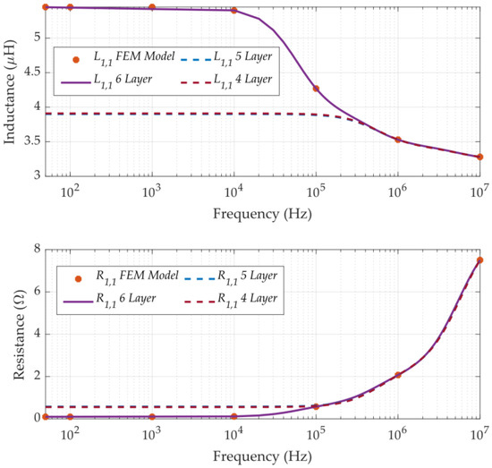
Figure 14.
Comparison of and resulting from FEM simulations and and resulting from ladder circuits with different layers calculated by vector fitting in MATLAB.
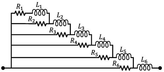
Figure 15.
Ladder circuits with six layers are implemented in the MCTL model of stator windings.
Table 6.
Elements of ladder circuits with six layers (R (Ω), L (H)) to represent the frequency-dependent self-resistances and -inductances of different turns in the MCTL model.
4.3. MCTL Model of Stator Windings in EMTP-RV
To study the overvoltage phenomenon in motor windings, the MCTL model of stator windings is implemented in EMTP-RV, a technically advanced analysis software for power system transients. Since all three phases and eight coils per phase are identical, it is appropriate to implement one coil model and copy the coil model to complete the model of stator windings. Also, to connect the motor model to the inverter model, a predefined cable model in EMTP-RV is used. Figure 16 shows one phase model in which eight identical coils are connected in series. To implement one coil model, 11 turns models are connected in series and implemented along with turn-to-core and turn-to-turn capacitances, as shown in Figure 17 and Figure 18.

Figure 16.
Phase model implemented in EMTP-RV; there are three identical phases and eight identical series coils per phase in the model.
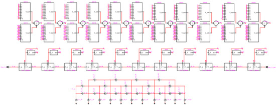
Figure 17.
One coil model implemented in EMTP-RV.

Figure 18.
One turn model implemented in EMTP-RV.
If ladder circuits are implemented to represent all and , (6 + 6 × 10) × 11 × 8 × 3 = 17,424 inductances are needed in the model to represent only . This number is apart from 1584 required inductances to represent inductances in the overhang region and the number of resistances, capacitances, controlled voltage and current sources, etc. Therefore, for the sake of simplicity and to keep the simulation burden as minimum as possible, ladder circuits are implemented only for representing self-resistances and -inductances in turns models. To account for and ( ≠ j), one inductance and one resistance are considered, which FEM simulations obtain their values at = 1 MHz. Once the FEM simulation is done, mutual resistances and inductances are calculated using Equations (26) and (27) and are employed in the model. Calculated and at = 1 MHz are found in Table 4 and Table 5 and Appendix A and Appendix B.
5. Simulation Results and Discussion
Once the MCTL model is completed, simulations are performed to study the overvoltage phenomenon in motor windings. In this section, different scenarios are simulated, and the results are shown and discussed. This section aims to represent the overvoltage in motor windings in different situations. It is widely accepted that the harshest situation occurs in turns closer to motor terminals. However, as shown in this section, the voltage in turns closer to the neutral can even exceed the voltage in turns closer to motor terminals when the neutral point is floating (it is not connected to the local ground [core]). This is due to the lack of a path for differential mode current to flow, which leads to an excessive voltage at turns closer to the neutral point. Therefore, the harshest situation occurs in turns closer to the neutral point and/or motor terminals depending on whether the neutral point is grounded or floating, whether a one-phase or three-phase excitation is assumed, etc. Also, the voltage distribution in different coils is non-uniform in all cases regardless of whether a single-phase or three-phase model is implemented and whether the neutral point is grounded or floating. All these factors must be carefully taken into consideration when designing the motor insulation system.
5.1. One-Phase Simulation with Grounded Neutral Point
In this case, a one-phase stator windings model is implemented and connected to the inverter model through a 5 m predefined lossy cable. The inverter is fed from a 560 V DC link and generates 100 kHz PWM voltages with = 20 ns. Note that a 5 m cable is used to ensure that a case close to the worst case considered in terms of the cable length. Figure 19 shows the coil-to-core (also ground in this case) voltages when one phase is excited by the inverter and the neutral point is also connected to the local ground, the stator core. Also, coil voltages are considered at the beginning of a coil, so the coil 1-to-core voltage represents the voltage at motor terminals as well. As shown, the voltage distribution is non-uniform, of which the harshest situation occurs in coil 1 where the voltage peak reaches 907 V, 62% higher than the DC link voltage. Also, the coil 1 voltage oscillates with a much higher frequency than other coils’ voltages. Finally, the slightest situation occurs in coil 8, the closet coil to the grounded neutral point. Also, as shown in Figure 20, if a three-phase model is implemented, the neutral point is grounded, and only one phase is excited, coil voltages of the excited phase are the same as shown in Figure 19.
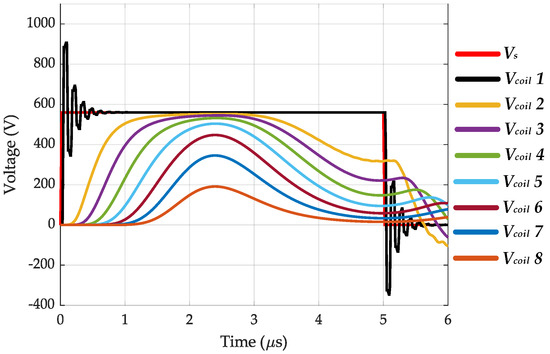
Figure 19.
Coil-to-core voltages of different coils when a single-phase model is implemented and is excited by a 560 V PWM voltage with = 20 ns and the neutral point is grounded.

Figure 20.
Three-phase model with grounded neutral point.
5.2. One-Phase Simulation with Floating Neutral Point
When the neutral point is floating, there is no path for currents to flow to the ground. As shown in Figure 21, this leads to voltage accumulation at turns closer to the neutral point. Consequently, the voltages of coils closer to the neutral point are greater than those closer to motor terminals. In this case, the voltage of coil 8 reaches 1063 V, which is 90% higher than the DC link voltage. The voltage distribution is also non-uniform, and the coil 1 voltage oscillates at an extremely higher frequency compared to voltages of other coils.
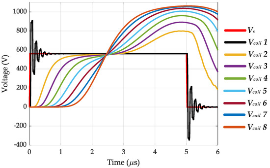
Figure 21.
Coil-to-core voltages of different coils when a single-phase model is implemented and is excited by a 560 V PWM voltage with = 20 ns and the neutral point is floating.
5.3. Three-Phase Simulation with Floating Neutral Point (One Phase Excitation)
In this case, the complete three-phase MCTL model of stator windings is considered, but only one phase is excited by PWM voltages, as shown in Figure 22. The voltages in different coils of the excited phase are shown in Figure 23. The voltages of coils closer to the neutral point are lower than those closer to motor terminals. The distribution of voltage is extremely non-uniform, and the coil 1 voltage oscillates at an extremely higher frequency compared to voltages of other coils. In this case, the harshest situation occurs at the turn closer to motor terminals and the voltage peak reaches 907 V, which is 62% higher than the DC link voltage.

Figure 22.
Three-phase model with floating neutral point.
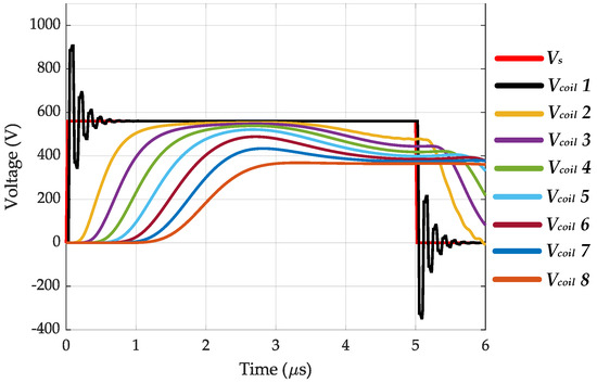
Figure 23.
Coil-to-core voltages of different coils when a three-phase model is implemented and only one phase is excited by a 560 V PWM voltage with = 20 ns and the neutral point is floating.
5.4. Model with Ladder Circuits vs. Model in a Fixed Frequency
In this section, coil voltages are compared when the MCTL model with ladder circuits is developed with the case of implementing a model in a fixed frequency without employing ladder circuits to account for frequency-dependent inductances and resistances. In this regard, the one-phase model in Section 5.1 and Section 5.2 is considered along with two fixed-frequency models in = 100 kHz (the main switching frequency) and = 1 MHz. Figure 24 and Figure 25 show coil voltages when the neutral point is grounded and floating, respectively; as shown, there is no difference in the voltage of the closest coil to motor terminals. Also, the difference in coil voltages is not too much when the neutral point is grounded, although the fixed-frequency model in the main switching frequency results in more similar voltage waveforms to the MCTL model with ladder circuits.
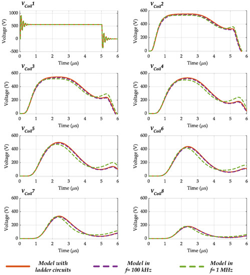
Figure 24.
The voltage in different coils when the MCTL model with ladder circuits is developed and fixed-frequency models are developed; the neutral point is grounded.
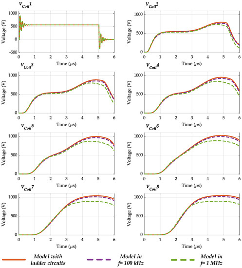
Figure 25.
The voltages in different coils when the MCTL model with ladder circuits is developed and fixed-frequency models are developed; the neutral point is floating.
However, when the neutral point is floating, the peak value of coil 8 voltage, for example, is obtained 1063 V in the model with ladder circuits, while it is ~1020 V in the model at = 100 kHz and ~896 V in the model at = 1 MHz. Therefore, one can conclude that modeling frequency-dependent inductances and resistances play a major role in precisely capturing the overvoltage phenomenon in motor windings, and it is especially important when the neutral point is floating. It is advisable to employ a model accounting for the frequency-dependent behavior of parasitic elements using ladder circuits, etc., to ensure capturing the transient overvoltages in motor windings precisely.
5.5. Discussion
In [36], ladder circuits were employed to model mutual inductances and resistances as well, and simulation results were validated using a prototype of the PMSM. Comparing the results in this section with those in [36], one can conclude that not only the developed model in this article is precise, but considering mutual inductances and resistances using ladder circuits in the model does not also play a major role in modeling the drive system. It is due to small values of mutual parasitic elements, and although ladder circuits are not employed in this article for mutual inductances and resistances, reasonable values are used in the model.
As shown in this section, when the motor windings are excited by a WBG-based inverter with high frequencies (100 kHz in this article) where the rise time of generated PWM voltages can be as low as 20 ns, the voltage distribution in different coils of the machine is non-uniform, where the voltage peak may reach to ~2 times that at inverter terminals. Also, the voltage of coils closer to the neutral point may even exceed the voltage of coils closer to motor terminals, depending on whether the neutral point is grounded or not. Finally, as shown in Figure 19, Figure 21 and Figure 23, the closest coil to motor terminals oscillates with a significantlyhigher frequency than other coils’ voltages. As a result, coils closer to the neutral point should also be carefully considered when designing the motor insulation system to avoid partial discharges and premature failures during the motor operation. One needs overvoltage amounts for insulation designs and coordination; precise calculations done in this article help to obtain accurate amounts of overvoltages on turns.
Figure 3, Figure 4, Figure 5, Figure 6 and Figure 7 in Section 2 show the transient overvoltages at motor terminals in extreme cases using a simplified circuit, while Figure 19, Figure 21 and Figure 23 show not only the overvoltage at motor terminals but also in all turns in motor windings using a realistic case study. Section 2 aims to show the impact of the cable length and rise time on transient overvoltages; also, while the overvoltage at motor terminals never reaches twice as much as that at the inverter terminals in simulations in Section 5, Section 2 shows the maximum possible overvoltage at motor terminals and the doubled voltage effect. In summary, simulations in Section 2 complete discussions in the following sections and aims to present the impact of the cable length and pulse rise time; a detailed analysis is done in the following sections using the developed model to properly evaluate the transient overvoltages at motor terminals and in all turns of the motor windings.
6. Conclusions
In this article, the repetitive overvoltage transients in WBG drive systems are discussed and analyzed in detail at motor terminals and in motor windings. To this end, an MCTL model of a PMSM stator winding adapted for EVs is implemented to assess the overvoltage phenomenon in motor windings. Also, a step-by-step procedure to arrive at the model is shown in detail. An FEM model of stator windings is simulated in COMSOL Multiphysics, considering skin and proximity effects; once the FEM simulation is completed, ladder circuits are designed to properly represent frequency-dependent elements resulting from FEM simulations. In this regard, rational approximation of frequency domain responses by vector fitting is employed by writing MATLAB codes to compute elements of ladder circuits. Finally, the MCTL model is implemented in EMTP-RV. As shown, the voltage at motor terminals may reach twice as much as that at inverter terminals, called the doubled voltage effect; also, the voltage distribution in motor windings is non-uniform, where the coil closer to motor terminals oscillates at an extremely high frequency compared to other coils. As shown by simulations, the transient peak voltage in motor windings occurs in turns closer to the motor terminals and/or turns closer to the neutral point. Determining the coil experiencing the harshest situation depends on several factors, such as how different phases are connected, whether the neutral point is grounded or floating, and how motor windings are excited. The overvoltage in turns closer to the neutral point can be harsher than in turns closer to the motor terminals. The model and studies presented in this article help us to better understand the overvoltage phenomenon in motor windings in order to pave the way for designing a proper insulation system for WBG drive systems.
Author Contributions
Conceptualization, M.G.; methodology, A.B. and M.G.; software, A.B.; validation, A.B. and M.G.; formal analysis, A.B. and M.G.; investigation, A.B. and M.G.; resources, A.B. and M.G.; data curation, A.B. and M.G.; writing—original draft preparation, A.B.; writing—review and editing, M.G.; visualization, A.B. and M.G.; supervision, M.G.; project administration, M.G.; funding acquisition, M.G. All authors have read and agreed to the published version of the manuscript.
Funding
This work was supported in part by the National Science Foundation (NSF) under Award 1942540.
Institutional Review Board Statement
Not applicable.
Informed Consent Statement
Not applicable.
Conflicts of Interest
The authors declare no conflict of interest.
Appendix A
In this appendix, the self and mutual inductances () of turns 2–11 (= 2, 3, …, 11, = 1, 2, …, 11) computed using FEM simulations in COMSOL Multiphysics are presented.
Table A1.
Self and mutual inductances of turn 2 (in H) resulting from FEM simulations.
Table A1.
Self and mutual inductances of turn 2 (in H) resulting from FEM simulations.
| T. no./Freq. | 1 | 2 | 3 | 4 | 5 | 6 | 7 | 8 | 9 | 10 | 11 |
|---|---|---|---|---|---|---|---|---|---|---|---|
| 50 Hz | 2.46 × 10⁻⁶ | 6.80 × 10⁻⁶ | 2.91 × 10⁻⁶ | 7.26 × 10⁻⁷ | 1.92 × 10⁻⁷ | 5.30 × 10⁻⁸ | 1.56 × 10⁻⁸ | 7.01 × 10⁻⁹ | 3.19 × 10⁻⁹ | 1.43 × 10⁻⁹ | 5.71 × 10⁻¹⁰ |
| 100 Hz | 2.46 × 10⁻⁶ | 6.80 × 10⁻⁶ | 2.91 × 10⁻⁶ | 7.26 × 10⁻⁷ | 1.92 × 10⁻⁷ | 5.30 × 10⁻⁸ | 1.56 × 10⁻⁸ | 7.01 × 10⁻⁹ | 3.19 × 10⁻⁹ | 1.43 × 10⁻⁹ | 5.71 × 10⁻¹⁰ |
| 1 kHz | 2.46 × 10⁻⁶ | 6.80 × 10⁻⁶ | 2.91 × 10⁻⁶ | 7.26 × 10⁻⁷ | 1.92 × 10⁻⁷ | 5.30 × 10⁻⁸ | 1.56 × 10⁻⁸ | 7.01 × 10⁻⁹ | 3.19 × 10⁻⁹ | 1.43 × 10⁻⁹ | 5.71 × 10⁻¹⁰ |
| 10 kHz | 2.44 × 10⁻⁶ | 6.73 × 10⁻⁶ | 2.89 × 10⁻⁶ | 7.27 × 10⁻⁷ | 1.93 × 10⁻⁷ | 5.34 × 10⁻⁸ | 1.57 × 10⁻⁸ | 7.05 × 10⁻⁹ | 3.20 × 10⁻⁹ | 1.44 × 10⁻⁹ | 5.69 × 10⁻¹⁰ |
| 100 kHz | 2.09 × 10⁻⁶ | 5.06 × 10⁻⁶ | 2.46 × 10⁻⁶ | 7.95 × 10⁻⁷ | 2.57 × 10⁻⁷ | 8.23 × 10⁻⁸ | 2.58 × 10⁻⁸ | 1.19 × 10⁻⁸ | 5.40 × 10⁻⁹ | 2.36 × 10⁻⁹ | 8.51 × 10⁻¹⁰ |
| 1 MHz | 1.92 × 10⁻⁶ | 3.92 × 10⁻⁶ | 2.17 × 10⁻⁶ | 8.98 × 10⁻⁷ | 3.78 × 10⁻⁷ | 1.58 × 10⁻⁷ | 6.25 × 10⁻⁸ | 3.50 × 10⁻⁸ | 1.98 × 10⁻⁸ | 1.12 × 10⁻⁸ | 6.12 × 10⁻⁹ |
| 10 MHz | 1.87 × 10⁻⁶ | 3.52 × 10⁻⁶ | 2.06 × 10⁻⁶ | 9.34 × 10⁻⁷ | 4.32 × 10⁻⁷ | 1.97 × 10⁻⁷ | 8.54 × 10⁻⁸ | 5.15 × 10⁻⁸ | 3.15 × 10⁻⁸ | 1.94 × 10⁻⁸ | 1.20 × 10⁻⁸ |
Table A2.
Self and mutual inductances of turn 3 (in H) resulting from FEM simulations.
Table A2.
Self and mutual inductances of turn 3 (in H) resulting from FEM simulations.
| T. no./Freq. | 1 | 2 | 3 | 4 | 5 | 6 | 7 | 8 | 9 | 10 | 11 |
|---|---|---|---|---|---|---|---|---|---|---|---|
| 50 Hz | 5.81 × 10⁻⁷ | 2.91 × 10⁻⁶ | 7.16 × 10⁻⁶ | 3.13 × 10⁻⁶ | 8.24 × 10⁻⁷ | 2.28 × 10⁻⁷ | 6.71 × 10⁻⁸ | 3.02 × 10⁻⁸ | 1.37 × 10⁻⁸ | 6.17 × 10⁻⁹ | 2.46 × 10⁻⁹ |
| 100 Hz | 5.81 × 10⁻⁷ | 2.91 × 10⁻⁶ | 7.16 × 10⁻⁶ | 3.13 × 10⁻⁶ | 8.24 × 10⁻⁷ | 2.28 × 10⁻⁷ | 6.71 × 10⁻⁸ | 3.02 × 10⁻⁸ | 1.37 × 10⁻⁸ | 6.17 × 10⁻⁹ | 2.46 × 10⁻⁹ |
| 1 kHz | 5.81 × 10⁻⁷ | 2.91 × 10⁻⁶ | 7.16 × 10⁻⁶ | 3.13 × 10⁻⁶ | 8.24 × 10⁻⁷ | 2.28 × 10⁻⁷ | 6.71 × 10⁻⁸ | 3.02 × 10⁻⁸ | 1.37 × 10⁻⁸ | 6.17 × 10⁻⁹ | 2.46 × 10⁻⁹ |
| 10 kHz | 5.81 × 10⁻⁷ | 2.89 × 10⁻⁶ | 7.09 × 10⁻⁶ | 3.11 × 10⁻⁶ | 8.25 × 10⁻⁷ | 2.29 × 10⁻⁷ | 6.75 × 10⁻⁸ | 3.04 × 10⁻⁸ | 1.38 × 10⁻⁸ | 6.20 × 10⁻⁹ | 2.46 × 10⁻⁹ |
| 100 kHz | 6.39 × 10⁻⁷ | 2.46 × 10⁻⁶ | 5.38 × 10⁻⁶ | 2.68 × 10⁻⁶ | 9.05 × 10⁻⁷ | 3.02 × 10⁻⁷ | 9.84 × 10⁻⁸ | 4.66 × 10⁻⁸ | 2.20 × 10⁻⁸ | 1.01 × 10⁻⁸ | 4.02 × 10⁻⁹ |
| 1 MHz | 7.62 × 10⁻⁷ | 2.17 × 10⁻⁶ | 4.16 × 10⁻⁶ | 2.36 × 10⁻⁶ | 1.00 × 10⁻⁶ | 4.22 × 10⁻⁷ | 1.69 × 10⁻⁷ | 9.53 × 10⁻⁸ | 5.43 × 10⁻⁸ | 3.09 × 10⁻⁸ | 1.71 × 10⁻⁸ |
| 10 MHz | 8.19 × 10⁻⁷ | 2.06 × 10⁻⁶ | 3.73 × 10⁻⁶ | 2.22 × 10⁻⁶ | 1.03 × 10⁻⁶ | 4.70 × 10⁻⁷ | 2.04 × 10⁻⁷ | 1.23 × 10⁻⁷ | 7.55 × 10⁻⁸ | 4.66 × 10⁻⁸ | 2.89 × 10⁻⁸ |
Table A3.
Self and mutual inductances of turn 4 (in H) resulting from FEM simulations.
Table A3.
Self and mutual inductances of turn 4 (in H) resulting from FEM simulations.
| T. no./Freq. | 1 | 2 | 3 | 4 | 5 | 6 | 7 | 8 | 9 | 10 | 11 |
|---|---|---|---|---|---|---|---|---|---|---|---|
| 50 Hz | 1.46 × 10⁻⁷ | 7.26 × 10⁻⁷ | 3.13 × 10⁻⁶ | 7.46 × 10⁻⁶ | 3.34 × 10⁻⁶ | 9.23 × 10⁻⁷ | 2.71 × 10⁻⁷ | 1.22 × 10⁻⁷ | 5.55 × 10⁻⁸ | 2.49 × 10⁻⁸ | 9.93 × 10⁻⁹ |
| 100 Hz | 1.46 × 10⁻⁷ | 7.26 × 10⁻⁷ | 3.13 × 10⁻⁶ | 7.46 × 10⁻⁶ | 3.34 × 10⁻⁶ | 9.23 × 10⁻⁷ | 2.71 × 10⁻⁷ | 1.22 × 10⁻⁷ | 5.55 × 10⁻⁸ | 2.49 × 10⁻⁸ | 9.93 × 10⁻⁹ |
| 1 kHz | 1.46 × 10⁻⁷ | 7.26 × 10⁻⁷ | 3.13 × 10⁻⁶ | 7.46 × 10⁻⁶ | 3.34 × 10⁻⁶ | 9.23 × 10⁻⁷ | 2.71 × 10⁻⁷ | 1.22 × 10⁻⁷ | 5.55 × 10⁻⁸ | 2.49 × 10⁻⁸ | 9.93 × 10⁻⁹ |
| 10 kHz | 1.46 × 10⁻⁷ | 7.27 × 10⁻⁷ | 3.11 × 10⁻⁶ | 7.39 × 10⁻⁶ | 3.32 × 10⁻⁶ | 9.24 × 10⁻⁷ | 2.72 × 10⁻⁷ | 1.23 × 10⁻⁷ | 5.58 × 10⁻⁸ | 2.51 × 10⁻⁸ | 9.98 × 10⁻⁹ |
| 100 kHz | 1.96 × 10⁻⁷ | 7.95 × 10⁻⁷ | 2.68 × 10⁻⁶ | 5.64 × 10⁻⁶ | 2.87 × 10⁻⁶ | 9.96 × 10⁻⁷ | 3.34 × 10⁻⁷ | 1.62 × 10⁻⁷ | 7.90 × 10⁻⁸ | 3.75 × 10⁻⁸ | 1.58 × 10⁻⁸ |
| 1 MHz | 3.11 × 10⁻⁷ | 8.98 × 10⁻⁷ | 2.36 × 10⁻⁶ | 4.37 × 10⁻⁶ | 2.51 × 10⁻⁶ | 1.06 × 10⁻⁶ | 4.29 × 10⁻⁷ | 2.44 × 10⁻⁷ | 1.40 × 10⁻⁷ | 8.02 × 10⁻⁸ | 4.49 × 10⁻⁸ |
| 10 MHz | 3.70 × 10⁻⁷ | 9.34 × 10⁻⁷ | 2.22 × 10⁻⁶ | 3.91 × 10⁻⁶ | 2.35 × 10⁻⁶ | 1.08 × 10⁻⁶ | 4.68 × 10⁻⁷ | 2.83 × 10⁻⁷ | 1.73 × 10⁻⁷ | 1.07 × 10⁻⁷ | 6.64 × 10⁻⁸ |
Table A4.
Self and mutual inductances of turn 5 (in H) resulting from FEM simulations.
Table A4.
Self and mutual inductances of turn 5 (in H) resulting from FEM simulations.
| T. no./Freq. | 1 | 2 | 3 | 4 | 5 | 6 | 7 | 8 | 9 | 10 | 11 |
|---|---|---|---|---|---|---|---|---|---|---|---|
| 50 Hz | 3.84 × 10⁻⁸ | 1.92 × 10⁻⁷ | 8.24 × 10⁻⁷ | 3.34 × 10⁻⁶ | 7.75 × 10⁻⁶ | 3.55 × 10⁻⁶ | 1.04 × 10⁻⁶ | 4.67 × 10⁻⁷ | 2.12 × 10⁻⁷ | 9.55 × 10⁻⁸ | 3.80 × 10⁻⁸ |
| 100 Hz | 3.84 × 10⁻⁸ | 1.92 × 10⁻⁷ | 8.24 × 10⁻⁷ | 3.34 × 10⁻⁶ | 7.75 × 10⁻⁶ | 3.55 × 10⁻⁶ | 1.04 × 10⁻⁶ | 4.67 × 10⁻⁷ | 2.12 × 10⁻⁷ | 9.55 × 10⁻⁸ | 3.80 × 10⁻⁸ |
| 1 kHz | 3.84 × 10⁻⁸ | 1.92 × 10⁻⁷ | 8.24 × 10⁻⁷ | 3.34 × 10⁻⁶ | 7.75 × 10⁻⁶ | 3.55 × 10⁻⁶ | 1.04 × 10⁻⁶ | 4.67 × 10⁻⁷ | 2.12 × 10⁻⁷ | 9.55 × 10⁻⁸ | 3.80 × 10⁻⁸ |
| 10 kHz | 3.86 × 10⁻⁸ | 1.93 × 10⁻⁷ | 8.25 × 10⁻⁷ | 3.32 × 10⁻⁶ | 7.67 × 10⁻⁶ | 3.53 × 10⁻⁶ | 1.04 × 10⁻⁶ | 4.67 × 10⁻⁷ | 2.13 × 10⁻⁷ | 9.59 × 10⁻⁸ | 3.82 × 10⁻⁸ |
| 100 kHz | 5.98 × 10⁻⁸ | 2.57 × 10⁻⁷ | 9.05 × 10⁻⁷ | 2.87 × 10⁻⁶ | 5.87 × 10⁻⁶ | 3.00 × 10⁻⁶ | 1.03 × 10⁻⁶ | 5.14 × 10⁻⁷ | 2.56 × 10⁻⁷ | 1.25 × 10⁻⁷ | 5.49 × 10⁻⁸ |
| 1 MHz | 1.29 × 10⁻⁷ | 3.78 × 10⁻⁷ | 1.00 × 10⁻⁶ | 2.51 × 10⁻⁶ | 4.52 × 10⁻⁶ | 2.55 × 10⁻⁶ | 1.04 × 10⁻⁶ | 5.92 × 10⁻⁷ | 3.42 × 10⁻⁷ | 1.97 × 10⁻⁷ | 1.12 × 10⁻⁷ |
| 10 MHz | 1.71 × 10⁻⁷ | 4.32 × 10⁻⁷ | 1.03 × 10⁻⁶ | 2.35 × 10⁻⁶ | 4.03 × 10⁻⁶ | 2.37 × 10⁻⁶ | 1.03 × 10⁻⁶ | 6.24 × 10⁻⁷ | 3.82 × 10⁻⁷ | 2.37 × 10⁻⁷ | 1.47 × 10⁻⁷ |
Table A5.
Self and mutual inductances of turn 6 (in H) resulting from FEM simulations.
Table A5.
Self and mutual inductances of turn 6 (in H) resulting from FEM simulations.
| T. no./Freq. | 1 | 2 | 3 | 4 | 5 | 6 | 7 | 8 | 9 | 10 | 11 |
|---|---|---|---|---|---|---|---|---|---|---|---|
| 50 Hz | 1.06 × 10⁻⁸ | 5.30 × 10⁻⁸ | 2.28 × 10⁻⁷ | 9.23 × 10⁻⁷ | 3.55 × 10⁻⁶ | 8.02 × 10⁻⁶ | 3.77 × 10⁻⁶ | 1.70 × 10⁻⁶ | 7.74 × 10⁻⁷ | 3.48 × 10⁻⁷ | 1.39 × 10⁻⁷ |
| 100 Hz | 1.06 × 10⁻⁸ | 5.30 × 10⁻⁸ | 2.28 × 10⁻⁷ | 9.23 × 10⁻⁷ | 3.55 × 10⁻⁶ | 8.02 × 10⁻⁶ | 3.77 × 10⁻⁶ | 1.70 × 10⁻⁶ | 7.74 × 10⁻⁷ | 3.48 × 10⁻⁷ | 1.39 × 10⁻⁷ |
| 1 kHz | 1.06 × 10⁻⁸ | 5.30 × 10⁻⁸ | 2.28 × 10⁻⁷ | 9.23 × 10⁻⁷ | 3.55 × 10⁻⁶ | 8.02 × 10⁻⁶ | 3.77 × 10⁻⁶ | 1.70 × 10⁻⁶ | 7.74 × 10⁻⁷ | 3.48 × 10⁻⁷ | 1.39 × 10⁻⁷ |
| 10 kHz | 1.07 × 10⁻⁸ | 5.34 × 10⁻⁸ | 2.29 × 10⁻⁷ | 9.24 × 10⁻⁷ | 3.53 × 10⁻⁶ | 7.94 × 10⁻⁶ | 3.74 × 10⁻⁶ | 1.69 × 10⁻⁶ | 7.72 × 10⁻⁷ | 3.48 × 10⁻⁷ | 1.39 × 10⁻⁷ |
| 100 kHz | 1.80 × 10⁻⁸ | 8.23 × 10⁻⁸ | 3.02 × 10⁻⁷ | 9.96 × 10⁻⁷ | 3.00 × 10⁻⁶ | 5.89 × 10⁻⁶ | 2.93 × 10⁻⁶ | 1.49 × 10⁻⁶ | 7.55 × 10⁻⁷ | 3.77 × 10⁻⁷ | 1.72 × 10⁻⁷ |
| 1 MHz | 5.31 × 10⁻⁸ | 1.58 × 10⁻⁷ | 4.22 × 10⁻⁷ | 1.06 × 10⁻⁶ | 2.55 × 10⁻⁶ | 4.42 × 10⁻⁶ | 2.38 × 10⁻⁶ | 1.37 × 10⁻⁶ | 7.95 × 10⁻⁷ | 4.62 × 10⁻⁷ | 2.63 × 10⁻⁷ |
| 10 MHz | 7.78 × 10⁻⁸ | 1.97 × 10⁻⁷ | 4.70 × 10⁻⁷ | 1.08 × 10⁻⁶ | 2.37 × 10⁻⁶ | 3.90 × 10⁻⁶ | 2.19 × 10⁻⁶ | 1.33 × 10⁻⁶ | 8.14 × 10⁻⁷ | 5.05 × 10⁻⁷ | 3.14 × 10⁻⁷ |
Table A6.
Self and mutual inductances of turn 7 (in H) resulting from FEM simulations.
Table A6.
Self and mutual inductances of turn 7 (in H) resulting from FEM simulations.
| T. no./Freq. | 1 | 2 | 3 | 4 | 5 | 6 | 7 | 8 | 9 | 10 | 11 |
|---|---|---|---|---|---|---|---|---|---|---|---|
| 50 Hz | 3.12 × 10⁻⁹ | 1.56 × 10⁻⁸ | 6.71 × 10⁻⁸ | 2.71 × 10⁻⁷ | 1.04 × 10⁻⁶ | 3.77 × 10⁻⁶ | 6.78 × 10⁻⁶ | 4.04 × 10⁻⁶ | 1.83 × 10⁻⁶ | 8.23 × 10⁻⁷ | 3.28 × 10⁻⁷ |
| 100 Hz | 3.12 × 10⁻⁹ | 1.56 × 10⁻⁸ | 6.71 × 10⁻⁸ | 2.71 × 10⁻⁷ | 1.04 × 10⁻⁶ | 3.77 × 10⁻⁶ | 6.78 × 10⁻⁶ | 4.04 × 10⁻⁶ | 1.83 × 10⁻⁶ | 8.23 × 10⁻⁷ | 3.28 × 10⁻⁷ |
| 1 kHz | 3.12 × 10⁻⁹ | 1.56 × 10⁻⁸ | 6.71 × 10⁻⁸ | 2.71 × 10⁻⁷ | 1.04 × 10⁻⁶ | 3.77 × 10⁻⁶ | 6.78 × 10⁻⁶ | 4.04 × 10⁻⁶ | 1.83 × 10⁻⁶ | 8.23 × 10⁻⁷ | 3.28 × 10⁻⁷ |
| 10 kHz | 3.13 × 10⁻⁹ | 1.57 × 10⁻⁸ | 6.75 × 10⁻⁸ | 2.72 × 10⁻⁷ | 1.04 × 10⁻⁶ | 3.74 × 10⁻⁶ | 6.70 × 10⁻⁶ | 3.99 × 10⁻⁶ | 1.82 × 10⁻⁶ | 8.19 × 10⁻⁷ | 3.27 × 10⁻⁷ |
| 100 kHz | 5.36 × 10⁻⁹ | 2.58 × 10⁻⁸ | 9.84 × 10⁻⁸ | 3.34 × 10⁻⁷ | 1.03 × 10⁻⁶ | 2.93 × 10⁻⁶ | 4.81 × 10⁻⁶ | 2.97 × 10⁻⁶ | 1.52 × 10⁻⁶ | 7.72 × 10⁻⁷ | 3.59 × 10⁻⁷ |
| 1 MHz | 2.08 × 10⁻⁸ | 6.25 × 10⁻⁸ | 1.69 × 10⁻⁷ | 4.29 × 10⁻⁷ | 1.04 × 10⁻⁶ | 2.38 × 10⁻⁶ | 3.64 × 10⁻⁶ | 2.41 × 10⁻⁶ | 1.40 × 10⁻⁶ | 8.17 × 10⁻⁷ | 4.68 × 10⁻⁷ |
| 10 MHz | 3.37 × 10⁻⁸ | 8.54 × 10⁻⁸ | 2.04 × 10⁻⁷ | 4.68 × 10⁻⁷ | 1.03 × 10⁻⁶ | 2.19 × 10⁻⁶ | 3.24 × 10⁻⁶ | 2.22 × 10⁻⁶ | 1.36 × 10⁻⁶ | 8.45 × 10⁻⁷ | 5.26 × 10⁻⁷ |
Table A7.
Self and mutual inductances of turn 8 (in H) resulting from FEM simulations.
Table A7.
Self and mutual inductances of turn 8 (in H) resulting from FEM simulations.
| T. no./Freq. | 1 | 2 | 3 | 4 | 5 | 6 | 7 | 8 | 9 | 10 | 11 |
|---|---|---|---|---|---|---|---|---|---|---|---|
| 50 Hz | 1.40 × 10⁻⁹ | 7.01 × 10⁻⁹ | 3.02 × 10⁻⁸ | 1.22 × 10⁻⁷ | 4.67 × 10⁻⁷ | 1.70 × 10⁻⁶ | 4.04 × 10⁻⁶ | 6.96 × 10⁻⁶ | 4.17 × 10⁻⁶ | 1.87 × 10⁻⁶ | 7.45 × 10⁻⁷ |
| 100 Hz | 1.40 × 10⁻⁹ | 7.01 × 10⁻⁹ | 3.02 × 10⁻⁸ | 1.22 × 10⁻⁷ | 4.67 × 10⁻⁷ | 1.70 × 10⁻⁶ | 4.04 × 10⁻⁶ | 6.96 × 10⁻⁶ | 4.17 × 10⁻⁶ | 1.87 × 10⁻⁶ | 7.45 × 10⁻⁷ |
| 1 kHz | 1.40 × 10⁻⁹ | 7.01 × 10⁻⁹ | 3.02 × 10⁻⁸ | 1.22 × 10⁻⁷ | 4.67 × 10⁻⁷ | 1.70 × 10⁻⁶ | 4.04 × 10⁻⁶ | 6.96 × 10⁻⁶ | 4.17 × 10⁻⁶ | 1.87 × 10⁻⁶ | 7.45 × 10⁻⁷ |
| 10 kHz | 1.41 × 10⁻⁹ | 7.05 × 10⁻⁹ | 3.04 × 10⁻⁸ | 1.23 × 10⁻⁷ | 4.67 × 10⁻⁷ | 1.69 × 10⁻⁶ | 3.99 × 10⁻⁶ | 6.87 × 10⁻⁶ | 4.12 × 10⁻⁶ | 1.86 × 10⁻⁶ | 7.42 × 10⁻⁷ |
| 100 kHz | 2.33 × 10⁻⁹ | 1.19 × 10⁻⁸ | 4.66 × 10⁻⁸ | 1.62 × 10⁻⁷ | 5.14 × 10⁻⁷ | 1.49 × 10⁻⁶ | 2.97 × 10⁻⁶ | 4.78 × 10⁻⁶ | 3.00 × 10⁻⁶ | 1.54 × 10⁻⁶ | 7.30 × 10⁻⁷ |
| 1 MHz | 1.16 × 10⁻⁸ | 3.50 × 10⁻⁸ | 9.53 × 10⁻⁸ | 2.44 × 10⁻⁷ | 5.92 × 10⁻⁷ | 1.37 × 10⁻⁶ | 2.41 × 10⁻⁶ | 3.55 × 10⁻⁶ | 2.40 × 10⁻⁶ | 1.40 × 10⁻⁶ | 8.10 × 10⁻⁷ |
| 10 MHz | 2.03 × 10⁻⁸ | 5.15 × 10⁻⁸ | 1.23 × 10⁻⁷ | 2.83 × 10⁻⁷ | 6.24 × 10⁻⁷ | 1.33 × 10⁻⁶ | 2.22 × 10⁻⁶ | 3.15 × 10⁻⁶ | 2.20 × 10⁻⁶ | 1.37 × 10⁻⁶ | 8.52 × 10⁻⁷ |
Table A8.
Self and mutual inductances of turn 9 (in H) resulting from FEM simulations.
Table A8.
Self and mutual inductances of turn 9 (in H) resulting from FEM simulations.
| T. no./Freq. | 1 | 2 | 3 | 4 | 5 | 6 | 7 | 8 | 9 | 10 | 11 |
|---|---|---|---|---|---|---|---|---|---|---|---|
| 50 Hz | 6.39 × 10⁻¹⁰ | 3.19 × 10⁻⁹ | 1.37 × 10⁻⁸ | 5.55 × 10⁻⁸ | 2.12 × 10⁻⁷ | 7.74 × 10⁻⁷ | 1.83 × 10⁻⁶ | 4.17 × 10⁻⁶ | 7.08 × 10⁻⁶ | 4.18 × 10⁻⁶ | 1.66 × 10⁻⁶ |
| 100 Hz | 6.39 × 10⁻¹⁰ | 3.19 × 10⁻⁹ | 1.37 × 10⁻⁸ | 5.55 × 10⁻⁸ | 2.12 × 10⁻⁷ | 7.74 × 10⁻⁷ | 1.83 × 10⁻⁶ | 4.17 × 10⁻⁶ | 7.08 × 10⁻⁶ | 4.18 × 10⁻⁶ | 1.66 × 10⁻⁶ |
| 1 kHz | 6.39 × 10⁻¹⁰ | 3.19 × 10⁻⁹ | 1.37 × 10⁻⁸ | 5.55 × 10⁻⁸ | 2.12 × 10⁻⁷ | 7.74 × 10⁻⁷ | 1.83 × 10⁻⁶ | 4.17 × 10⁻⁶ | 7.08 × 10⁻⁶ | 4.18 × 10⁻⁶ | 1.66 × 10⁻⁶ |
| 10 kHz | 6.37 × 10⁻¹⁰ | 3.20 × 10⁻⁹ | 1.38 × 10⁻⁸ | 5.58 × 10⁻⁸ | 2.13 × 10⁻⁷ | 7.72 × 10⁻⁷ | 1.82 × 10⁻⁶ | 4.12 × 10⁻⁶ | 6.99 × 10⁻⁶ | 4.13 × 10⁻⁶ | 1.65 × 10⁻⁶ |
| 100 kHz | 9.90 × 10⁻¹⁰ | 5.40 × 10⁻⁹ | 2.20 × 10⁻⁸ | 7.90 × 10⁻⁸ | 2.56 × 10⁻⁷ | 7.55 × 10⁻⁷ | 1.52 × 10⁻⁶ | 3.00 × 10⁻⁶ | 4.85 × 10⁻⁶ | 3.02 × 10⁻⁶ | 1.46 × 10⁻⁶ |
| 1 MHz | 6.47 × 10⁻⁹ | 1.98 × 10⁻⁸ | 5.43 × 10⁻⁸ | 1.40 × 10⁻⁷ | 3.42 × 10⁻⁷ | 7.95 × 10⁻⁷ | 1.40 × 10⁻⁶ | 2.40 × 10⁻⁶ | 3.60 × 10⁻⁶ | 2.44 × 10⁻⁶ | 1.41 × 10⁻⁶ |
| 10 MHz | 1.24 × 10⁻⁸ | 3.15 × 10⁻⁸ | 7.55 × 10⁻⁸ | 1.73 × 10⁻⁷ | 3.82 × 10⁻⁷ | 8.14 × 10⁻⁷ | 1.36 × 10⁻⁶ | 2.20 × 10⁻⁶ | 3.19 × 10⁻⁶ | 2.25 × 10⁻⁶ | 1.40 × 10⁻⁶ |
Table A9.
Self and mutual inductances of turn 10 (in H) resulting from FEM simulations.
Table A9.
Self and mutual inductances of turn 10 (in H) resulting from FEM simulations.
| T. no./Freq. | 1 | 2 | 3 | 4 | 5 | 6 | 7 | 8 | 9 | 10 | 11 |
|---|---|---|---|---|---|---|---|---|---|---|---|
| 50 Hz | 2.87 × 10⁻¹⁰ | 1.43 × 10⁻⁹ | 6.17 × 10⁻⁹ | 2.49 × 10⁻⁸ | 9.55 × 10⁻⁸ | 3.48 × 10⁻⁷ | 8.23 × 10⁻⁷ | 1.87 × 10⁻⁶ | 4.18 × 10⁻⁶ | 6.94 × 10⁻⁶ | 3.64 × 10⁻⁶ |
| 100 Hz | 2.87 × 10⁻¹⁰ | 1.43 × 10⁻⁹ | 6.17 × 10⁻⁹ | 2.49 × 10⁻⁸ | 9.55 × 10⁻⁸ | 3.48 × 10⁻⁷ | 8.23 × 10⁻⁷ | 1.87 × 10⁻⁶ | 4.18 × 10⁻⁶ | 6.94 × 10⁻⁶ | 3.64 × 10⁻⁶ |
| 1 kHz | 2.87 × 10⁻¹⁰ | 1.43 × 10⁻⁹ | 6.17 × 10⁻⁹ | 2.49 × 10⁻⁸ | 9.55 × 10⁻⁸ | 3.48 × 10⁻⁷ | 8.23 × 10⁻⁷ | 1.87 × 10⁻⁶ | 4.18 × 10⁻⁶ | 6.94 × 10⁻⁶ | 3.64 × 10⁻⁶ |
| 10 kHz | 2.85 × 10⁻¹⁰ | 1.44 × 10⁻⁹ | 6.20 × 10⁻⁹ | 2.51 × 10⁻⁸ | 9.59 × 10⁻⁸ | 3.48 × 10⁻⁷ | 8.19 × 10⁻⁷ | 1.86 × 10⁻⁶ | 4.13 × 10⁻⁶ | 6.85 × 10⁻⁶ | 3.60 × 10⁻⁶ |
| 100 kHz | 3.90 × 10⁻¹⁰ | 2.36 × 10⁻⁹ | 1.01 × 10⁻⁸ | 3.75 × 10⁻⁸ | 1.25 × 10⁻⁷ | 3.77 × 10⁻⁷ | 7.72 × 10⁻⁷ | 1.54 × 10⁻⁶ | 3.02 × 10⁻⁶ | 4.82 × 10⁻⁶ | 2.84 × 10⁻⁶ |
| 1 MHz | 3.61 × 10⁻⁹ | 1.12 × 10⁻⁸ | 3.09 × 10⁻⁸ | 8.02 × 10⁻⁸ | 1.97 × 10⁻⁷ | 4.62 × 10⁻⁷ | 8.17 × 10⁻⁷ | 1.40 × 10⁻⁶ | 2.44 × 10⁻⁶ | 3.64 × 10⁻⁶ | 2.44 × 10⁻⁶ |
| 10 MHz | 7.62 × 10⁻⁹ | 1.94 × 10⁻⁸ | 4.66 × 10⁻⁸ | 1.07 × 10⁻⁷ | 2.37 × 10⁻⁷ | 5.05 × 10⁻⁷ | 8.45 × 10⁻⁷ | 1.37 × 10⁻⁶ | 2.25 × 10⁻⁶ | 3.25 × 10⁻⁶ | 2.30 × 10⁻⁶ |
Table A10.
Self and mutual inductances of turn 11 (in H) resulting from FEM simulations.
Table A10.
Self and mutual inductances of turn 11 (in H) resulting from FEM simulations.
| T. no./Freq. | 1 | 2 | 3 | 4 | 5 | 6 | 7 | 8 | 9 | 10 | 11 |
|---|---|---|---|---|---|---|---|---|---|---|---|
| 50 Hz | 1.14 × 10⁻¹⁰ | 5.71 × 10⁻¹⁰ | 2.46 × 10⁻⁹ | 9.93 × 10⁻⁹ | 3.80 × 10⁻⁸ | 1.39 × 10⁻⁷ | 3.28 × 10⁻⁷ | 7.45 × 10⁻⁷ | 1.66 × 10⁻⁶ | 3.64 × 10⁻⁶ | 5.64 × 10⁻⁶ |
| 100 Hz | 1.14 × 10⁻¹⁰ | 5.71 × 10⁻¹⁰ | 2.46 × 10⁻⁹ | 9.93 × 10⁻⁹ | 3.80 × 10⁻⁸ | 1.39 × 10⁻⁷ | 3.28 × 10⁻⁷ | 7.45 × 10⁻⁷ | 1.66 × 10⁻⁶ | 3.64 × 10⁻⁶ | 5.64 × 10⁻⁶ |
| 1 kHz | 1.14 × 10⁻¹⁰ | 5.71 × 10⁻¹⁰ | 2.46 × 10⁻⁹ | 9.93 × 10⁻⁹ | 3.80 × 10⁻⁸ | 1.39 × 10⁻⁷ | 3.28 × 10⁻⁷ | 7.45 × 10⁻⁷ | 1.66 × 10⁻⁶ | 3.64 × 10⁻⁶ | 5.64 × 10⁻⁶ |
| 10 kHz | 1.13 × 10⁻¹⁰ | 5.69 × 10⁻¹⁰ | 2.46 × 10⁻⁹ | 9.98 × 10⁻⁹ | 3.82 × 10⁻⁸ | 1.39 × 10⁻⁷ | 3.27 × 10⁻⁷ | 7.42 × 10⁻⁷ | 1.65 × 10⁻⁶ | 3.60 × 10⁻⁶ | 5.59 × 10⁻⁶ |
| 100 kHz | 1.08 × 10⁻¹⁰ | 8.51 × 10⁻¹⁰ | 4.02 × 10⁻⁹ | 1.58 × 10⁻⁸ | 5.49 × 10⁻⁸ | 1.72 × 10⁻⁷ | 3.59 × 10⁻⁷ | 7.30 × 10⁻⁷ | 1.46 × 10⁻⁶ | 2.84 × 10⁻⁶ | 4.43 × 10⁻⁶ |
| 1 MHz | 1.94 × 10⁻⁹ | 6.12 × 10⁻⁹ | 1.71 × 10⁻⁸ | 4.49 × 10⁻⁸ | 1.12 × 10⁻⁷ | 2.63 × 10⁻⁷ | 4.68 × 10⁻⁷ | 8.10 × 10⁻⁷ | 1.41 × 10⁻⁶ | 2.44 × 10⁻⁶ | 3.59 × 10⁻⁶ |
| 10 MHz | 4.70 × 10⁻⁹ | 1.20 × 10⁻⁸ | 2.89 × 10⁻⁸ | 6.64 × 10⁻⁸ | 1.47 × 10⁻⁷ | 3.14 × 10⁻⁷ | 5.26 × 10⁻⁷ | 8.52 × 10⁻⁷ | 1.40 × 10⁻⁶ | 2.30 × 10⁻⁶ | 3.29 × 10⁻⁶ |
Appendix B
In this appendix, the self and mutual resistances () of turns 2–11 ( = 2, 3, …, 11, = 1, 2, …, 11) computed using FEM simulations in COMSOL Multiphysics are presented.
Table A11.
Self and mutual resistances of turn 2 (in Ω) resulting from FEM simulations.
Table A11.
Self and mutual resistances of turn 2 (in Ω) resulting from FEM simulations.
| T. no./Freq. | 1 | 2 | 3 | 4 | 5 | 6 | 7 | 8 | 9 | 10 | 11 |
|---|---|---|---|---|---|---|---|---|---|---|---|
| 50 Hz | 4.66 × 10⁻¹⁰ | 0.0962 | 5.52 × 10⁻¹⁰ | 6.20 × 10⁻¹¹ | 6.74 × 10⁻¹¹ | 3.15 × 10⁻¹¹ | 1.18 × 10⁻¹¹ | 6.09 × 10⁻¹² | 3.13 × 10⁻¹² | 1.58 × 10⁻¹² | 7.31 × 10⁻¹³ |
| 100 Hz | 9.32 × 10⁻¹⁰ | 0.0962 | 1.10 × 10⁻⁹ | 1.24 × 10⁻¹⁰ | 1.35 × 10⁻¹⁰ | 6.29 × 10⁻¹¹ | 2.37 × 10⁻¹¹ | 1.22 × 10⁻¹¹ | 6.25 × 10⁻¹² | 3.15 × 10⁻¹² | 1.46 × 10⁻¹² |
| 1 kHz | 9.32 × 10⁻⁹ | 0.0965 | 1.10 × 10⁻⁸ | 1.24 × 10⁻⁹ | 1.35 × 10⁻⁹ | 6.29 × 10⁻¹⁰ | 2.37 × 10⁻¹⁰ | 1.22 × 10⁻¹⁰ | 6.25 × 10⁻¹¹ | 3.15 × 10⁻¹¹ | 1.46 × 10⁻¹¹ |
| 10 kHz | 8.98 × 10⁻⁸ | 0.1219 | 1.07 × 10⁻⁷ | 1.25 × 10⁻⁸ | 1.34 × 10⁻⁸ | 6.28 × 10⁻⁹ | 2.37 × 10⁻⁹ | 1.22 × 10⁻⁹ | 6.27 × 10⁻¹⁰ | 3.17 × 10⁻¹⁰ | 1.47 × 10⁻¹⁰ |
| 100 kHz | 2.09 × 10⁻⁷ | 0.8225 | 2.90 × 10⁻⁷ | 7.97 × 10⁻⁸ | 8.14 × 10⁻⁸ | 4.38 × 10⁻⁸ | 1.86 × 10⁻⁸ | 1.06 × 10⁻⁸ | 5.99 × 10⁻⁹ | 3.30 × 10⁻⁹ | 1.72 × 10⁻⁹ |
| 1 MHz | 6.75 × 10⁻⁸ | 3.1409 | 1.28 × 10⁻⁷ | 4.22 × 10⁻⁸ | 5.56 × 10⁻⁸ | 3.74 × 10⁻⁸ | 2.00 × 10⁻⁸ | 1.36 × 10⁻⁸ | 9.10 × 10⁻⁹ | 6.06 × 10⁻⁹ | 4.04 × 10⁻⁹ |
| 10 MHz | 2.37 × 10⁻⁸ | 11.4956 | 5.10 × 10⁻⁸ | 1.62 × 10⁻⁸ | 2.44 × 10⁻⁸ | 1.80 × 10⁻⁸ | 1.07 × 10⁻⁸ | 7.75 × 10⁻⁹ | 5.57 × 10⁻⁹ | 4.00 × 10⁻⁹ | 2.92 × 10⁻⁹ |
Table A12.
Self and mutual resistances of turn 3 (in Ω) resulting from FEM simulations.
Table A12.
Self and mutual resistances of turn 3 (in Ω) resulting from FEM simulations.
| T. no./Freq. | 1 | 2 | 3 | 4 | 5 | 6 | 7 | 8 | 9 | 10 | 11 |
|---|---|---|---|---|---|---|---|---|---|---|---|
| 50 Hz | 5.25 × 10⁻¹¹ | 5.52 × 10⁻¹⁰ | 0.0962 | 5.63 × 10⁻¹⁰ | 7.33 × 10⁻¹¹ | 7.54 × 10⁻¹¹ | 3.33 × 10⁻¹¹ | 1.83 × 10⁻¹¹ | 9.85 × 10⁻¹² | 5.16 × 10⁻¹² | 2.50 × 10⁻¹² |
| 100 Hz | 1.05 × 10⁻¹⁰ | 1.10 × 10⁻⁹ | 0.0962 | 1.13 × 10⁻⁹ | 1.47 × 10⁻¹⁰ | 1.51 × 10⁻¹⁰ | 6.66 × 10⁻¹¹ | 3.66 × 10⁻¹¹ | 1.97 × 10⁻¹¹ | 1.03 × 10⁻¹¹ | 5.00 × 10⁻¹² |
| 1 kHz | 1.05 × 10⁻⁹ | 1.10 × 10⁻⁸ | 0.0965 | 1.13 × 10⁻⁸ | 1.47 × 10⁻⁹ | 1.51 × 10⁻⁹ | 6.66 × 10⁻¹⁰ | 3.66 × 10⁻¹⁰ | 1.97 × 10⁻¹⁰ | 1.03 × 10⁻¹⁰ | 5.00 × 10⁻¹¹ |
| 10 kHz | 1.07 × 10⁻⁸ | 1.07 × 10⁻⁷ | 0.1225 | 1.09 × 10⁻⁷ | 1.48 × 10⁻⁸ | 1.50 × 10⁻⁸ | 6.64 × 10⁻⁹ | 3.66 × 10⁻⁹ | 1.97 × 10⁻⁹ | 1.03 × 10⁻⁹ | 5.02 × 10⁻¹⁰ |
| 100 kHz | 8.02 × 10⁻⁸ | 2.90 × 10⁻⁷ | 0.8517 | 3.06 × 10⁻⁷ | 8.50 × 10⁻⁸ | 8.56 × 10⁻⁸ | 4.30 × 10⁻⁸ | 2.66 × 10⁻⁸ | 1.59 × 10⁻⁸ | 9.19 × 10⁻⁹ | 5.05 × 10⁻⁹ |
| 1 MHz | 5.79 × 10⁻⁸ | 1.28 × 10⁻⁷ | 3.3817 | 1.47 × 10⁻⁷ | 3.70 × 10⁻⁸ | 5.27 × 10⁻⁸ | 3.45 × 10⁻⁸ | 2.55 × 10⁻⁸ | 1.81 × 10⁻⁸ | 1.26 × 10⁻⁸ | 8.80 × 10⁻⁹ |
| 10 MHz | 2.60 × 10⁻⁸ | 5.10 × 10⁻⁸ | 12.6612 | 6.13 × 10⁻⁸ | 1.19 × 10⁻⁸ | 2.18 × 10⁻⁸ | 1.63 × 10⁻⁸ | 1.29 × 10⁻⁸ | 9.89 × 10⁻⁹ | 7.45 × 10⁻⁹ | 5.66 × 10⁻⁹ |
Table A13.
Self and mutual resistances of turn 4 (in Ω) resulting from FEM simulations.
Table A13.
Self and mutual resistances of turn 4 (in Ω) resulting from FEM simulations.
| T. no./Freq. | 1 | 2 | 3 | 4 | 5 | 6 | 7 | 8 | 9 | 10 | 11 |
|---|---|---|---|---|---|---|---|---|---|---|---|
| 50 Hz | 5.30 × 10⁻¹¹ | 6.20 × 10⁻¹¹ | 5.63 × 10⁻¹⁰ | 0.0962 | 5.82 × 10⁻¹⁰ | 6.53 × 10⁻¹¹ | 6.43 × 10⁻¹¹ | 4.24 × 10⁻¹¹ | 2.55 × 10⁻¹¹ | 1.44 × 10⁻¹¹ | 7.54 × 10⁻¹² |
| 100 Hz | 1.06 × 10⁻¹⁰ | 1.24 × 10⁻¹⁰ | 1.13 × 10⁻⁹ | 0.0962 | 1.16 × 10⁻⁹ | 1.31 × 10⁻¹⁰ | 1.29 × 10⁻¹⁰ | 8.48 × 10⁻¹¹ | 5.09 × 10⁻¹¹ | 2.88 × 10⁻¹¹ | 1.51 × 10⁻¹¹ |
| 1 kHz | 1.06 × 10⁻⁹ | 1.24 × 10⁻⁹ | 1.13 × 10⁻⁸ | 0.0965 | 1.16 × 10⁻⁸ | 1.31 × 10⁻⁹ | 1.29 × 10⁻⁹ | 8.48 × 10⁻¹⁰ | 5.09 × 10⁻¹⁰ | 2.88 × 10⁻¹⁰ | 1.51 × 10⁻¹⁰ |
| 10 kHz | 1.06 × 10⁻⁸ | 1.25 × 10⁻⁸ | 1.09 × 10⁻⁷ | 0.1230 | 1.13 × 10⁻⁷ | 1.31 × 10⁻⁸ | 1.28 × 10⁻⁸ | 8.44 × 10⁻⁹ | 5.08 × 10⁻⁹ | 2.88 × 10⁻⁹ | 1.51 × 10⁻⁹ |
| 100 kHz | 6.96 × 10⁻⁸ | 7.97 × 10⁻⁸ | 3.06 × 10⁻⁷ | 0.8761 | 3.31 × 10⁻⁷ | 6.84 × 10⁻⁸ | 6.95 × 10⁻⁸ | 5.22 × 10⁻⁸ | 3.50 × 10⁻⁸ | 2.20 × 10⁻⁸ | 1.31 × 10⁻⁸ |
| 1 MHz | 5.70 × 10⁻⁸ | 4.22 × 10⁻⁸ | 1.47 × 10⁻⁷ | 3.5515 | 1.68 × 10⁻⁷ | 2.21 × 10⁻⁸ | 4.21 × 10⁻⁸ | 3.87 × 10⁻⁸ | 3.10 × 10⁻⁸ | 2.34 × 10⁻⁸ | 1.75 × 10⁻⁸ |
| 10 MHz | 2.74 × 10⁻⁸ | 1.62 × 10⁻⁸ | 6.13 × 10⁻⁸ | 13.4588 | 7.13 × 10⁻⁸ | 4.94 × 10⁻⁹ | 1.76 × 10⁻⁸ | 1.78 × 10⁻⁸ | 1.54 × 10⁻⁸ | 1.25 × 10⁻⁸ | 1.02 × 10⁻⁸ |
Table A14.
Self and mutual resistances of turn 5 (in Ω) resulting from FEM simulations.
Table A14.
Self and mutual resistances of turn 5 (in Ω) resulting from FEM simulations.
| T. no./Freq. | 1 | 2 | 3 | 4 | 5 | 6 | 7 | 8 | 9 | 10 | 11 |
|---|---|---|---|---|---|---|---|---|---|---|---|
| 50 Hz | 2.42 × 10⁻¹¹ | 6.74 × 10⁻¹¹ | 7.33 × 10⁻¹¹ | 5.82 × 10⁻¹⁰ | 0.0962 | 6.66 × 10⁻¹⁰ | 1.71 × 10⁻¹¹ | 4.38 × 10⁻¹¹ | 4.36 × 10⁻¹¹ | 3.09 × 10⁻¹¹ | 1.92 × 10⁻¹¹ |
| 100 Hz | 4.84 × 10⁻¹¹ | 1.35 × 10⁻¹⁰ | 1.47 × 10⁻¹⁰ | 1.16 × 10⁻⁹ | 0.0962 | 1.33 × 10⁻⁹ | 3.41 × 10⁻¹¹ | 8.77 × 10⁻¹¹ | 8.72 × 10⁻¹¹ | 6.18 × 10⁻¹¹ | 3.84 × 10⁻¹¹ |
| 1 kHz | 4.84 × 10⁻¹⁰ | 1.35 × 10⁻⁹ | 1.47 × 10⁻⁹ | 1.16 × 10⁻⁸ | 0.0965 | 1.33 × 10⁻⁸ | 3.41 × 10⁻¹⁰ | 8.77 × 10⁻¹⁰ | 8.72 × 10⁻¹⁰ | 6.18 × 10⁻¹⁰ | 3.84 × 10⁻¹⁰ |
| 10 kHz | 4.84 × 10⁻⁹ | 1.34 × 10⁻⁸ | 1.48 × 10⁻⁸ | 1.13 × 10⁻⁷ | 0.1237 | 1.29 × 10⁻⁷ | 3.07 × 10⁻⁹ | 8.83 × 10⁻⁹ | 8.72 × 10⁻⁹ | 6.18 × 10⁻⁹ | 3.84 × 10⁻⁹ |
| 100 kHz | 3.66 × 10⁻⁸ | 8.14 × 10⁻⁸ | 8.50 × 10⁻⁸ | 3.31 × 10⁻⁷ | 0.9130 | 4.04 × 10⁻⁷ | 4.30 × 10⁻⁹ | 5.67 × 10⁻⁸ | 5.60 × 10⁻⁸ | 4.25 × 10⁻⁸ | 2.93 × 10⁻⁸ |
| 1 MHz | 3.72 × 10⁻⁸ | 5.56 × 10⁻⁸ | 3.70 × 10⁻⁸ | 1.68 × 10⁻⁷ | 3.7730 | 2.02 × 10⁻⁷ | 1.71 × 10⁻⁹ | 3.44 × 10⁻⁸ | 4.08 × 10⁻⁸ | 3.69 × 10⁻⁸ | 3.10 × 10⁻⁸ |
| 10 MHz | 1.94 × 10⁻⁸ | 2.44 × 10⁻⁸ | 1.19 × 10⁻⁸ | 7.13 × 10⁻⁸ | 14.3726 | 8.39 × 10⁻⁸ | 2.40 × 10⁻⁹ | 1.43 × 10⁻⁸ | 1.86 × 10⁻⁸ | 1.82 × 10⁻⁸ | 1.65 × 10⁻⁸ |
Table A15.
Self and mutual resistances of turn 6 (in Ω) resulting from FEM simulations.
Table A15.
Self and mutual resistances of turn 6 (in Ω) resulting from FEM simulations.
| T. no./Freq. | 1 | 2 | 3 | 4 | 5 | 6 | 7 | 8 | 9 | 10 | 11 |
|---|---|---|---|---|---|---|---|---|---|---|---|
| 50 Hz | 9.26 × 10⁻¹² | 3.15 × 10⁻¹¹ | 7.54 × 10⁻¹¹ | 6.53 × 10⁻¹¹ | 6.66 × 10⁻¹⁰ | 0.0962 | 1.01 × 10⁻⁹ | 2.71 × 10⁻¹⁰ | 3.73 × 10⁻¹¹ | 2.44 × 10⁻¹¹ | 3.49 × 10⁻¹¹ |
| 100 Hz | 1.85 × 10⁻¹¹ | 6.29 × 10⁻¹¹ | 1.51 × 10⁻¹⁰ | 1.31 × 10⁻¹⁰ | 1.33 × 10⁻⁹ | 0.0962 | 2.02 × 10⁻⁹ | 5.42 × 10⁻¹⁰ | 7.46 × 10⁻¹¹ | 4.88 × 10⁻¹¹ | 6.97 × 10⁻¹¹ |
| 1 kHz | 1.85 × 10⁻¹⁰ | 6.29 × 10⁻¹⁰ | 1.51 × 10⁻⁹ | 1.31 × 10⁻⁹ | 1.33 × 10⁻⁸ | 0.0965 | 2.02 × 10⁻⁸ | 5.42 × 10⁻⁹ | 7.46 × 10⁻¹⁰ | 4.88 × 10⁻¹⁰ | 6.97 × 10⁻¹⁰ |
| 10 kHz | 1.86 × 10⁻⁹ | 6.28 × 10⁻⁹ | 1.50 × 10⁻⁸ | 1.31 × 10⁻⁸ | 1.29 × 10⁻⁷ | 0.1272 | 1.96 × 10⁻⁷ | 5.22 × 10⁻⁸ | 6.85 × 10⁻⁹ | 5.06 × 10⁻⁹ | 7.00 × 10⁻⁹ |
| 100 kHz | 1.62 × 10⁻⁸ | 4.38 × 10⁻⁸ | 8.56 × 10⁻⁸ | 6.84 × 10⁻⁸ | 4.04 × 10⁻⁷ | 1.0116 | 5.63 × 10⁻⁷ | 1.27 × 10⁻⁷ | 1.54 × 10⁻⁸ | 5.05 × 10⁻⁸ | 5.21 × 10⁻⁸ |
| 1 MHz | 2.05 × 10⁻⁸ | 3.74 × 10⁻⁸ | 5.27 × 10⁻⁸ | 2.21 × 10⁻⁸ | 2.02 × 10⁻⁷ | 4.0446 | 2.32 × 10⁻⁷ | 5.15 × 10⁻⁸ | 1.84 × 10⁻⁸ | 4.13 × 10⁻⁸ | 4.68 × 10⁻⁸ |
| 10 MHz | 1.16 × 10⁻⁸ | 1.80 × 10⁻⁸ | 2.18 × 10⁻⁸ | 4.94 × 10⁻⁹ | 8.39 × 10⁻⁸ | 15.0903 | 8.87 × 10⁻⁸ | 2.03 × 10⁻⁸ | 8.48 × 10⁻⁹ | 1.95 × 10⁻⁸ | 2.32 × 10⁻⁸ |
Table A16.
Self and mutual resistances of turn 7 (in Ω) resulting from FEM simulations.
Table A16.
Self and mutual resistances of turn 7 (in Ω) resulting from FEM simulations.
| T. no./Freq. | 1 | 2 | 3 | 4 | 5 | 6 | 7 | 8 | 9 | 10 | 11 |
|---|---|---|---|---|---|---|---|---|---|---|---|
| 50 Hz | 3.24 × 10⁻¹² | 1.18 × 10⁻¹¹ | 3.33 × 10⁻¹¹ | 6.43 × 10⁻¹¹ | 1.71 × 10⁻¹¹ | 1.01 × 10⁻⁹ | 0.0962 | 1.32 × 10⁻⁹ | 3.90 × 10⁻¹⁰ | 7.76 × 10⁻¹¹ | 2.86 × 10⁻¹¹ |
| 100 Hz | 6.48 × 10⁻¹² | 2.37 × 10⁻¹¹ | 6.66 × 10⁻¹¹ | 1.29 × 10⁻¹⁰ | 3.41 × 10⁻¹¹ | 2.02 × 10⁻⁹ | 0.0962 | 2.63 × 10⁻⁹ | 7.79 × 10⁻¹⁰ | 1.55 × 10⁻¹⁰ | 5.73 × 10⁻¹¹ |
| 1 kHz | 6.48 × 10⁻¹¹ | 2.37 × 10⁻¹⁰ | 6.66 × 10⁻¹⁰ | 1.29 × 10⁻⁹ | 3.41 × 10⁻¹⁰ | 2.02 × 10⁻⁸ | 0.0965 | 2.63 × 10⁻⁸ | 7.79 × 10⁻⁹ | 1.55 × 10⁻⁹ | 5.73 × 10⁻¹⁰ |
| 10 kHz | 6.50 × 10⁻¹⁰ | 2.37 × 10⁻⁹ | 6.64 × 10⁻⁹ | 1.28 × 10⁻⁸ | 3.07 × 10⁻⁹ | 1.96 × 10⁻⁷ | 0.1252 | 2.54 × 10⁻⁷ | 7.49 × 10⁻⁸ | 1.46 × 10⁻⁸ | 5.91 × 10⁻⁹ |
| 100 kHz | 6.31 × 10⁻⁹ | 1.86 × 10⁻⁸ | 4.30 × 10⁻⁸ | 6.95 × 10⁻⁸ | 4.30 × 10⁻⁹ | 5.63 × 10⁻⁷ | 0.8824 | 6.44 × 10⁻⁷ | 1.64 × 10⁻⁷ | 4.48 × 10⁻⁹ | 6.06 × 10⁻⁸ |
| 1 MHz | 9.93 × 10⁻⁹ | 2.00 × 10⁻⁸ | 3.45 × 10⁻⁸ | 4.21 × 10⁻⁸ | 1.71 × 10⁻⁹ | 2.32 × 10⁻⁷ | 3.2337 | 2.37 × 10⁻⁷ | 5.22 × 10⁻⁸ | 2.36 × 10⁻⁸ | 5.44 × 10⁻⁸ |
| 10 MHz | 6.15 × 10⁻⁹ | 1.07 × 10⁻⁸ | 1.63 × 10⁻⁸ | 1.76 × 10⁻⁸ | 2.40 × 10⁻⁹ | 8.87 × 10⁻⁸ | 11.6947 | 8.74 × 10⁻⁸ | 1.84 × 10⁻⁸ | 1.24 × 10⁻⁸ | 2.62 × 10⁻⁸ |
Table A17.
Self and mutual resistances of turn 8 (in Ω) resulting from FEM simulations.
Table A17.
Self and mutual resistances of turn 8 (in Ω) resulting from FEM simulations.
| T. no./Freq. | 1 | 2 | 3 | 4 | 5 | 6 | 7 | 8 | 9 | 10 | 11 |
|---|---|---|---|---|---|---|---|---|---|---|---|
| 50 Hz | 1.61 × 10⁻¹² | 6.09 × 10⁻¹² | 1.83 × 10⁻¹¹ | 4.24 × 10⁻¹¹ | 4.38 × 10⁻¹¹ | 2.71 × 10⁻¹⁰ | 1.32 × 10⁻⁹ | 0.0962 | 1.44 × 10⁻⁹ | 4.23 × 10⁻¹⁰ | 3.29 × 10⁻¹¹ |
| 100 Hz | 3.22 × 10⁻¹² | 1.22 × 10⁻¹¹ | 3.66 × 10⁻¹¹ | 8.48 × 10⁻¹¹ | 8.77 × 10⁻¹¹ | 5.42 × 10⁻¹⁰ | 2.63 × 10⁻⁹ | 0.0962 | 2.89 × 10⁻⁹ | 8.46 × 10⁻¹⁰ | 6.58 × 10⁻¹¹ |
| 1 kHz | 3.22 × 10⁻¹¹ | 1.22 × 10⁻¹⁰ | 3.66 × 10⁻¹⁰ | 8.48 × 10⁻¹⁰ | 8.77 × 10⁻¹⁰ | 5.42 × 10⁻⁹ | 2.63 × 10⁻⁸ | 0.0965 | 2.89 × 10⁻⁸ | 8.45 × 10⁻⁹ | 6.57 × 10⁻¹⁰ |
| 10 kHz | 3.24 × 10⁻¹⁰ | 1.22 × 10⁻⁹ | 3.66 × 10⁻⁹ | 8.44 × 10⁻⁹ | 8.83 × 10⁻⁹ | 5.22 × 10⁻⁸ | 2.54 × 10⁻⁷ | 0.1288 | 2.79 × 10⁻⁷ | 8.13 × 10⁻⁸ | 5.89 × 10⁻⁹ |
| 100 kHz | 3.42 × 10⁻⁹ | 1.06 × 10⁻⁸ | 2.66 × 10⁻⁸ | 5.22 × 10⁻⁸ | 5.67 × 10⁻⁸ | 1.27 × 10⁻⁷ | 6.44 × 10⁻⁷ | 0.9421 | 7.00 × 10⁻⁷ | 1.79 × 10⁻⁷ | 3.32 × 10⁻⁸ |
| 1 MHz | 6.39 × 10⁻⁹ | 1.36 × 10⁻⁸ | 2.55 × 10⁻⁸ | 3.87 × 10⁻⁸ | 3.44 × 10⁻⁸ | 5.15 × 10⁻⁸ | 2.37 × 10⁻⁷ | 3.3390 | 2.52 × 10⁻⁷ | 5.40 × 10⁻⁸ | 3.92 × 10⁻⁸ |
| 10 MHz | 4.23 × 10⁻⁹ | 7.75 × 10⁻⁹ | 1.29 × 10⁻⁸ | 1.78 × 10⁻⁸ | 1.43 × 10⁻⁸ | 2.03 × 10⁻⁸ | 8.74 × 10⁻⁸ | 11.8503 | 9.08 × 10⁻⁸ | 1.78 × 10⁻⁸ | 1.89 × 10⁻⁸ |
Table A18.
Self and mutual resistances of turn 9 (in Ω) resulting from FEM simulations.
Table A18.
Self and mutual resistances of turn 9 (in Ω) resulting from FEM simulations.
| T. no./Freq. | 1 | 2 | 3 | 4 | 5 | 6 | 7 | 8 | 9 | 10 | 11 |
|---|---|---|---|---|---|---|---|---|---|---|---|
| 50 Hz | 8.05 × 10⁻¹³ | 3.13 × 10⁻¹² | 9.85 × 10⁻¹² | 2.55 × 10⁻¹¹ | 4.36 × 10⁻¹¹ | 3.73 × 10⁻¹¹ | 3.90 × 10⁻¹⁰ | 1.44 × 10⁻⁹ | 0.0962 | 1.42 × 10⁻⁹ | 2.59 × 10⁻¹⁰ |
| 100 Hz | 1.61 × 10⁻¹² | 6.25 × 10⁻¹² | 1.97 × 10⁻¹¹ | 5.09 × 10⁻¹¹ | 8.72 × 10⁻¹¹ | 7.46 × 10⁻¹¹ | 7.79 × 10⁻¹⁰ | 2.89 × 10⁻⁹ | 0.0962 | 2.84 × 10⁻⁹ | 5.18 × 10⁻¹⁰ |
| 1 kHz | 1.61 × 10⁻¹¹ | 6.25 × 10⁻¹¹ | 1.97 × 10⁻¹⁰ | 5.09 × 10⁻¹⁰ | 8.72 × 10⁻¹⁰ | 7.46 × 10⁻¹⁰ | 7.79 × 10⁻⁹ | 2.89 × 10⁻⁸ | 0.0965 | 2.84 × 10⁻⁸ | 5.18 × 10⁻⁹ |
| 10 kHz | 1.62 × 10⁻¹⁰ | 6.27 × 10⁻¹⁰ | 1.97 × 10⁻⁹ | 5.08 × 10⁻⁹ | 8.72 × 10⁻⁹ | 6.85 × 10⁻⁹ | 7.49 × 10⁻⁸ | 2.79 × 10⁻⁷ | 0.1295 | 2.74 × 10⁻⁷ | 4.96 × 10⁻⁸ |
| 100 kHz | 1.85 × 10⁻⁹ | 5.99 × 10⁻⁹ | 1.59 × 10⁻⁸ | 3.50 × 10⁻⁸ | 5.60 × 10⁻⁸ | 1.54 × 10⁻⁸ | 1.64 × 10⁻⁷ | 7.00 × 10⁻⁷ | 0.9631 | 6.88 × 10⁻⁷ | 9.02 × 10⁻⁸ |
| 1 MHz | 4.10 × 10⁻⁹ | 9.10 × 10⁻⁹ | 1.81 × 10⁻⁸ | 3.10 × 10⁻⁸ | 4.08 × 10⁻⁸ | 1.84 × 10⁻⁸ | 5.22 × 10⁻⁸ | 2.52 × 10⁻⁷ | 3.4064 | 2.45 × 10⁻⁷ | 1.88 × 10⁻⁸ |
| 10 MHz | 2.92 × 10⁻⁹ | 5.57 × 10⁻⁹ | 9.89 × 10⁻⁹ | 1.54 × 10⁻⁸ | 1.86 × 10⁻⁸ | 8.48 × 10⁻⁹ | 1.84 × 10⁻⁸ | 9.08 × 10⁻⁸ | 12.0282 | 8.77 × 10⁻⁸ | 5.20 × 10⁻⁹ |
Table A19.
Self and mutual resistances of turn 10 (in Ω) resulting from FEM simulations.
Table A19.
Self and mutual resistances of turn 10 (in Ω) resulting from FEM simulations.
| T. no./Freq. | 1 | 2 | 3 | 4 | 5 | 6 | 7 | 8 | 9 | 10 | 11 |
|---|---|---|---|---|---|---|---|---|---|---|---|
| 50 Hz | 3.96 × 10⁻¹³ | 1.58 × 10⁻¹² | 5.16 × 10⁻¹² | 1.44 × 10⁻¹¹ | 3.09 × 10⁻¹¹ | 2.44 × 10⁻¹¹ | 7.76 × 10⁻¹¹ | 4.23 × 10⁻¹⁰ | 1.42 × 10⁻⁹ | 0.0962 | 9.76 × 10⁻¹⁰ |
| 100 Hz | 7.92 × 10⁻¹³ | 3.15 × 10⁻¹² | 1.03 × 10⁻¹¹ | 2.88 × 10⁻¹¹ | 6.18 × 10⁻¹¹ | 4.88 × 10⁻¹¹ | 1.55 × 10⁻¹⁰ | 8.46 × 10⁻¹⁰ | 2.84 × 10⁻⁹ | 0.0962 | 1.95 × 10⁻⁹ |
| 1 kHz | 7.92 × 10⁻¹² | 3.15 × 10⁻¹¹ | 1.03 × 10⁻¹⁰ | 2.88 × 10⁻¹⁰ | 6.18 × 10⁻¹⁰ | 4.88 × 10⁻¹⁰ | 1.55 × 10⁻⁹ | 8.45 × 10⁻⁹ | 2.84 × 10⁻⁸ | 0.0965 | 1.95 × 10⁻⁸ |
| 10 kHz | 7.96 × 10⁻¹¹ | 3.17 × 10⁻¹⁰ | 1.03 × 10⁻⁹ | 2.88 × 10⁻⁹ | 6.18 × 10⁻⁹ | 5.06 × 10⁻⁹ | 1.46 × 10⁻⁸ | 8.13 × 10⁻⁸ | 2.74 × 10⁻⁷ | 0.1277 | 1.89 × 10⁻⁷ |
| 100 kHz | 9.80 × 10⁻¹⁰ | 3.30 × 10⁻⁹ | 9.19 × 10⁻⁹ | 2.20 × 10⁻⁸ | 4.25 × 10⁻⁸ | 5.05 × 10⁻⁸ | 4.48 × 10⁻⁹ | 1.79 × 10⁻⁷ | 6.88 × 10⁻⁷ | 0.9169 | 4.74 × 10⁻⁷ |
| 1 MHz | 2.64 × 10⁻⁹ | 6.06 × 10⁻⁹ | 1.26 × 10⁻⁸ | 2.34 × 10⁻⁸ | 3.69 × 10⁻⁸ | 4.13 × 10⁻⁸ | 2.36 × 10⁻⁸ | 5.40 × 10⁻⁸ | 2.45 × 10⁻⁷ | 3.2295 | 1.74 × 10⁻⁷ |
| 10 MHz | 2.02 × 10⁻⁹ | 4.00 × 10⁻⁹ | 7.45 × 10⁻⁹ | 1.25 × 10⁻⁸ | 1.82 × 10⁻⁸ | 1.95 × 10⁻⁸ | 1.24 × 10⁻⁸ | 1.78 × 10⁻⁸ | 8.77 × 10⁻⁸ | 11.4037 | 6.44 × 10⁻⁸ |
Table A20.
Self and mutual resistances of turn 11 (in Ω) resulting from FEM simulations.
Table A20.
Self and mutual resistances of turn 11 (in Ω) resulting from FEM simulations.
| T. no./Freq. | 1 | 2 | 3 | 4 | 5 | 6 | 7 | 8 | 9 | 10 | 11 |
|---|---|---|---|---|---|---|---|---|---|---|---|
| 50 Hz | 1.78 × 10⁻¹³ | 7.31 × 10⁻¹³ | 2.50 × 10⁻¹² | 7.54 × 10⁻¹² | 1.92 × 10⁻¹¹ | 3.49 × 10⁻¹¹ | 2.86 × 10⁻¹¹ | 3.29 × 10⁻¹¹ | 2.59 × 10⁻¹⁰ | 9.76 × 10⁻¹⁰ | 0.0962 |
| 100 Hz | 3.57 × 10⁻¹³ | 1.46 × 10⁻¹² | 5.00 × 10⁻¹² | 1.51 × 10⁻¹¹ | 3.84 × 10⁻¹¹ | 6.97 × 10⁻¹¹ | 5.73 × 10⁻¹¹ | 6.58 × 10⁻¹¹ | 5.18 × 10⁻¹⁰ | 1.95 × 10⁻⁹ | 0.0962 |
| 1 kHz | 3.57 × 10⁻¹² | 1.46 × 10⁻¹¹ | 5.00 × 10⁻¹¹ | 1.51 × 10⁻¹⁰ | 3.84 × 10⁻¹⁰ | 6.97 × 10⁻¹⁰ | 5.73 × 10⁻¹⁰ | 6.57 × 10⁻¹⁰ | 5.18 × 10⁻⁹ | 1.95 × 10⁻⁸ | 0.0964 |
| 10 kHz | 3.59 × 10⁻¹¹ | 1.47 × 10⁻¹⁰ | 5.02 × 10⁻¹⁰ | 1.51 × 10⁻⁹ | 3.84 × 10⁻⁹ | 7.00 × 10⁻⁹ | 5.91 × 10⁻⁹ | 5.89 × 10⁻⁹ | 4.96 × 10⁻⁸ | 1.89 × 10⁻⁷ | 0.1140 |
| 100 kHz | 4.86 × 10⁻¹⁰ | 1.72 × 10⁻⁹ | 5.05 × 10⁻⁹ | 1.31 × 10⁻⁸ | 2.93 × 10⁻⁸ | 5.21 × 10⁻⁸ | 6.06 × 10⁻⁸ | 3.32 × 10⁻⁸ | 9.02 × 10⁻⁸ | 4.74 × 10⁻⁷ | 0.6142 |
| 1 MHz | 1.70 × 10⁻⁹ | 4.04 × 10⁻⁹ | 8.80 × 10⁻⁹ | 1.75 × 10⁻⁸ | 3.10 × 10⁻⁸ | 4.68 × 10⁻⁸ | 5.44 × 10⁻⁸ | 3.92 × 10⁻⁸ | 1.88 × 10⁻⁸ | 1.74 × 10⁻⁷ | 2.3631 |
| 10 MHz | 1.43 × 10⁻⁹ | 2.92 × 10⁻⁹ | 5.66 × 10⁻⁹ | 1.02 × 10⁻⁸ | 1.65 × 10⁻⁸ | 2.32 × 10⁻⁸ | 2.62 × 10⁻⁸ | 1.89 × 10⁻⁸ | 5.20 × 10⁻⁹ | 6.44 × 10⁻⁸ | 8.7529 |
References
- Barzkar, A.; Ghassemi, M. Analysis of repetitive transient overvoltages in wide-bandgap drive systems. Electr. Power Syst. Res. 2022; submitted. [Google Scholar]
- Martínez-Tarifa, J.M.; Amaras-Duarte, H.; Sanz-Feito, J. Frequency-Domain Model for Calculation of Voltage Distribution through Random Wound Coils and Its Interaction with Stray Capacitances. IEEE Trans. Energy Convers. 2008, 23, 742–751. [Google Scholar] [CrossRef]
- Wright, M.; Yang, S.; McLeay, K. General theory of fast-fronted interturn voltage distribution in electrical machine windings. IEE Proc. B Electr. Power Appl. 1983, 130, 245–256. [Google Scholar] [CrossRef]
- Wright, M.; Yang, S.; McLeay, K. The influence of coil and surge parameters on transient interturn voltage distribution in stator windings. IEE Proc. B Electr. Power Appl. 1983, 130, 257–264. [Google Scholar] [CrossRef]
- McLaren, P.; Abdel-Rahman, M. Modeling of large AC motor coils for steep-fronted surge studies. IEEE Trans. Ind. Appl. 1988, 24, 422–426. [Google Scholar] [CrossRef]
- McLaren, P.; Oraee, H. Multiconductor transmission-line model for the line-end coil of large AC machines. IEE Proc. B Electr. Power Appl. 1985, 132, 149–156. [Google Scholar] [CrossRef]
- Guardado, J.; Cornick, K. A computer model for calculating steep-fronted surge distribution in machine windings. IEEE Trans. Energy Convers. 1989, 4, 95–101. [Google Scholar] [CrossRef]
- Paul, C.R. Analysis of Multiconductor Transmission Lines, 2nd ed.; John Wiley & Sons Inc.: Hoboken, NJ, USA, 2008. [Google Scholar]
- Lupo, G.; Petrarca, C.; Vitelli, M.; Tucci, V. Multiconductor transmission line analysis of steep-front surges in machine windings. IEEE Trans. Dielectr. Electr. Insul. 2002, 9, 467–478. [Google Scholar] [CrossRef]
- Melfi, M.; Sung, A.; Bell, S.; Skibinski, G. Effect of surge voltage risetime on the insulation of low-voltage machines fed by PWM converters. IEEE Trans. Ind. Appl. 1998, 34, 766–775. [Google Scholar] [CrossRef]
- Bonnett, A. Analysis of the impact of pulse-width modulated inverter voltage waveforms on AC induction motors. IEEE Trans. Ind. Appl. 1996, 32, 386–392. [Google Scholar] [CrossRef]
- Suresh, G.; Toliyat, H.; Rendusara, D.; Enjeti, P. Predicting the transient effects of PWM voltage waveform on the stator windings of random wound induction motors. IEEE Trans. Power Electron. 1999, 14, 23–30. [Google Scholar] [CrossRef]
- Mirafzal, B.; Skibinski, G.L.; Tallam, R.M.; Schlegel, D.W.; Lukaszewski, R.A. Universal Induction Motor Model with Low-to-High Frequency-Response Characteristics. IEEE Trans. Ind. Appl. 2007, 43, 1233–1246. [Google Scholar] [CrossRef]
- Hussain, M.K.; Gomez, P.; Espino-Cortes, F.P. Electromagnetic transient modeling of form-wound stator coils with stress grading system under PWM excitation. Electr. Power Syst. Res. 2021, 195, 107166. [Google Scholar] [CrossRef]
- Nuricumbo-Guillén, R.; Cortés, F.P.E.; Gómez, P.; Martínez, C.T. Computation of Transient Profiles along Nonuniform Transmission Lines Including Time-Varying and Nonlinear Elements Using the Numerical Laplace Transform. Energies 2019, 12, 3227. [Google Scholar] [CrossRef] [Green Version]
- Diab, M.; Zhou, W.; Emersic, C.; Yuan, X.; Cotton, I. Impact of PWM voltage waveforms on magnet wire insulation partial discharge in SiC-based motor drives. IEEE Access 2021, 9, 156599–156612. [Google Scholar] [CrossRef]
- Ju, X.; Cheng, Y.; Yang, M.; Cui, S.; Sun, A.; Liu, X.; He, M.H. Voltage Stress Calculation and Measurement for Hairpin Winding of EV Traction Machines Driven by SiC MOSFET. IEEE Trans. Ind. Electron. 2021, 69, 8803–8814. [Google Scholar] [CrossRef]
- Taghia, B.; Cougo, B.; Piquet, H.; Malec, D.; Belinger, A.; Carayon, J.-P. Overvoltage at motor terminals in SiC-based PWM drives. Math. Comput. Simul. 2019, 158, 264–280. [Google Scholar] [CrossRef] [Green Version]
- Barzkar, A.; Ghassemi, M. Components of Electrical Power Systems in More and All-Electric Aircraft: A Review. IEEE Trans. Transp. Electrif. 2022, 1. [Google Scholar] [CrossRef]
- Ghassemi, M.; Barzkar, A.; Saghafi, M. All-Electric NASA N3-X Aircraft Electric Power Systems. IEEE Trans. Transp. Electrif. 2022, 1. [Google Scholar] [CrossRef]
- Barzkar, A.; Ghassemi, M. Electric power systems in more and all electric aircraft: A review. IEEE Access 2020, 8, 169314–169332. [Google Scholar] [CrossRef]
- Ardeshiri, A.; Lotfi, A.; Behkam, R.; Moradzadeh, A.; Barzkar, A. Introduction and literature review of power system challenges and issues. In Application of Machine Learning and Deep Learning Methods to Power System Problems; Springer: Cham, Switzerland, 2021. [Google Scholar]
- Barzkar, A.; Tahami, F.; Barzkar, A. A hybrid control approach for LLC resonant converter. In Proceedings of the 2021 12th Power Electronics, Drive Systems, and Technologies Conference (PEDSTC 2021), Tabriz, Iran, 2–4 February 2021; pp. 1–6. [Google Scholar]
- Millan, J.; Godignon, P.; Perpina, X.; Perez-Tomas, A.; Rebollo, J. A Survey of Wide Bandgap Power Semiconductor Devices. IEEE Trans. Power Electron. 2013, 29, 2155–2163. [Google Scholar] [CrossRef]
- Wang, F.F.; Zhang, Z. Overview of Silicon Carbide Technology: Device, Converter, System, and Application. CPSS Trans. Power Electron. Appl. 2016, 1, 13–32. [Google Scholar] [CrossRef]
- She, X.; Huang, A.Q.; Lucia, O.; Ozpineci, B. Review of Silicon Carbide Power Devices and Their Applications. IEEE Trans. Ind. Electron. 2017, 64, 8193–8205. [Google Scholar] [CrossRef]
- Hussain, M.K.; Gomez, P. Optimized dielectric design of stator windings from medium voltage induction machines fed by fast front pulses. IEEE Trans. Dielectr. Electr. Insul. 2017, 24, 837–846. [Google Scholar] [CrossRef]
- Ghassemi, M. High power density technologies for large generators and motors for marine applications with focus on electrical insulation challenges. High Volt. 2020, 5, 7–14. [Google Scholar] [CrossRef]
- Ghassemi, M. Accelerated insulation aging due to fast, repetitive voltages: A review identifying challenges and future research needs. IEEE Trans. Dielectr. Electr. Insul. 2019, 26, 1558–1568. [Google Scholar] [CrossRef]
- Bewley, L.V. Traveling Waves on Transmission Systems. Cond. Affect. Success Main Line Electrif. 1931, 50, 532–550. [Google Scholar] [CrossRef]
- Madonna, V.; Giangrande, P.; Zhao, W.; Zhang, H.; Gerada, C.; Galea, M. On the Design of Partial Discharge-Free Low Voltage Electrical Machines. In Proceedings of the 2019 IEEE International Electric Machines & Drives Conference (IEMDC), San Deigo, CA, USA, 12–15 May 2019. [Google Scholar]
- Xu, Y.; Yuan, X.; Ye, F.; Wang, Z.; Zhang, Y.; Diab, M.; Zhou, W. Impact of High Switching Speed and High Switching Frequency of Wide-Bandgap Motor Drives on Electric Machines. IEEE Access 2021, 9, 82866–82880. [Google Scholar] [CrossRef]
- Hussain, M.; Gomez, P. Optimal filter tuning to minimize the transient overvoltages on machine windings fed by PWM inverters. In Proceedings of the 49th North American Power Symposium (NAPS), Morgantown, WV, USA, 17–19 September 2017. [Google Scholar]
- He, J.; Li, C.; Jassal, A.; Thiagarajan, N.; Zhang, Y.; Prabhakaran, S.; Feliz, C.; Graham, J.; Kang, X. Multi-domain design optimization of dv/dt filter for SiC-based three-phase inverters in high-frequency motor-drive applications. IEEE Trans. Ind. Appl. 2019, 55, 5214–5222. [Google Scholar]
- Diab, M.S.; Zhou, W.; Yuan, X. Evaluation of topologies and active control methods for overvoltage mitigation in SiC-based motor drives. In Proceedings of the IEEE Energy Conversion Congress and Exposition (ECCE), Vancouver, BC, Canada, 10–14 October 2021. [Google Scholar]
- Sundeep, S.; Wang, J.; Griffo, A. Holistic Modeling of High-Frequency Behavior of Inverter-Fed Machine Winding, Considering Mutual Couplings in Time Domain. IEEE Trans. Ind. Appl. 2021, 57, 6044–6057. [Google Scholar] [CrossRef]
- Olszewski, M. Evaluation of the 2010 Toyota Prius Hybrid Synergy Drive System. 2011. Available online: https://info.ornl.gov/sites/publications/files/Pub26762.pdf (accessed on 2 May 2022).
- De Paula, H.; de Andrade, D.A.; Chaves, M.L.R.; Domingos, J.L.; de Freitas, M.A.A. Methodology for Cable Modeling and Simulation for High-Frequency Phenomena Studies in PWM Motor Drives. IEEE Trans. Power Electron. 2008, 23, 744–752. [Google Scholar] [CrossRef]
- IEC/TS 61800-8; Adjustable Speed Electrical Power Drive Systems—Part 8: Specification of Voltage on the Power Interface. International Electrotechnical Commission: Geneva, Switzerland, 2010.
- Gustavsen, B.; Semlyen, A. Rational approximation of frequency domain responses by vector fitting. IEEE Trans. Power Deliv. 1999, 14, 1052–1061. [Google Scholar] [CrossRef] [Green Version]
- Sundeep, S.; Wang, J.; Griffo, A. Prediction of Transient Voltage Distribution in Inverter-fed Stator Winding, Considering Mutual Couplings in Time Domain. In Proceedings of the IEEE Energy Conversion Congress and Exposition (ECCE 2020), Detroit, MI, USA, 11–15 October 2020. [Google Scholar]
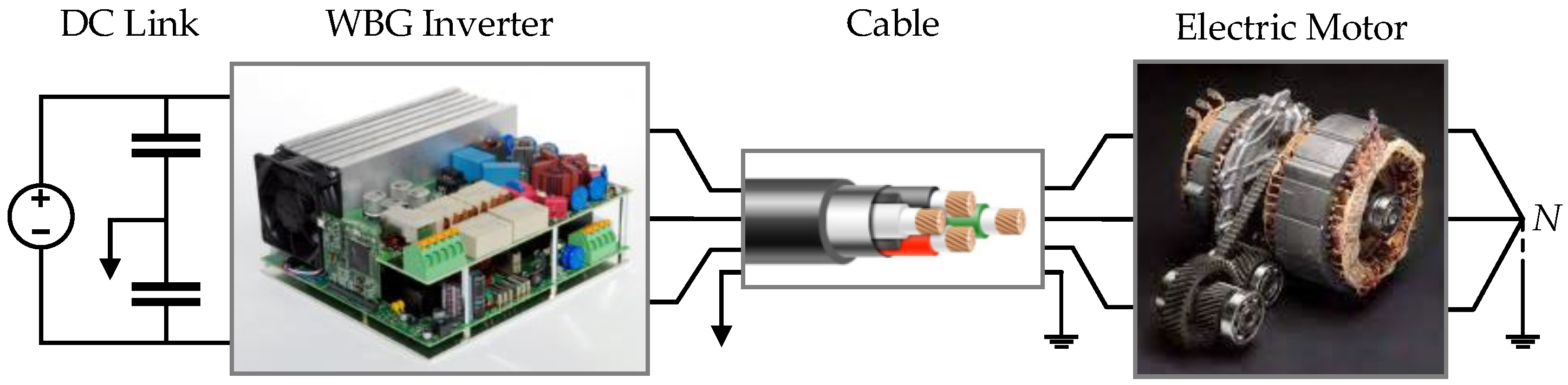
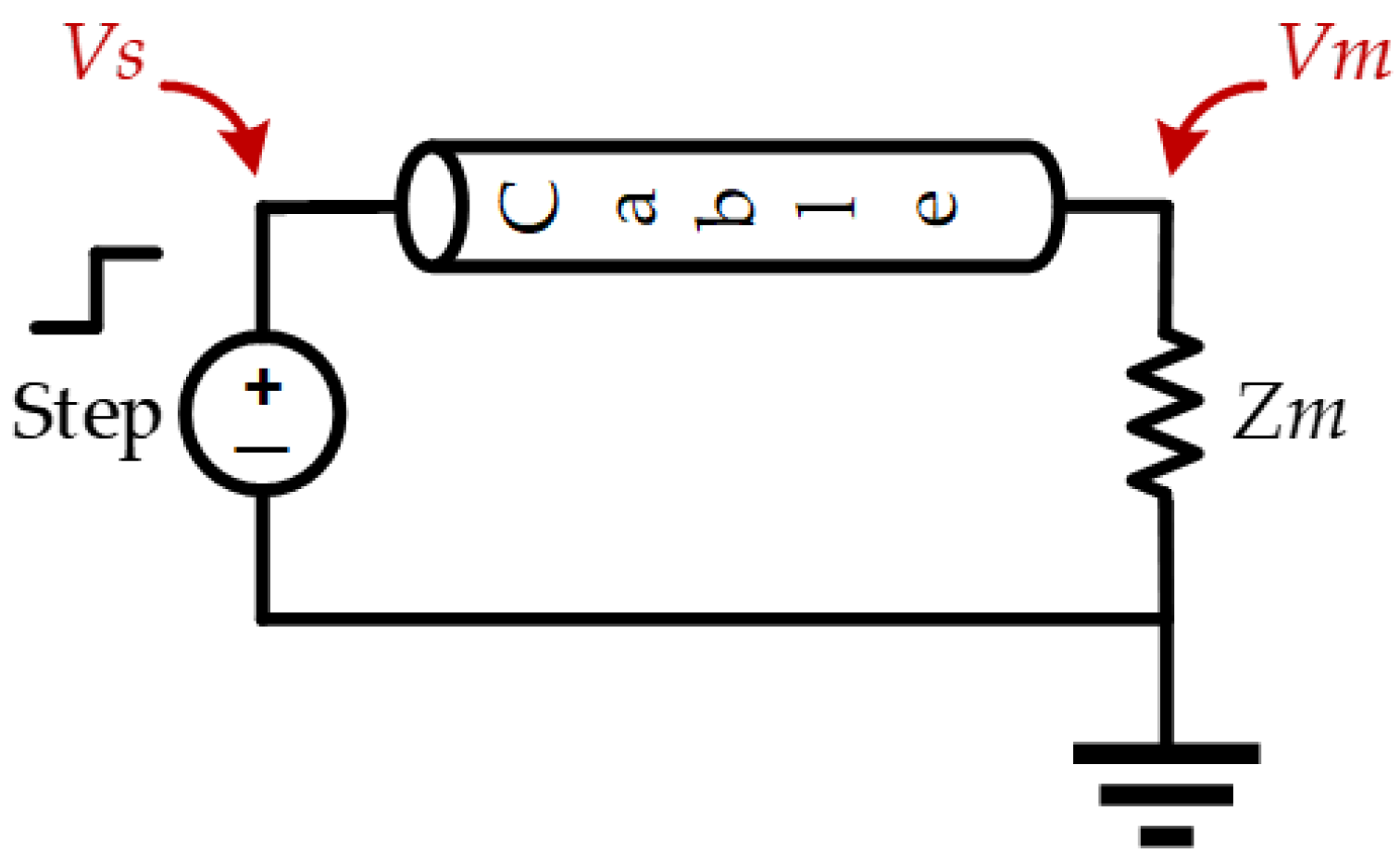

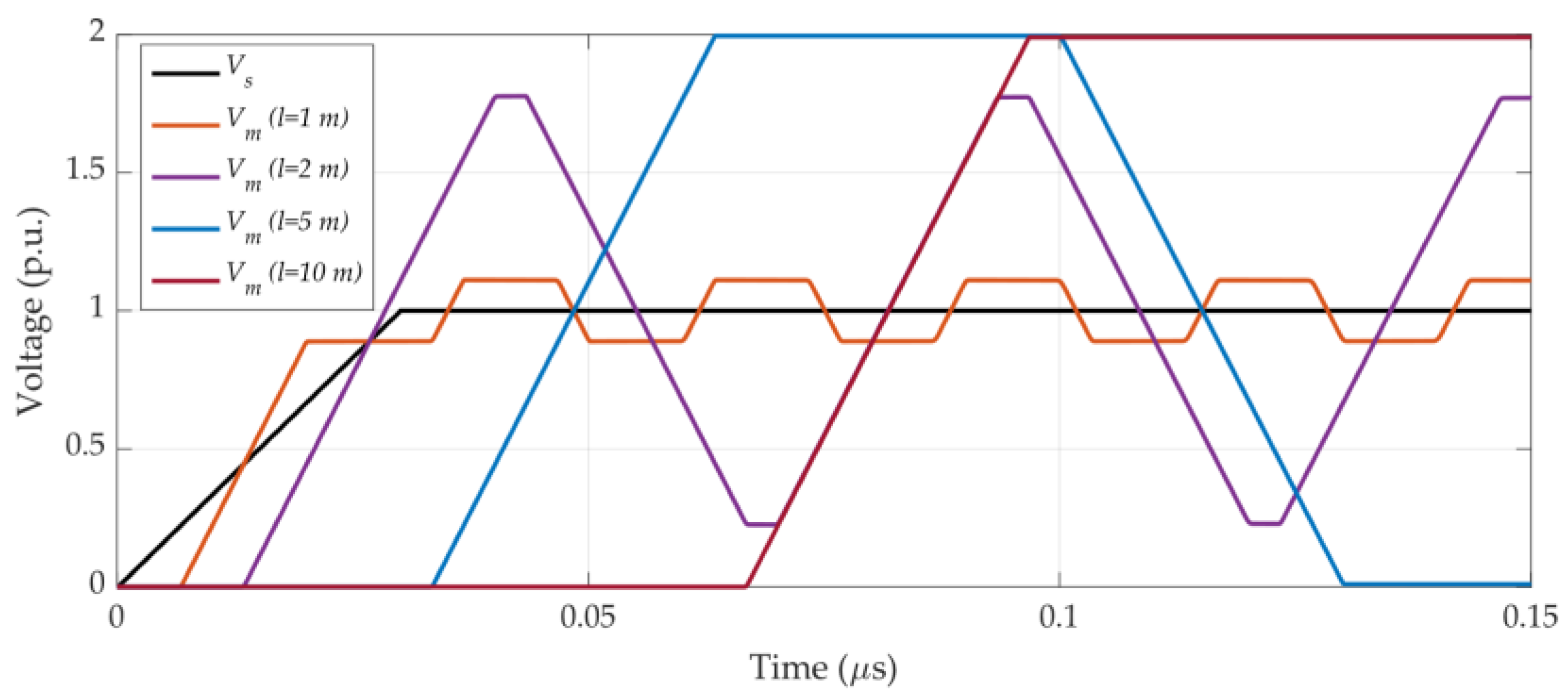
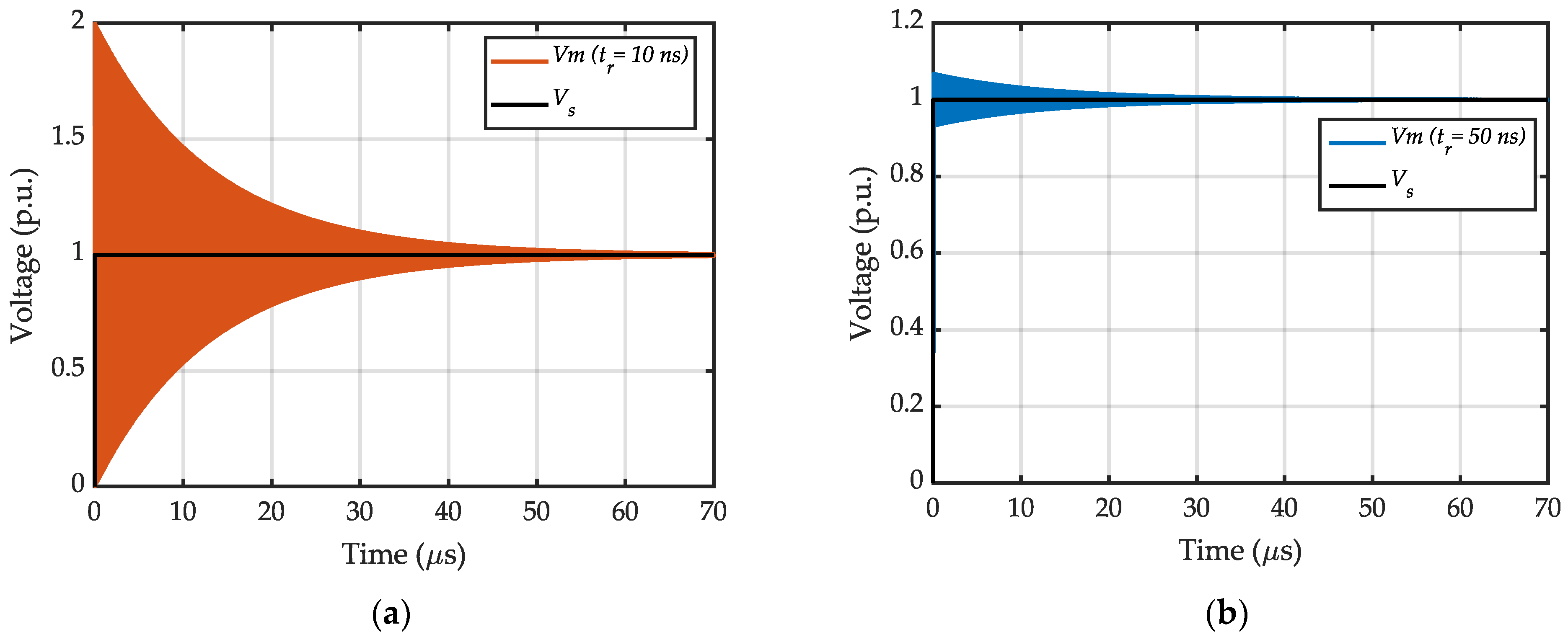


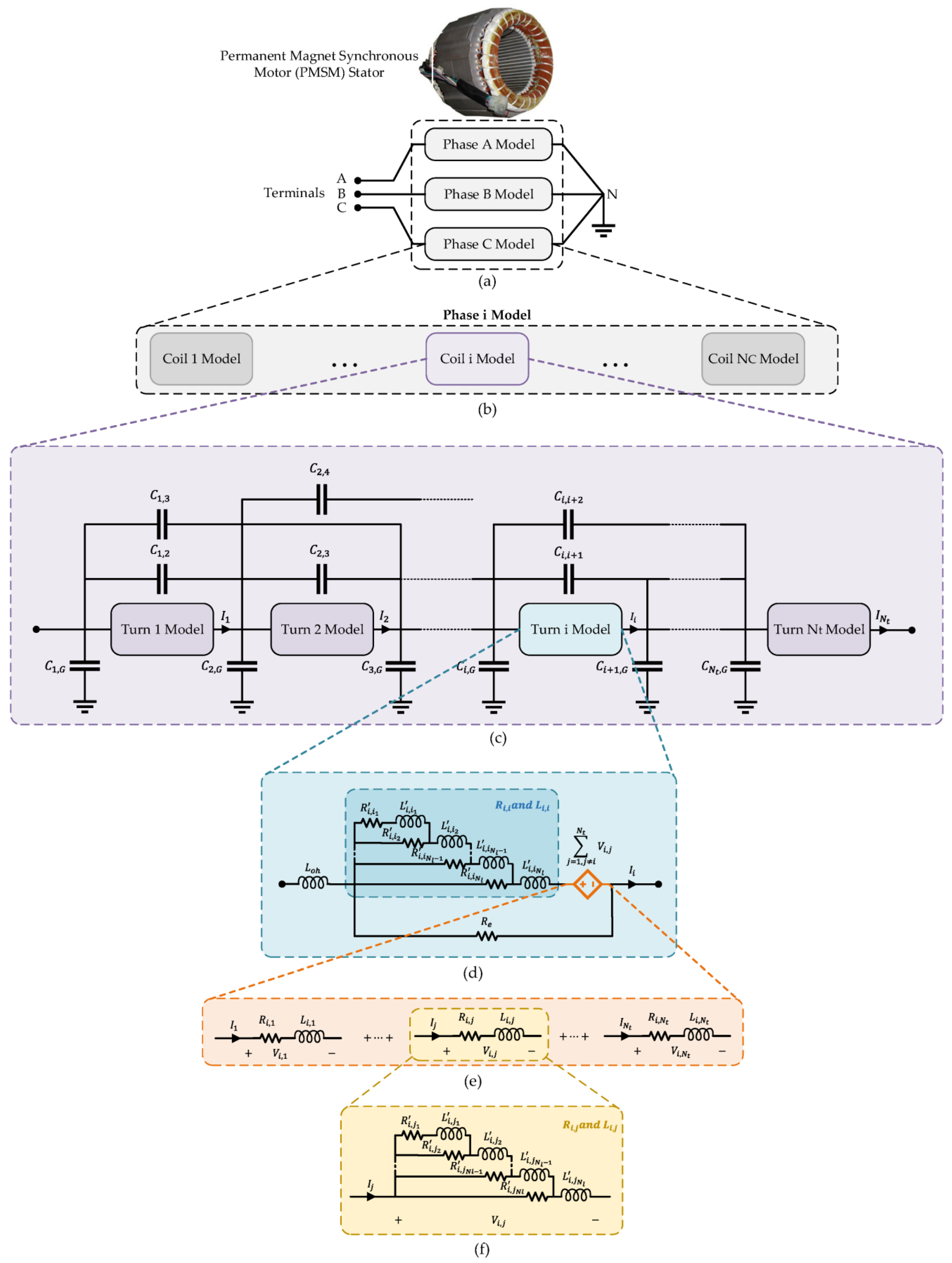
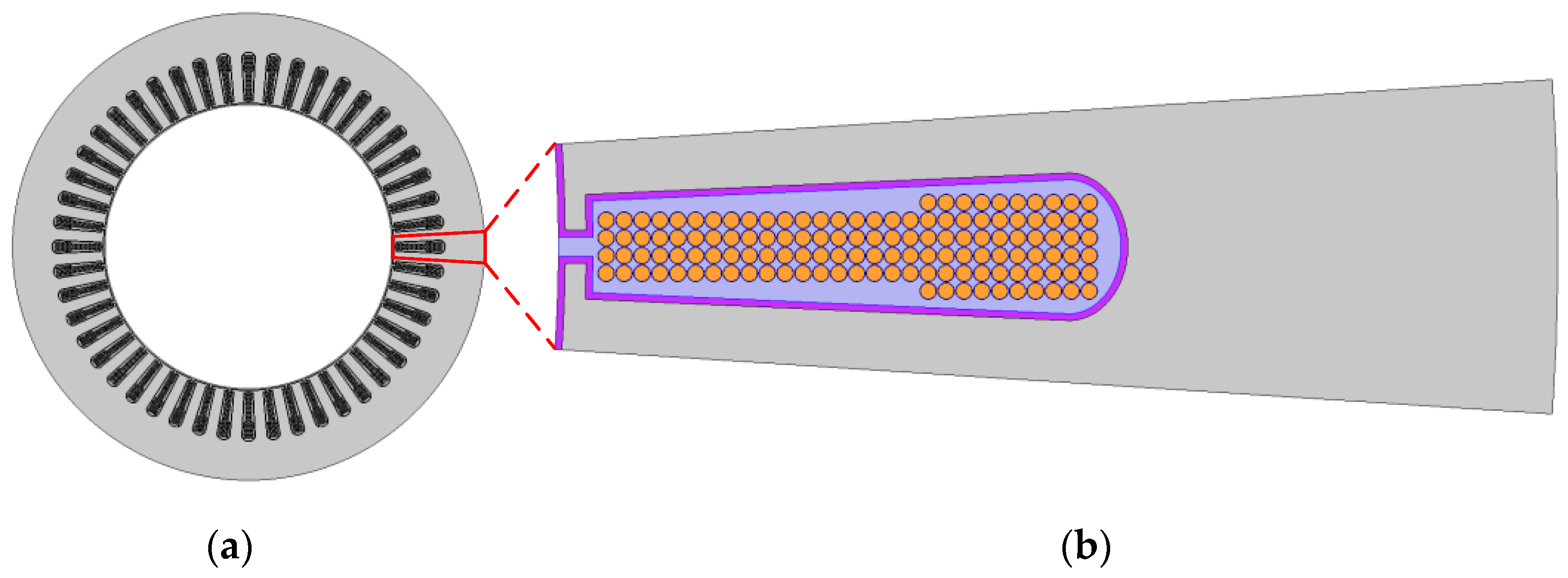
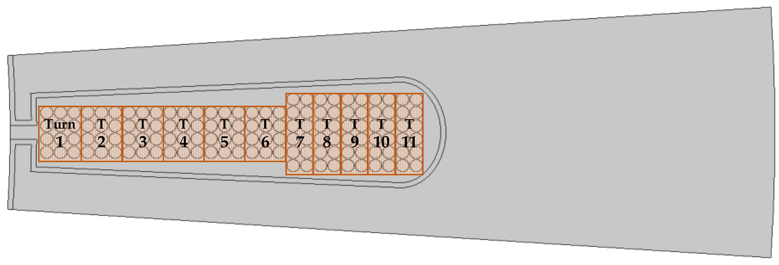
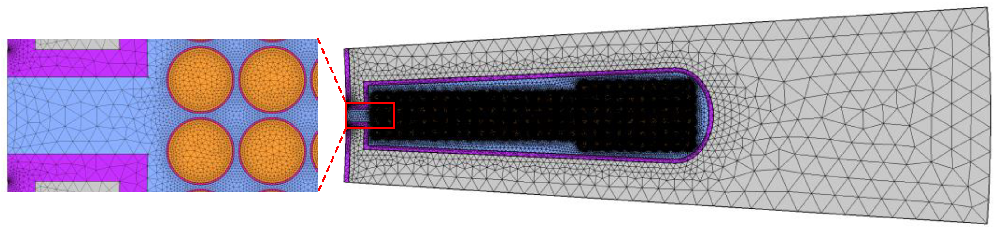
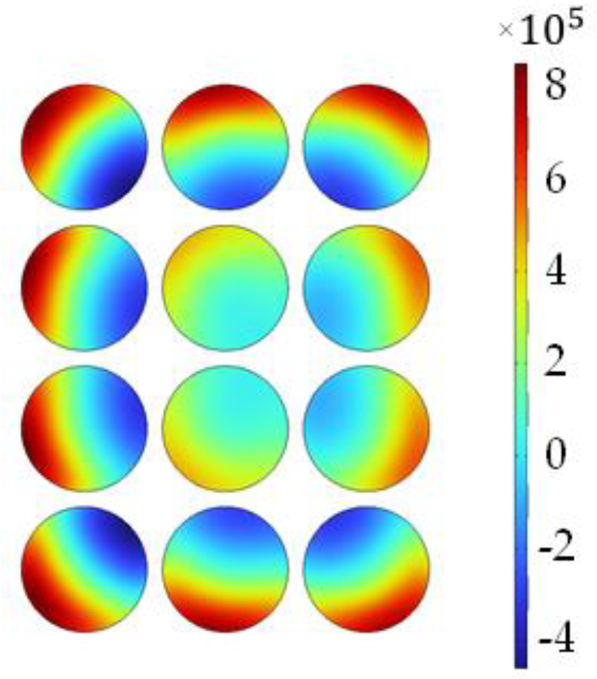

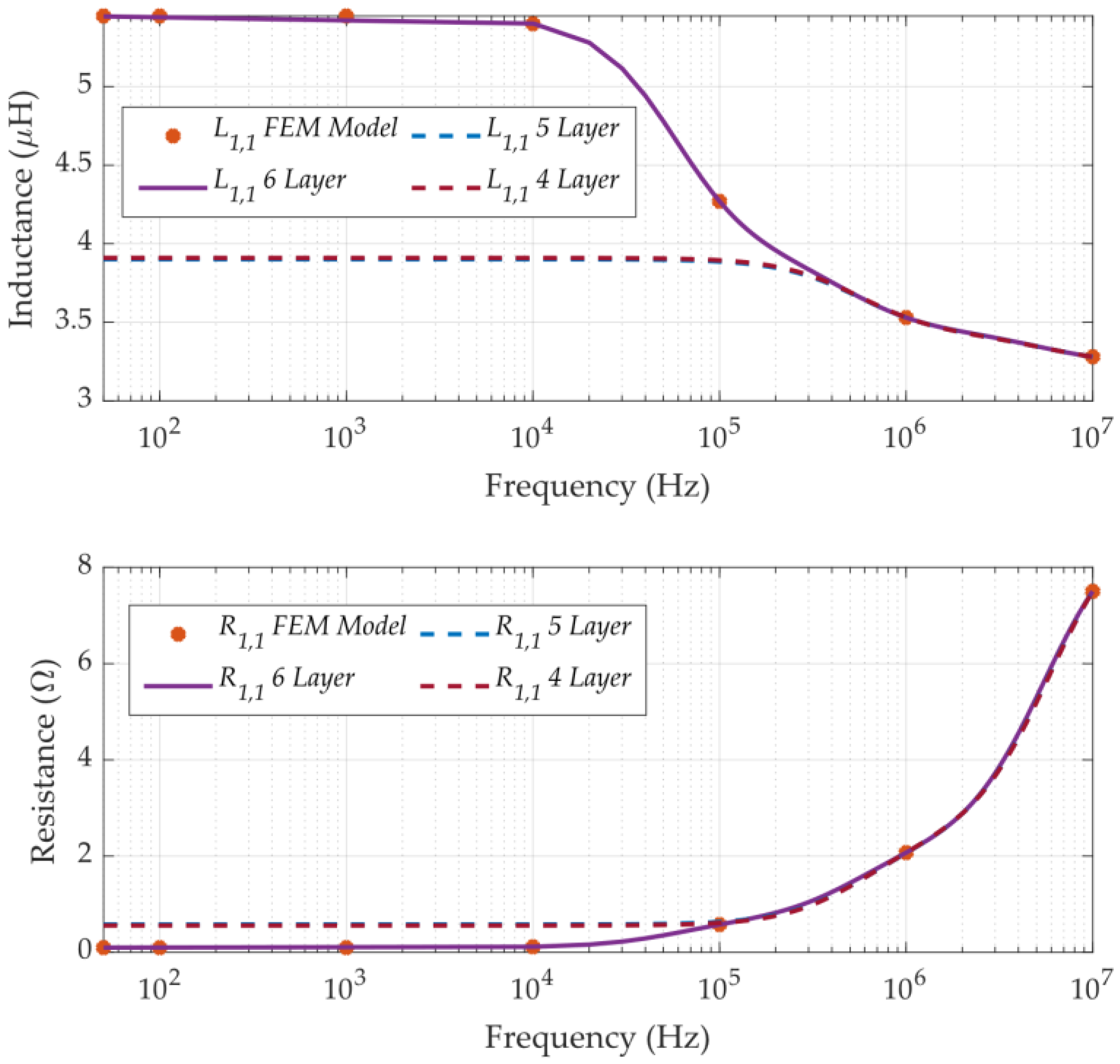


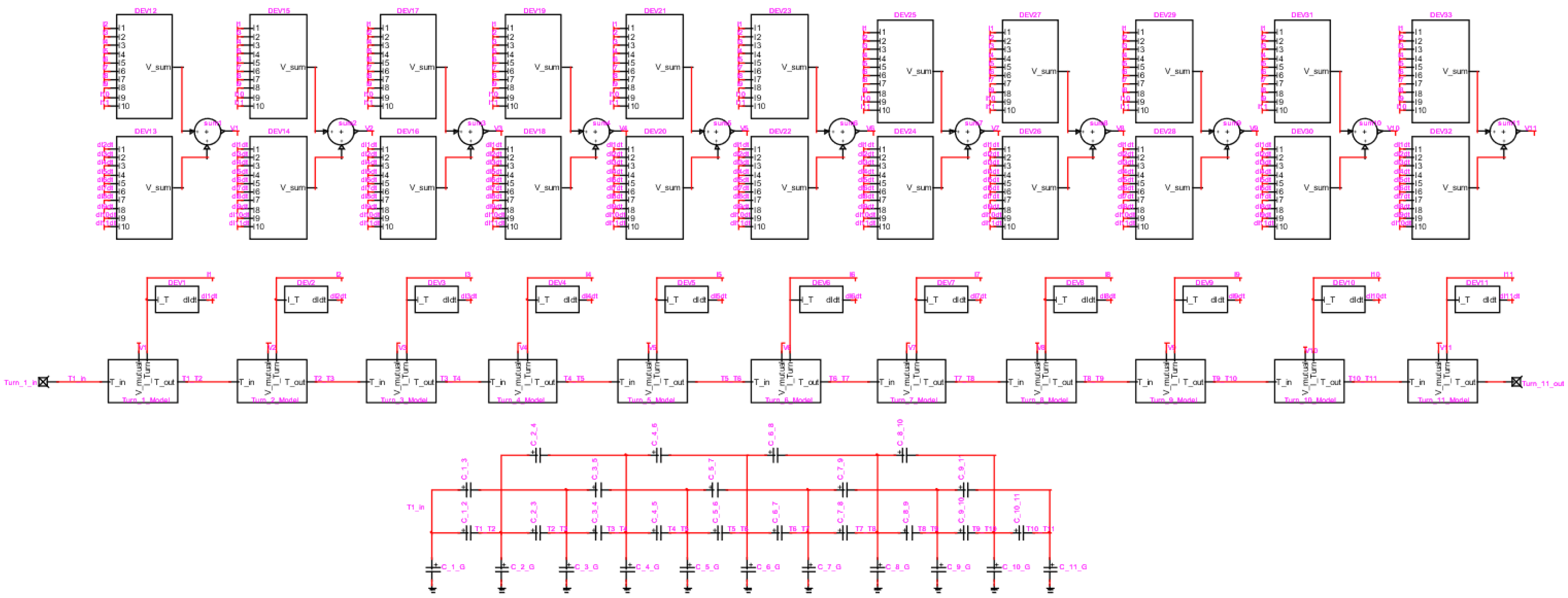
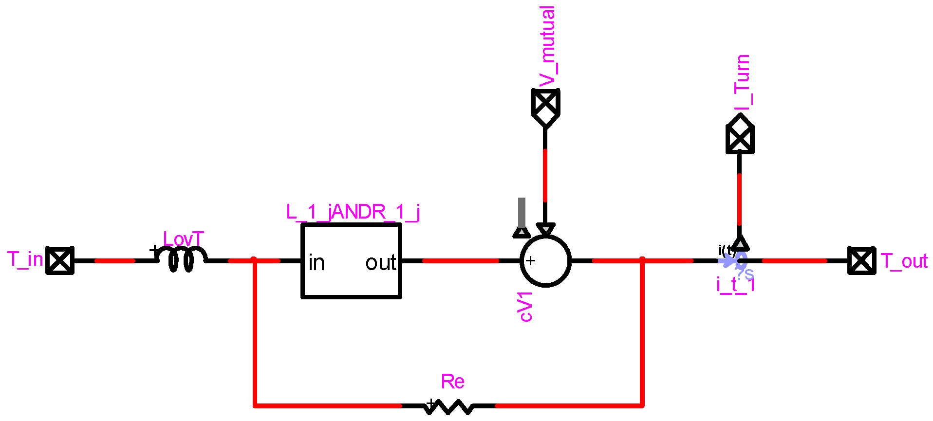
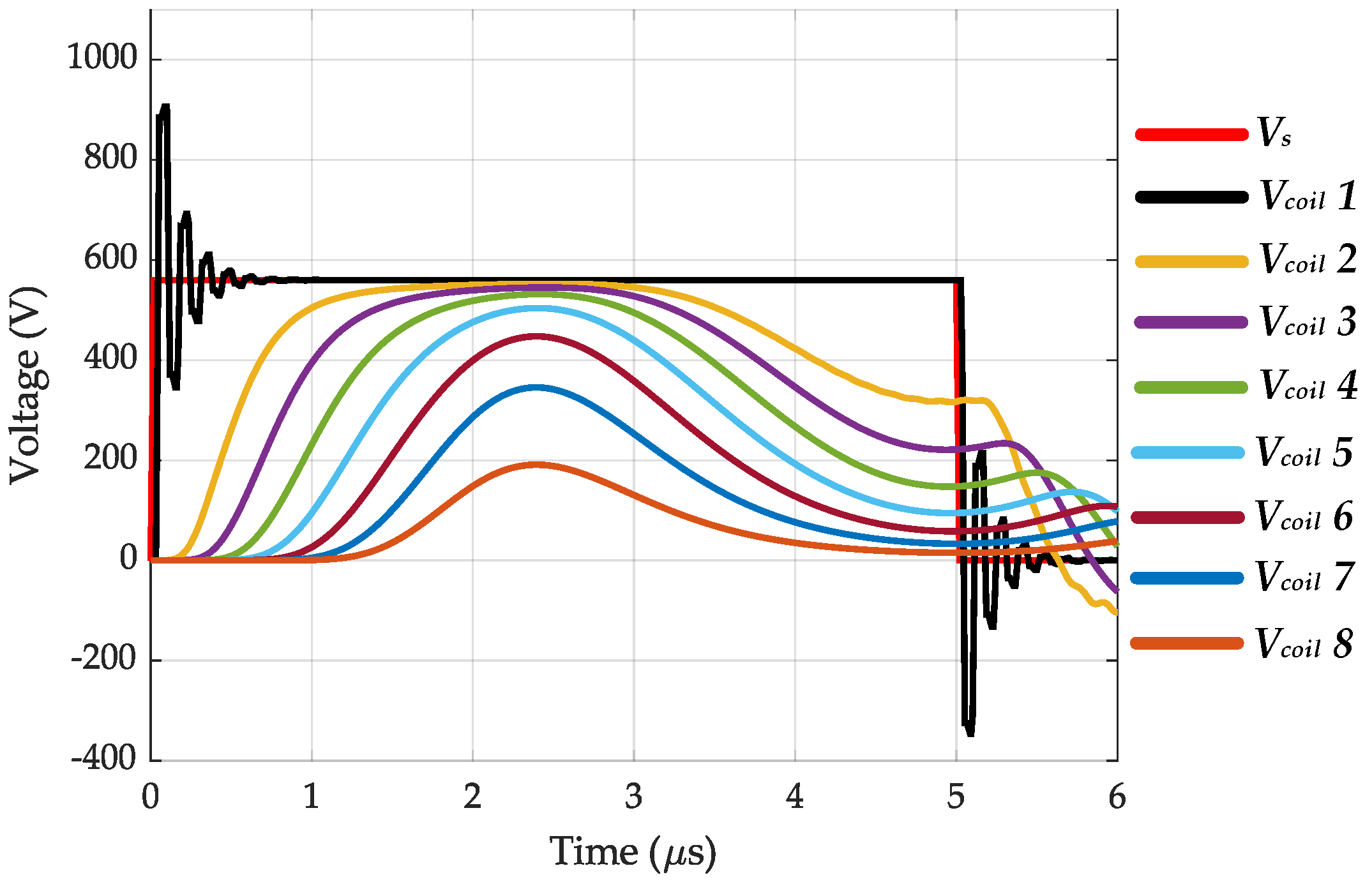
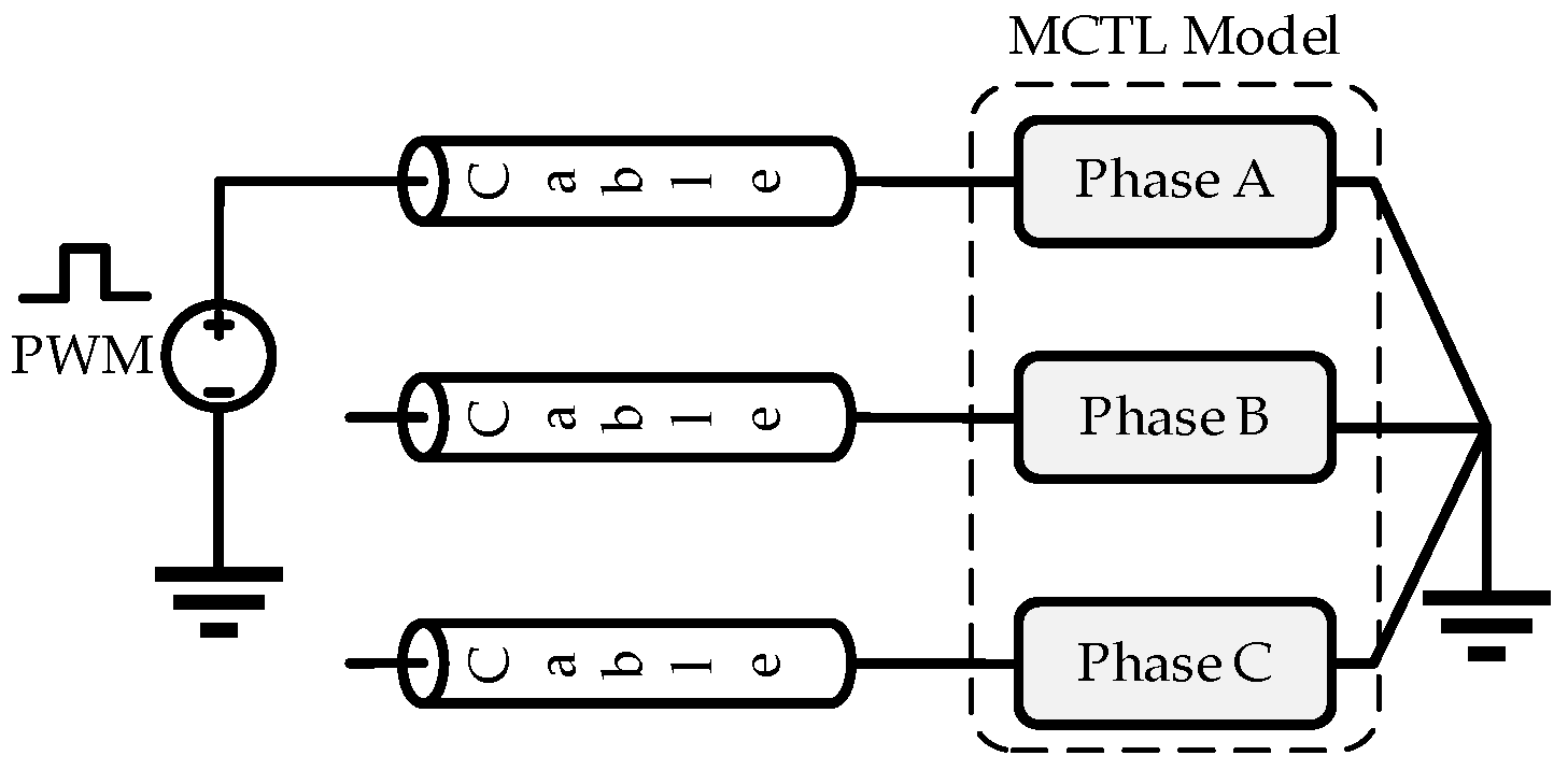
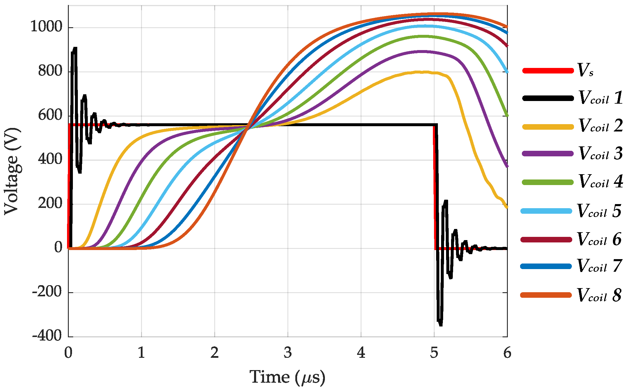
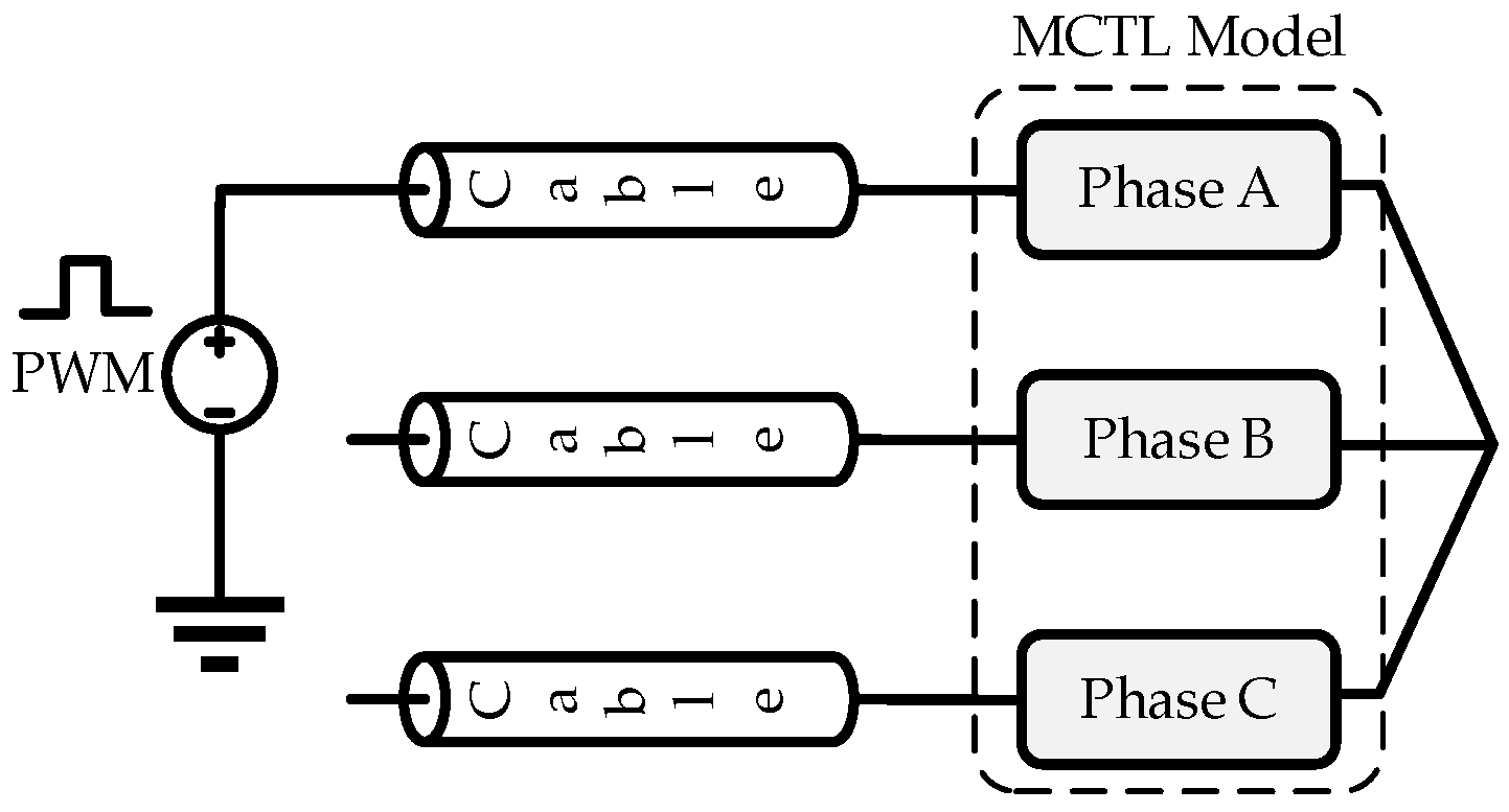
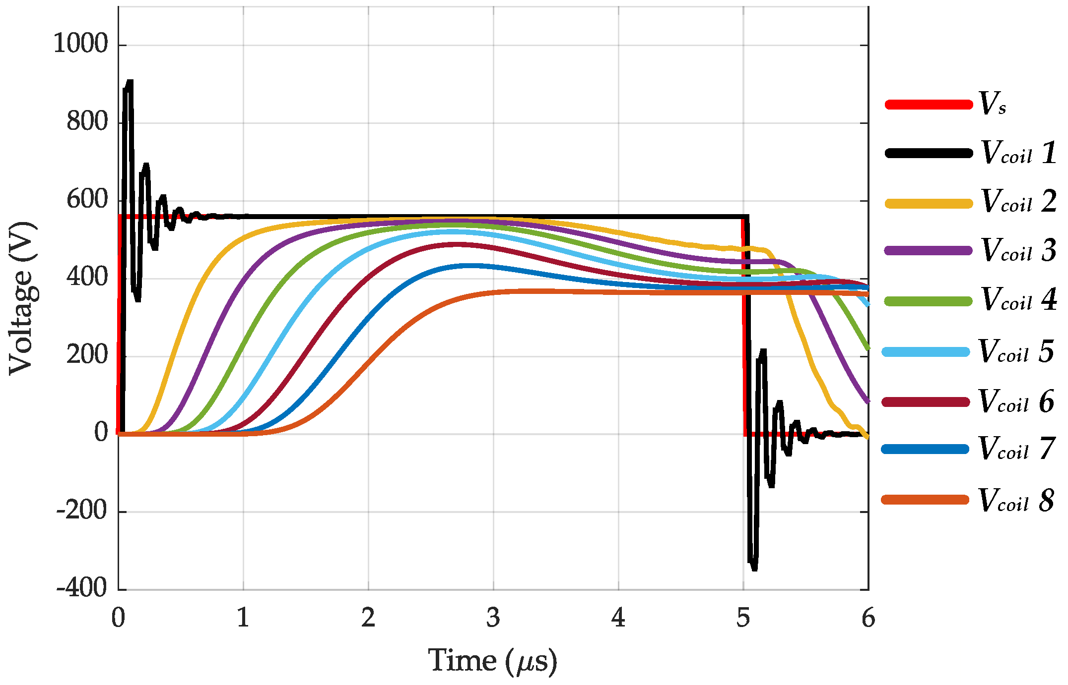
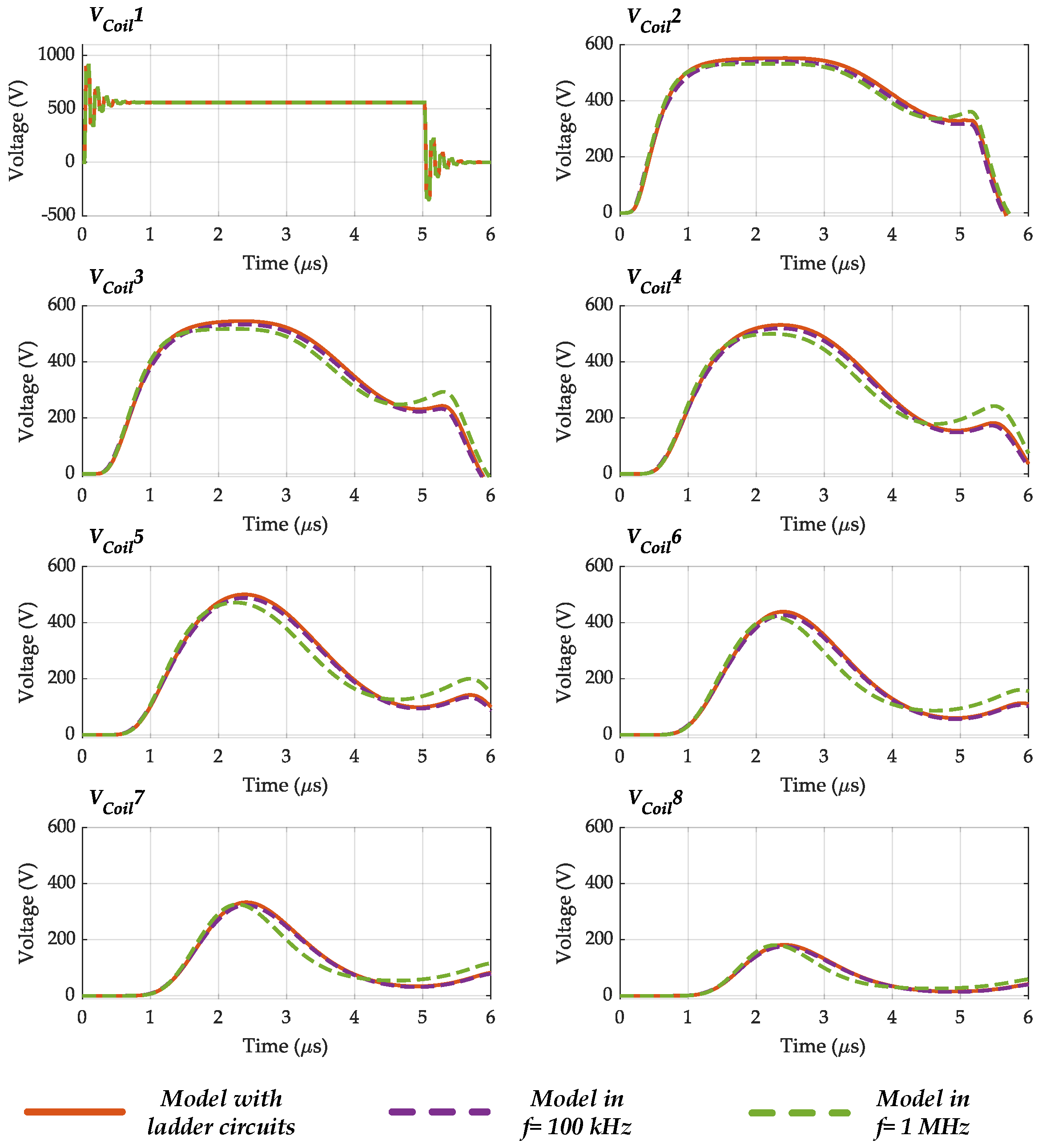
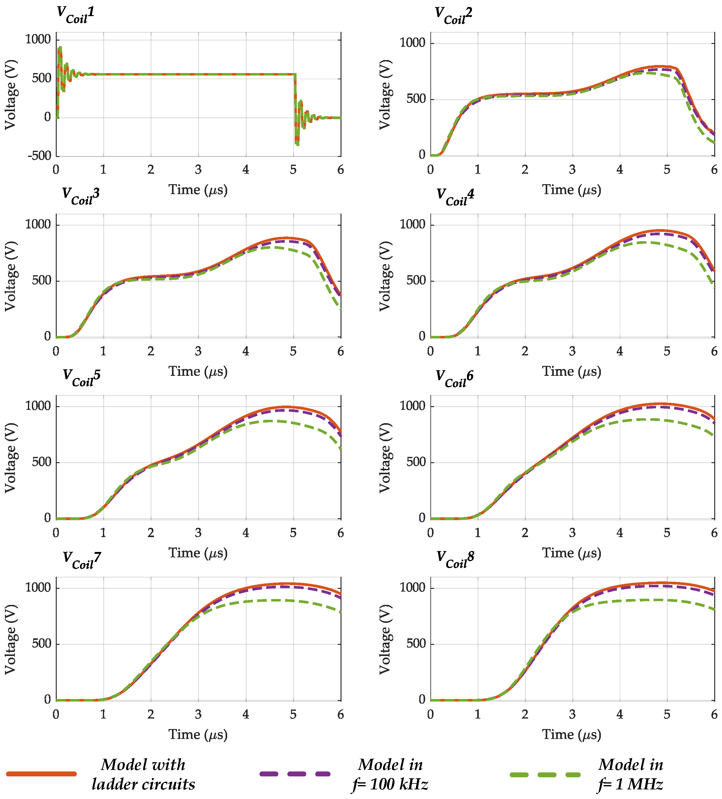
Publisher’s Note: MDPI stays neutral with regard to jurisdictional claims in published maps and institutional affiliations. |
© 2022 by the authors. Licensee MDPI, Basel, Switzerland. This article is an open access article distributed under the terms and conditions of the Creative Commons Attribution (CC BY) license (https://creativecommons.org/licenses/by/4.0/).