Smart Design: Application of an Automatic New Methodology for the Energy Assessment and Redesign of Hybrid Electric Vehicle Mechanical Components

Abstract

This work aimed to develop an automatic new methodology based on establishing if a mechanical component, designed for a conventional propulsion system, is also suitable for hybrid electric propulsion. Change in propulsion system leads to different power delivery and vehicle dynamics, which will be reflected in different load conditions acting on the mechanical components. It has been shown that a workflow based on numerical simulations and experimental tests represents a valid approach for the evaluation of the cumulative fatigue damage of a mechanical component. In this work, the front half-shaft of a road car was analyzed. Starting from the acquisition of a speed profile and the definition of a reference vehicle, in terms of geometry and transmission, a numerical model, based on longitudinal vehicle dynamics, was developed for both conventional and hybrid electric transmission. After the validation of the model, the cumulative fatigue damage of the front half-shaft was evaluated. The new design methodology is agile and light; it has been dubbed “Smart Design”. The results show that changing propulsion led to greater fatigue damage, reducing the fatigue life component by 90%. Hence, it is necessary to redesign the mechanical component to make it also suitable for hybrid electric propulsion.

1. Introduction

Nowadays, purely electric transmission is becoming increasingly popular in the automotive field [1,2]. The main advantage of this type of transmission is to cut down local pollutant emission [3,4,5,6], so as to improve air quality of urban centres and, hence, help in the reduction of global pollution. Despite the obvious advantages, many problems mean this type of architecture is still not strongly present on a global level: high vehicle costs related to a more complex architecture and control systems [7], battery autonomy [8,9,10,11] and the lack of infrastructure (charging stations) in urban centers [12,13,14]. For this reason, hybrid-electric transmission represents the main alternative awaiting more reliable and less expensive solutions. It is possible to divide hybrid electric transmissions into three main architectures: series, parallel and combined hybrid [15,16,17,18]. Typically, the architectures have an Internal Combustion Engine (ICE), an electric motor/generator, a power converter, a batteries pack, a mechanical transmission and a controller for power management. In the series configuration, the ICE is connected to the electric generator unit, which converts mechanical power into electric power used to recharge the battery pack. The possibility of decoupling the ICE from the electric motor would allow the ICE to only be used for recharging batteries, thereby running the ICE at maximum efficiency points and downsizing the engine i.e., reducing the number of cylinders with respect to a conventional configuration. In the parallel configuration, the ICE is directly connected with the transmission and a part of the mechanical power is used for generating the traction force, together with the electric power generated by the electric motor/generator. In the combined hybrid configuration, one or more electric machines work in concert with the ICE to achieve the advantages of series architecture and those of parallel configuration. The mathematical modelling of the transmission, and, in particular, the longitudinal vehicle dynamics, represents a powerful tool for the evaluation of propulsion system performance. According to the literature review [19,20,21,22,23,24], two main approaches are employed: the backward and feed-forward approaches. The backward approach consists in imposing a driving cycle on the system and, through the mathematical modelling of the transmissions, evaluating the power required from the engine. No driver is considered within the system. On the other hand, the feed-forward approach consists of inserting a driver within the system. In this case, the information’s flow is the opposite of the backward approach and inherent with reality: from the engine to the vehicle speed. Finally, the vehicle speed is matched with a reference speed (drive cycle) through a control system acting on the throttle/brake pedal position. In addition to the mathematical modelling, the increasing usage of machine learning and neural network algorithms [25,26,27,28,29] has led to new vehicle control and design strategies [30]. An important aspect to investigate is the stress state acting on the mechanical components when the vehicle is hybridized, starting from a conventional configuration i.e., only with the ICE engine propulsion. The different propulsion, transmission and weight distribution inevitably leads to different vehicle dynamics and, as a consequence, different stresses on mechanical components [31]. Hence, the initial component design, compatible with the conventional configuration, may not be suitable for the hybrid electric vehicle. To investigate the effect of different propulsion on the stresses acting on mechanical components, the authors propose a new agile and light methodology, based on automatic evaluation of the cumulative stress through the interactions of different software (multibody, FEM, etc.) and models (consumption, vehicle dynamics, structural, etc.) in the Matlab environment. This new way of verifying and re-designing mechanical components has been called “Smart Design” by the authors. Indeed, in the modern era, it is impossible to think that structural design does not make use of virtual, digital, rapid and secure prototyping methods. So, the aim is for the CPU to do multifunctional simulations in order to find the optimal result. In the specific case of this work, through the “Smart Design”, an evaluation of the cumulative fatigue damage of the front half-shaft was calculated for the purpose of redesign for hybrid propulsion. The first step was to define the reference vehicle. Then, a drive cycle was acquired through a SCADAS XS COMPACT control unit provided by the SIEMENS^TM Company, together with a GPS sensor. A mathematical model of both conventional and hybrid electric transmission was created in AVL CruiseM^TM, according to a feed-forward approach. Both models were calibrated, matching the vehicle speed to the reference speed through a feedback controller (PI type) acting on throttle/brake pedal position. Moreover, from the simulations, it was possible to evaluate the torque at the front half-shaft that would be used for evaluation of the cumulative fatigue damage. The component object of this study was tested through fatigue tests [32] with three different load levels and oscillating amplitudes i.e., load ratio R = −1. From the experimental tests, the T_a-N torsion curve (torque amplitude-number of cycles) of the component was obtained. This curve allowed for the evaluation of the fatigue life of the component subjected to a torque history. The results showed that the cumulative damage (design at 400,000 km) was around 14% for the ICE torque history, while it was around 90% for the HEV torque history. This meant that propulsion change led to more damage reducing the fatigue life of the component. Therefore, it is necessary to redesign the component for hybrid propulsion in order to ensure a better fatigue life.

2. Materials and Methods

This work aimed to develop a methodology based on evaluation of cumulative fatigue damage in order to assess a mechanical component, realized for conventional propulsion, to determine if it was also suitable for hybrid electric propulsion. Figure 1 shows the workflow adopted.

Figure 1. Workflow adopted for the evaluation of the cumulative fatigue damage of the component. It is possible to choose two different workflows, depending on the availability of the experimental data of the component.

The workflow started with the definition of the vehicle parameters, in terms of transmission and geometry, and the acquisition of the driving cycle. Then, through a numerical simulation of both transmissions (ICE and HEV), it was possible to evaluate the load cycle on the component. Depending on the availability of experimental data on the component under examination, two possible approaches existed:

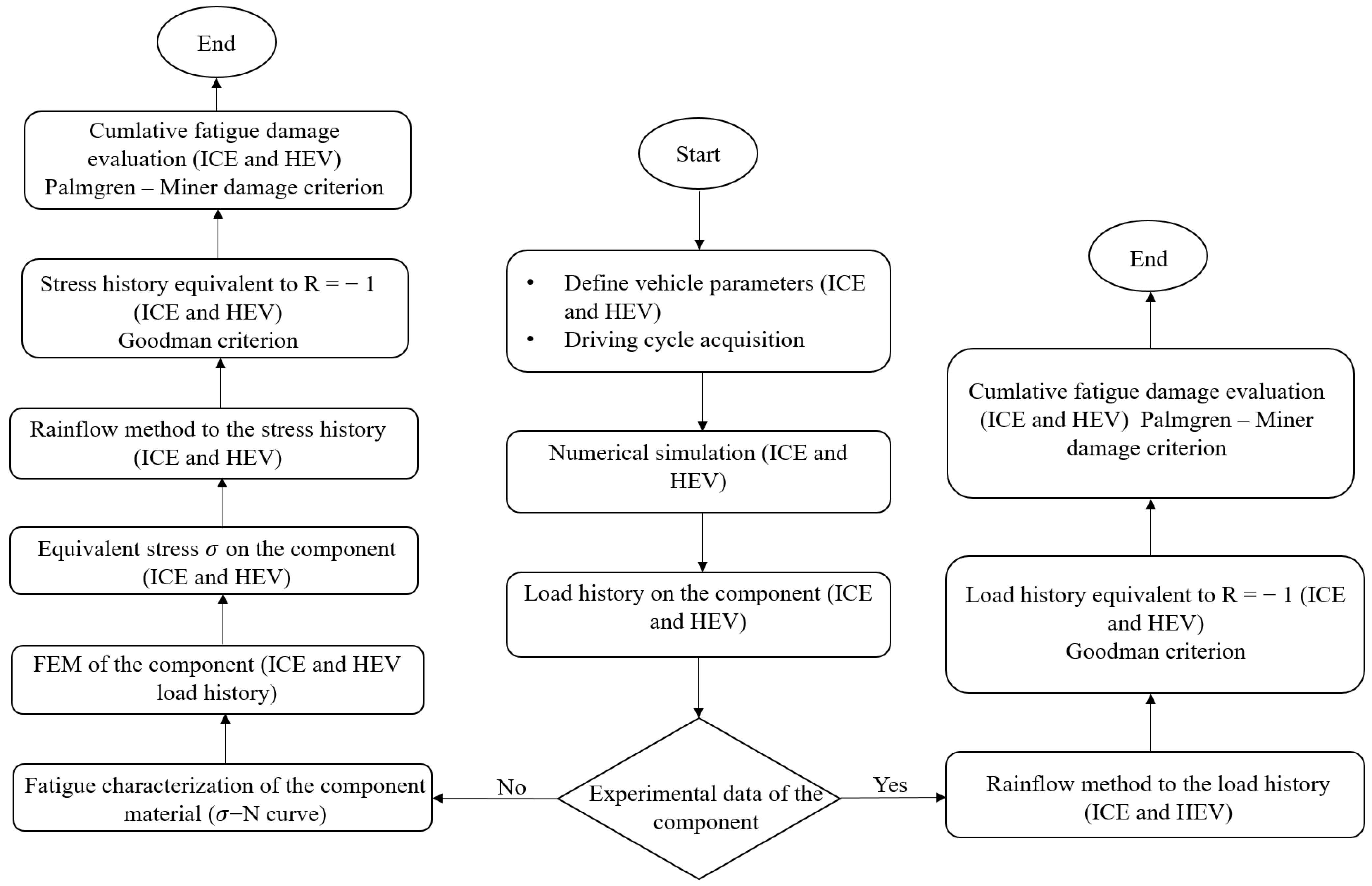
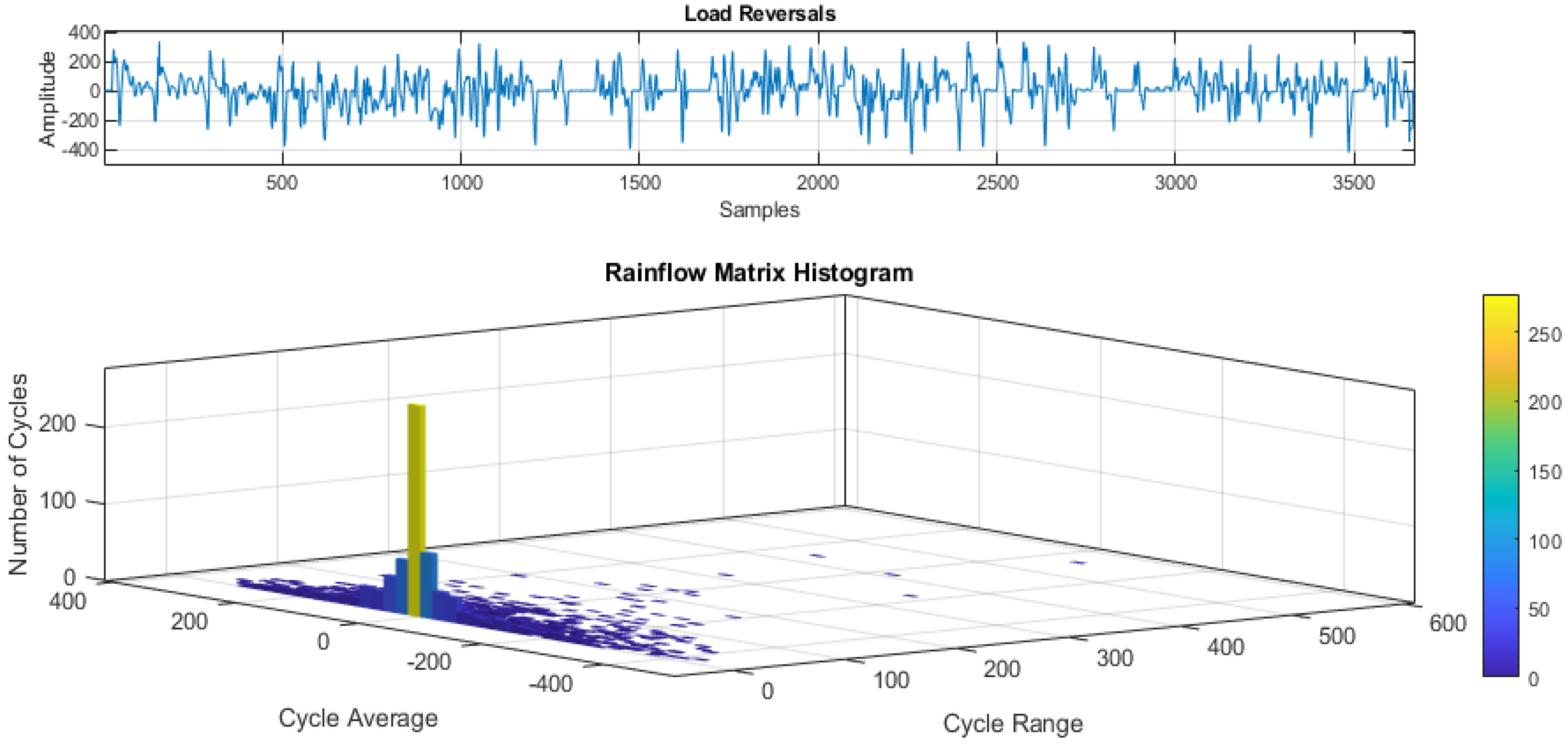
• Experimental data of the component. In this case, it was necessary, through the Rainflow method [33], to extract an equivalent load cycle in terms of stress amplitude (or, in this case, torque amplitude) and the number of cycles. Then, it was necessary to obtain an equivalent load history at load ratio R = −1, using the Goodman criterion [34]. This was done because it is common practice to test the component [32] or the material component [35] at constant amplitude. Finally, the cumulative fatigue damage was evaluated using the Palmgren-Miner criterion [36].
• No experimental data on the component. In this case, it was necessary to characterize the component material through fatigue tests, firstly. This allowed obtaining the $\sigma -N$ curve (stress amplitude-number of the cycle) of the material, which would be used for the cumulative fatigue damage calculation. Then, through a Finite Element Model (FEM) of the component, it was possible to pass from load to equivalent stress $\sigma$ on the component. Usually, for steels, the most common criterion to evaluate the equivalent stress is the Von Mises criterion [37]. At this point, the procedure followed the same steps as the previous case.

2.1. Reference Vehicle

The conventional vehicle adopted in this work was a mid-size sedan, the parameters of which are shown in Table 1.

Table 1. Reference vehicle geometry and transmission main parameters.

Parameter	Value
$m_v$, vehicle mass	1505 kg
$S_a$, frontal area	$1.77{\mathrm{m}}^2$
$C_x$, drag coefficient	0.445
$l$, wheelbase	2.817 m
$r_w$, wheel rolling radius	0.305 m
${\tau }_1$, gear ratio-1st	3.54
${\tau }_2$, gear ratio-2nd	1.92
${\tau }_3$, gear ratio-3rd	1.28
${\tau }_4$, gear ratio-4th	0.91
${\tau }_5$, gear ratio-5th	0.67
${\tau }_6$, gear ratio-6th	0.53
${\tau }_{FD}$, final drive ratio-front	4.35

Figure 2 shows the maximum torque map and the consumption map of the ICE engine adopted for the simulation.

Figure 2. Maximum torque map and consumption map of the ICE adopted in the simulation.

Hybrid Electric Vehicle

The architecture chosen for vehicle hybridization was a parallel hybrid drivetrain in P2 configuration i.e., the electric motor was placed on the driving axis (front axis). Table 2 shows the main parameters of the HEV.

Table 2. HEV geometry and transmission main parameters.

Parameter	Value
$m_v$, vehicle mass	1770 kg
$S_a$, frontal area	$1.77{\mathrm{m}}^2$
$C_x$, drag coefficient	0.445
$l$, wheelbase	2.817 m
$r_w$, wheel rolling radius	0.305 m
${\tau }_1$, gear ratio-1st	3.54
${\tau }_2$, gear ratio-2nd	1.92
${\tau }_3$, gear ratio-3rd	1.28
${\tau }_4$, gear ratio-4th	0.91
${\tau }_5$, gear ratio-5th	0.67
${\tau }_6$, gear ratio-6th	0.53
${\tau }_{FD}$, final drive ratio-front	4.35
$E_b$, battery energy	1299.5 Wh
$V_0$, battery nominal voltage	230 V
$C_b$, battery capacity	5.65 Ah

Figure 3 shows the maximum torque map of the electric motor/generator adopted for the simulation.

Figure 3. Electric machine maximum torque map.

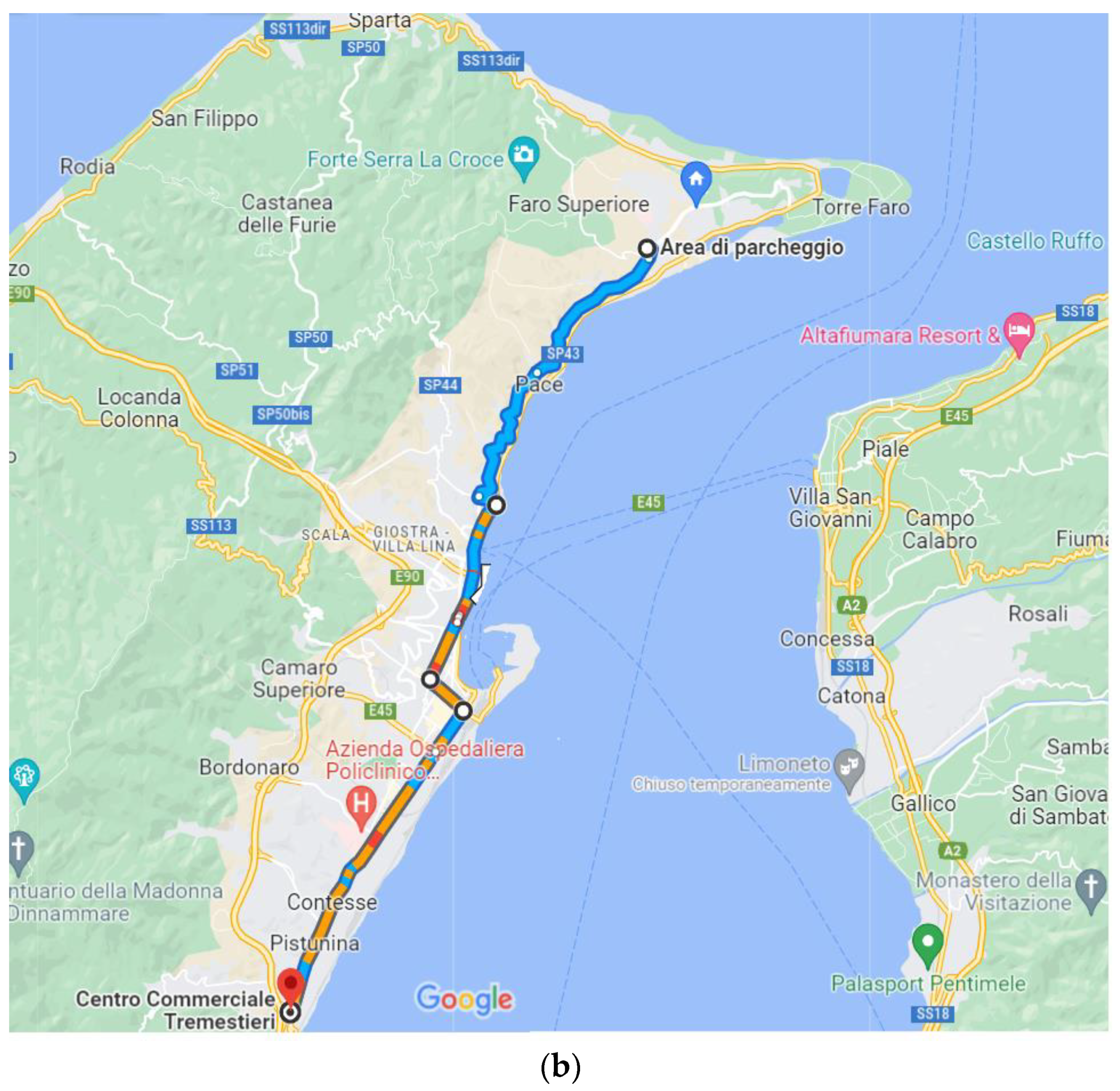
2.2. Data Acquisition

The speed profile, road inclination and vehicle position were acquired through a SCADAS XS compact control unit provided by the SIEMENS^TM Company, together with a GPS sensor. Figure 4 shows the instrumentation used for data acquisition.

Figure 4. Instrumentation used for data acquisition. It consisted of a control unit provided by the Siemens company (model SCADAS XS Compact), a GPS sensor and a tablet for the monitoring.

Figure 5a shows the speed profile and altitude, while Figure 5b shows the vehicle position.

Figure 5. Data acquisition from GPS sensor. (a) Speed profile and altitude (0 value is the sea level); (b) Vehicle position.

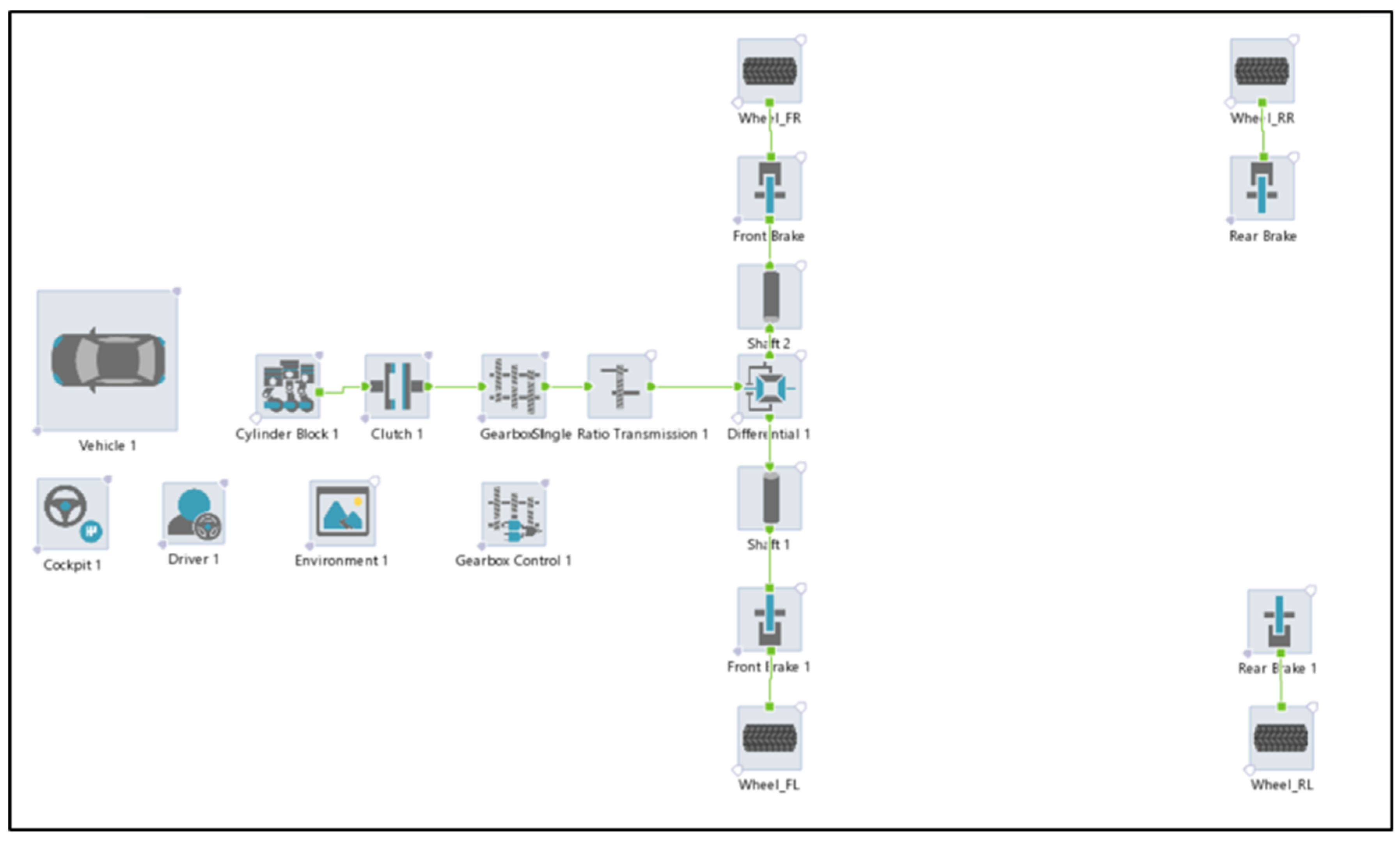
2.3. Conventional Vehicle Feed-Forward Model

The mathematical model of the conventional vehicle was based on longitudinal vehicle dynamics and the model allowed a feed-forward approach, as shown in Figure 6.

Figure 6. Conventional vehicle feed-forward model scheme. ICE: Internal Combustion Engine, Clutch, GB: gearbox, FD: final drive, ${\gamma }_{GB}$: gearbox gear ratio, $v_v$: vehicle speed, $v_{ref}$: reference speed.

The main elements were:

• Driver. The task of the driver block was to match the vehicle speed $v_v$ with the reference speed $v_{ref}$ acquired during the driving cycle, through a controller (PI type) acting on the throttle/brake pedal position.
• Internal Combustion Engine (ICE). It received the information from the cockpit block (torque command) in order to develop the required torque $T_e$.
• Clutch. The clutch block had the task of coupling/decoupling the transmission from the ICE, letting the torque $T_1$ pass or not.
• Gearbox (GB). The gearbox block allowed switching the inserted gear (and hence, gear ratios). The torque level passed from $T_1$ to $T_2={\mathsf{\gamma }}_{\mathrm{GB}}{T}_1$.
• Final drive (FD). It was the final element of the transmission and consisted of a gear ratio defined according to the datasheet. Also, in this case, the torque level passed from $T_2$ to $T_3={\tau }_{FD}{T}_2$.
• Vehicle. In the vehicle block, longitudinal vehicle dynamics equations were considered. The traction force, assumed to be applied in the longitudinal direction at the tire contact patch, would be given by the sum of the aerodynamic drag force, rolling resistance force, inertial force (chassis, wheel and engine contribution) and road inclination force.

The ICE vehicle model was developed in AVL CruiseM^TM and the functional schemes are shown in Figure 7.

Figure 7. AVL CruiseM^TM ICE vehicle model.

Through the model, it was possible to evaluate the vehicle speed, thrust force, fuel consumption and torque at the front half-shaft.

2.4. HEV Feed-Forward Model

For the HEV, the modelling followed a feed-forward approach, as shown in Figure 8.

Figure 8. HEV feed-forward model scheme. B: battery, C: control unit E: engine, EM: electric motor/generator, P: power converter, U: voltage, I: current, T: torque, $\omega$: rotational speed, ${\gamma }_{GB}$: gearbox gear ratio $v_{ref}$: reference speed, $v_v$: vehicle speed.

Figure 9 shows the HEV model developed in AVL CruiseM^TM.

Figure 9. AVL CruiseM^TM HEV model with parallel architecture and P2 configuration.

The driving modes managed by the control unit were:

• Full electric mode. The vehicle ran in full electric mode and the power flow was B-P-EM-GB-FD-drive axis. This driving mode was activated when the batteries had a sufficiently high state of charge and the driving cycle was not so hard as to require the intervention of the ICE (for example, urban driving).
• Hybrid electric mode or power assist. The vehicle ran in hybrid mode and the thrust force was due to the combined action of both the electric motor and thermic motor.
• Battery recharging. The vehicle ran in hybrid mode but a part of the electric energy was used for battery recharging.
• Regenerative braking. The electric machine recovered the braking force by acting as generator and recharging the batteries.
• Full thermic mode. The vehicle ran in full thermic mode when the speed was such as to bring the electric motor into the overspeed condition.

Through the model, it was possible to evaluate the vehicle speed, thrust force, fuel consumption, state of charge of the batteries and torque at the front half-shaft.

2.5. Cumulative Fatigue Damage Evaluation

Among the available outputs of the numerical simulation for both the ICE vehicle and the HEV model, the torque at the front half-shaft was the one used to calculate the cumulative fatigue damage of the component for both cases. This was done because, considering the actual operation of the component, the twisting torque represented the heaviest stress on the component. Experimental fatigue tests were carried out on the component [32]. The component was tested with three tests at three different load levels with a constant load ratio of R = −1, defined in Equation (1):

$$R=\frac{T_i}{T_s}=-1$$

(1)

where $T_s$ is the superior limit torque while $T_i$ is the inferior limit torque. The definition of average torque and range torque were also considered, defined in Equations (2) and (3), respectively:

$$T_m=\frac{T_s+T_i}{2}$$

(2)

$$T_a=\frac{T_s-T_i}{2}$$

(3)

Equation (1) also means that $T_m=0$. The experimental results allowed the obtaining of the T_a-N curve (torque amplitude-number of cycles) of the mechanical component. In addition, it was necessary to fit the experimental tests to have a linear trend in a bi-logarithmic diagram, also called the Wöhler diagram [35]. Linear fitting was performed using the Basquin equation [38,39], defined in Equation (4):

$$T_a=2^b{T}_f^{\prime }{N}_f^b$$

(4)

where $T_a$ are the ranges of torque, $T_f^{\prime }$ is approximately equal to the twisting torque at the break, $N_f$ are the failure cycles and $b$ is a constant. As a matter of fact, the torque history evaluated from the numerical simulation represented a random load in the time domain. As a consequence, it was necessary to extrapolate from the starting load history, an equivalent load history referred at R = −1, in order to evaluate the fatigue damage. At first, the Rainflow method [33] was applied to the load history. Through this method it was possible to obtain much load history characterized by a certain torque range $T_a$, torque mean $T_m$, number of working cycle $N$ and load ratio $R$ which, in the vast majority of cases, turned out to be different to $R=-1$. Hence, in order to convert all the load histories into an equivalent one at $R=-1$, the Goodman criterion [34] was applied. It is defined in Equation (5):

$$\frac{T_a}{T_{ar}}+\frac{T_m}{T_u}=1$$

(5)

where $T_a$ is the torque range computed from the Rainflow method, $T_{ar}$ is the equivalent torque range referred at $R=-1$, $T_m$ is the torque mean evaluated from the Rainflow method and $T_u$. is the twisting torque at the break. Finally, it was possible to evaluate the cumulative fatigue damage by applying the Palmgren-Miner criterion [36], defined in Equation (6):

$${{\displaystyle \sum }}_i\frac{N_i}{N_{fi}}=1$$

(6)

where $N_i$ are the number of working cycles and $N_{fi}$ are the corresponding failure cycles.

3. Results

In this section, the main results of the proposed methodology will be presented. In the first results part, a comparison between the ICE and the HEV model was performed from an energetic point of view. Then, starting from the torque history evaluated from the numerical simulation, the cumulative fatigue damage of the front half-shaft was evaluated for both configurations.

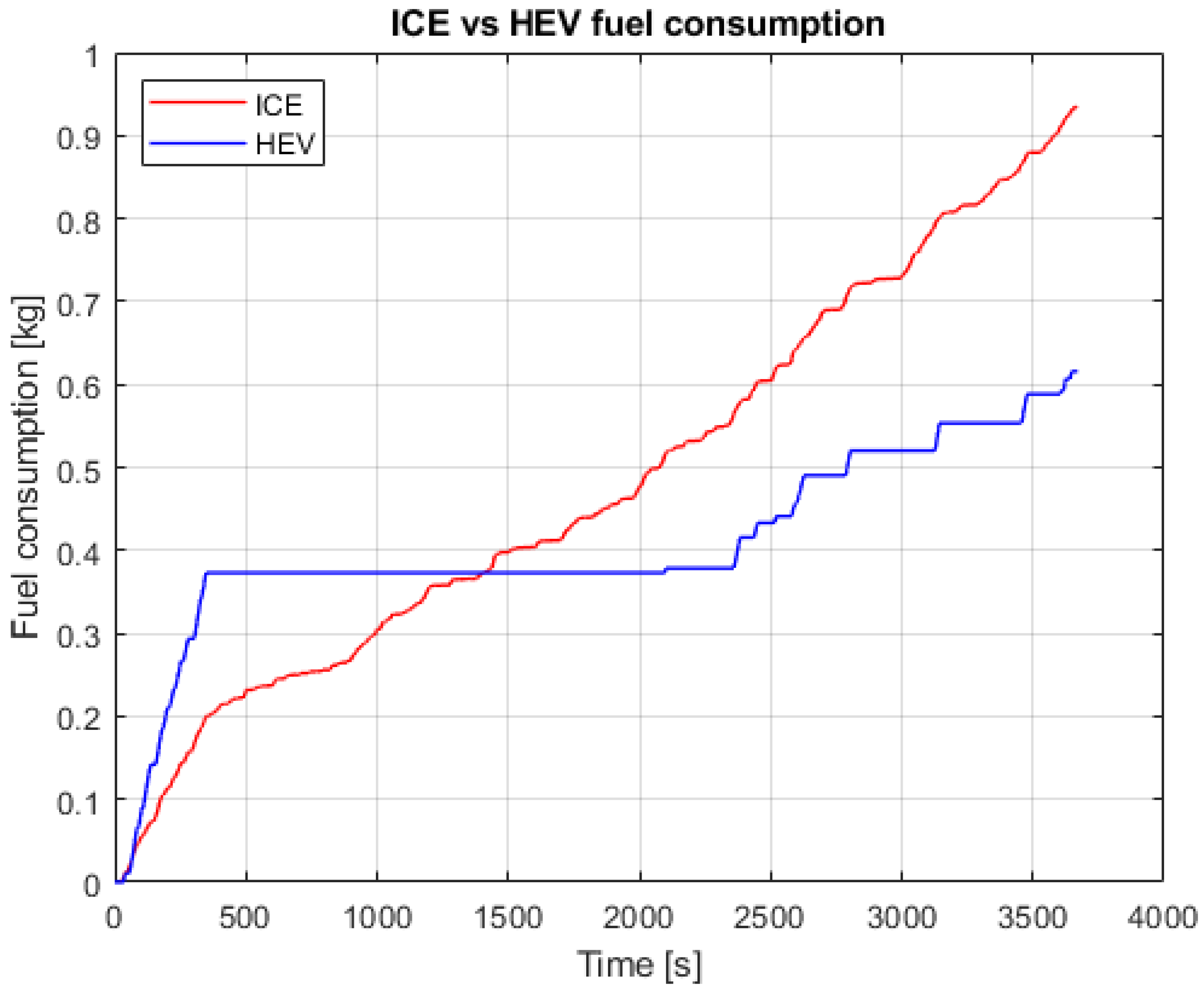
3.1. ICE Vehicle Model and HEV Model Energetic Comparison

To calibrate the model based on the acquired data, the vehicle must follow the imposed driving cycle shown in Figure 1a. To allow the vehicle to follow the speed profile, a feedback controller (PID type) was designed to act on the throttle/brake pedal position. The gains used for the controller are shown in Table 3, while in Figure 10 shows the comparison between the reference and the vehicle speed for both configurations.

Table 3. Gains used for feedback controller design.

Parameter	Value
P, proportional gain	10
I, integrative gain	0.2

Figure 10. Comparison between reference speed and vehicle speed for both configurations.

After matching the reference speed with the vehicle speed, the thrust force $F_t$ was evaluated. It took into account the following contributions:

• Aerodynamic friction losses (drag force)
• Rolling friction loss, the energy dissipated in the brakes
• Force caused by gravity when driving on non-horizontal roads
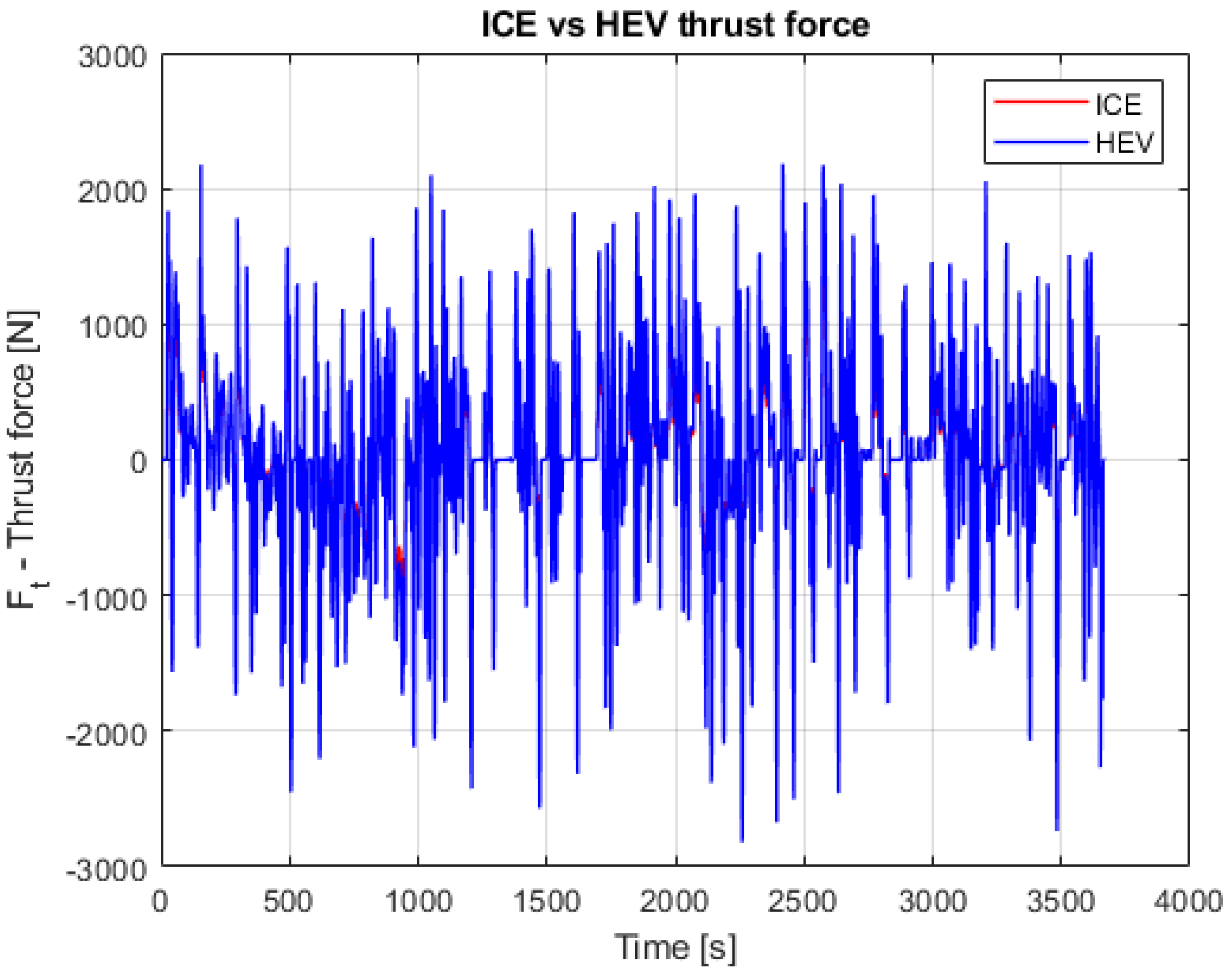
• Thrust force for both configurations, as shown in Figure 11.

Figure 11. Thrust force comparison between ICE vehicle model and HEV model.

Figure 11. Thrust force comparison between ICE vehicle model and HEV model.

The state of charge of the batteries was managed by a control system that switched the generator on or off in function of the driving cycle request. The control strategy was designed so that the vehicle had a residual state of charge of approximately 40% at the end of the driving cycle, in order not to damage the batteries. In order to consider a complete charge/discharge cycle of the batteries, until the same state of charge was achieved at the end of the driving cycle, so as to calculate fuel consumption of the HEV, the highlighted time laps in Figure 12 were considered.

Figure 12. State of charge of the batteries and generator state (1 on, 0 off). Highlighted, the time laps considered for the fuel consumption evaluation.

Figure 13 shows the comparison of fuel consumption for both configurations.

Figure 13. Fuel consumption evaluation for ICE vehicle model and HEV vehicle model.

Taking into account the consideration mentioned in Figure 12, the average fuel consumption expressed in km/L is shown in Table 4.

Table 4. Average fuel consumption comparison for both configurations.

Parameter	Value (ICE)	Value (HEV)
Considered total distance	17.28 km	16.09 km
Fuel consumption	0.9 kg	0.5 kg
Fuel density (Diesel)	0.835 kg/L	0.835 kg/L
Average fuel consumption	15.44 km/L	27.71 km/L

Finally, Figure 14 shows the torque at the front half-shaft (driving axis) that would be used for the fatigue damage calculation.

Figure 14. Torque history at the front half-shaft for both configurations.

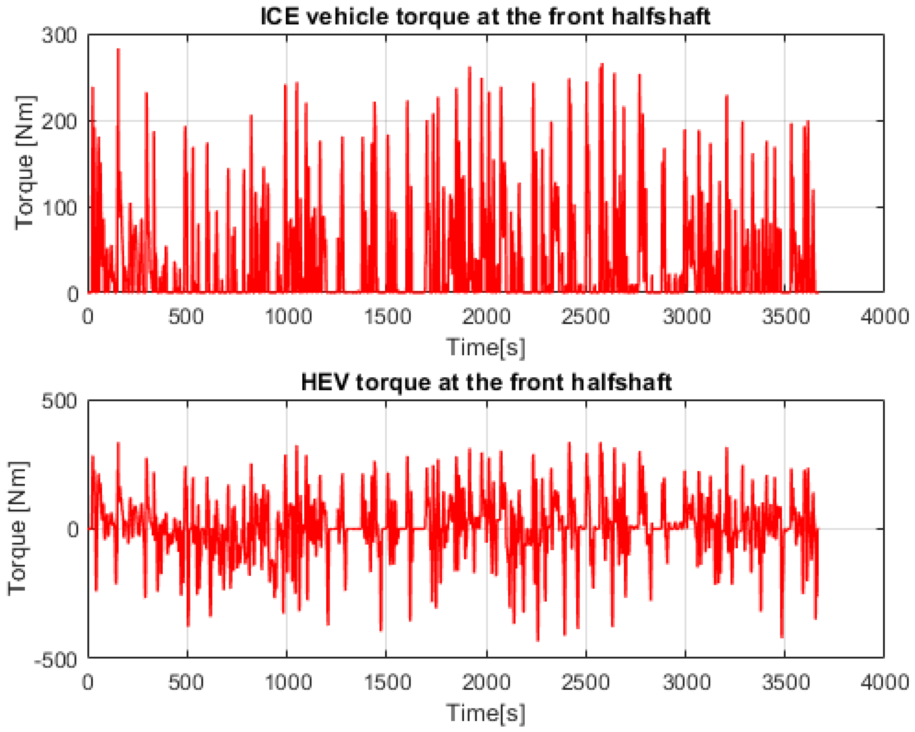
3.2. ICE Vehicle Model and HEV Model Mechanical Comparison

As described in Section 2.5, the front half-shaft was tested through fatigue tests with three tests at three different twisting torque levels and a load ratio of $R=-1$. Moreover, the experimental results were interpolated using the Basquin equation, defined in Equation (4). Figure 15 shows the experimental fatigue tests carried out on the component. The torque amplitude values were normalized concerning the maximum value for industrial reasons of secrecy.

Figure 15. Experimental fatigue test results conducted on the front half-shaft.

Then, the Rainflow method was applied to both the torque history of the ICE vehicle model and the HEV model. In addition, the mechanical design foreseen referred to the load histories to 400,000 km. Considering that the distance of the acquired driving cycle was around 17 km, the load histories must be repeated for (Equation (7)):

$$n=\frac{\mathrm{400,000}}{17}\approx \mathrm{23,000} counts$$

(7)

The application of the Rainflow method allowed the obtaining of a 3D Rainflow histogram for both configurations. It was characterized by torque range, mean torque, and number of cycles. Figure 16 shows the Rainflow histogram of the ICE vehicle model’s torque history.

Figure 16. Rainflow histogram of the ICE vehicle model torque history.

As an example, considering the high number of equivalent load histories, Table 5 shows the first ten load histories from the Rainflow method’s counting.

Table 5. First ten load histories from Rainflow method counting (ICE vehicle model).

$\mathbf{Torque}\mathbf{Range}{\mathit{T}}_{\mathit{a}}\left[\mathbf{Nm}\right]$	$\mathbf{Torque}\mathbf{Mean}{\mathit{T}}_{\mathit{m}}\left[\mathbf{Nm}\right]$	$\mathbf{Cycles}\mathit{N}$	$\mathbf{Superior}\mathbf{Torque}{\mathit{T}}_{\mathit{s}}\left[\mathbf{Nm}\right]$	$\mathbf{Inferior}\mathbf{Torque}{\mathit{T}}_{\mathit{i}}\left[\mathbf{Nm}\right]$	$\mathbf{Load}\mathbf{Ratio}\mathit{R}$
22.5	20	34,500	42.5	−2.5	−0.05
25	20	57,500	45	−5	−0.1
27.5	20	69,000	47.5	−7.5	−0.15
32.5	20	11,500	52.5	−12.5	−0.23
35	20	11,500	55	−15	−0.27
0	40	1,000,500	40	40	1
2.5	40	529,000	42.5	37.5	0.88
5	40	506,000	45	35	0.77
7.5	40	218,500	47.50	32.5	0.68
10	40	149,500	50	30	0.60

Figure 17 shows the Rainflow histogram of the HEV model torque history.

Figure 17. Rainflow histogram of the HEV model torque history.

Table 6 shows the first ten load histories from the Rainflow method’s counting.

Table 6. First ten load histories from Rainflow method counting (HEV model).

$\mathbf{Torque}\mathbf{Range}{\mathit{T}}_{\mathit{a}}\left[\mathbf{Nm}\right]$	$\mathbf{Torque}\mathbf{Mean}{\mathit{T}}_{\mathit{m}}\left[\mathbf{Nm}\right]$	$\mathbf{Cycles}\mathit{N}$	$\mathbf{Superior}\mathbf{Torque}{\mathit{T}}_{\mathit{s}}\left[\mathbf{Nm}\right]$	$\mathbf{Inferior}\mathbf{Torque}{\mathit{T}}_{\mathit{i}}\left[\mathbf{Nm}\right]$	$\mathbf{Load}\mathbf{Ratio}\mathit{R}$
45	−40	46,000	5	−85	−17
87.5	−40	11,500	47.5	−127.5	−2.68
112.5	−40	11,500	72.5	−152.5	−2.10
202.5	−40	11,500	162.5	−242.5	−1.49
0	−20	1,978,000	−20	−20	1
2.5	−20	552,000	−17.5	−22.5	1.28
5	−20	345,000	−15	−25	1.6
7.5	−20	253,000	−12.5	−27.5	2.2
10	−20	230,000	−10	−30	3
12.5	−20	69,000	−7.5	−32.50	4.3

In order to evaluate the fatigue damage, it was necessary to obtain an equivalent load history referred to $R=-1$ for both configurations, using the Goodman criterion, defined in Equation (5). Figure 18 shows the equivalent load history in the $T_a-N$ curve for the ICE vehicle model. Only the torque level above the fatigue limit, settled to $5\times {10}^6$ cycles according to literature review [35], were considered. This was decided because below the fatigue limit the mechanical component could be considered, from a theoretical point of view, to have an infinite life and, hence, these torque values did not influence the fatigue life of the component.

Figure 18. ICE vehicle model torque history referred to $R=-1$ through the Goodman criterion.

Table 7 shows the values of $\frac{T_a}{T_{a max}}$, working cycles $N$ and the corresponding failure cycles $N_f$.

Table 7. Torque amplitude, working cycles and failure cycles for the ICE vehicle model.

$\frac{{\mathit{T}}_{\mathit{a}}}{{\mathit{T}}_{\mathit{a} \mathit{m}\mathit{a}\mathit{x}}} \left[\mathit{\%}\right]$	$\mathbf{Working}\mathbf{Cycles}\mathit{N}$	$\mathbf{Failure}\mathbf{Cycles}{\mathit{N}}_{\mathit{f}}$
45.4	11,500	3951282.5
48	11,500	2889408.1
49.4	23,000	2516954.1
60.6	11,500	919579.2
63.4	34,500	833674.3
66.3	46,000	747769.4
45.8	11,500	3752326.1
49.2	11,500	2553792.5

By applying the Palmgren-Miner criterion it was possible to calculate the fatigue damage (Equation (8)):

$${\displaystyle \sum }_{i=1}^8\frac{N_i}{N_{fi}}=0.1390\cong 14\%$$

(8)

Figure 19 shows the equivalent load history in the $T_a-N$ for the HEV model through the application of the Goodman criterion:

Figure 19. HEV model torque history referred to $R=-1$ through the Goodman criterion.

Table 8 shows the values of $\frac{T_a}{T_{a max}}$, working cycles $N$ and the corresponding failure cycles $N_f$.

Table 8. Torque amplitude, working cycles and failure cycles for the HEV mode.

$\frac{{\mathit{T}}_{\mathit{a}}}{{\mathit{T}}_{\mathit{a} \mathit{m}\mathit{a}\mathit{x}}} \left[\mathit{\%}\right]$	$\mathbf{Working}\mathbf{Cycles}\mathit{N}$	$\mathbf{Failure}\mathbf{Cycles}{\mathit{N}}_{\mathit{f}}$
54.3	11,500	1,546,168.7
102.8	11,500	69,226.8
45.48	11,500	3,917,411.8
81.8	11,500	274,118.1
49.5	11,500	2,488,406.4
50.6	11,500	2,186,339.2
49.4	11,500	2,498,245.4
55.4	11,500	1,375,488.1
78.5	11,500	374,097.2
56.1	11,500	1,286,968.4
127.1	11,500	20,284.3
49.2	23,000	2,566,367.9
69.2	23,000	657,144.8
59.2	11,500	962,304.3

By applying the Palmgren-Miner criterion it was possible to calculate the fatigue damage (Equation (9)):

$${\displaystyle \sum }_{i=1}^{14}\frac{N_i}{N_{fi}}=0.9038\cong 90\%$$

(9)

4. Discussion

The comparison of both vehicle configurations from the energetic point of view showed that both models were calibrated on the basis of the speed profile acquired experimentally. Figure 10, in fact, shows a near perfect adhesion between the vehicle speed computed from the numerical simulation and the acquired speed profile. Figure 13 shows the fuel consumption comparison for both configurations. As expected, the HEV exhibited a lower average fuel consumption, which was around 27.71 km/L at the end of the driving cycle. The ICE vehicle exhibited a greater average fuel consumption, which was around 15.44 km/L at the end of the driving cycle. Hence, despite the more complex transmission architecture of the HEV, it saved more fuel, also, thereby, reducing emission of pollutants. This was also possible due to the control strategy that managed the State of Charge of the batteries. As shown in Figure 12, the control strategy managed the State of Charge through switching the generator on or off in function of the driving cycle request and according to the driving mode exposed in Section 2.4, with a residual State of Charge of around 40% at the end of the driving cycle. The torque at the front half-shaft, shown in Figure 14, represents the connection with the mechanical point of view. As expected, the torque evaluated for the ICE vehicle was always positive. This was due to the fact that the braking force was due to the brake callipers only. Possibly, there was some resistant mechanical torque of minor entity that was neglected in this study. On the other hand, the torque evaluated for the HEV also exhibited the negative part. This was due to the regenerative braking in which the electric machine acted as a generator (Figure 3). The experimental fatigue tests, shown in Figure 15, exhibited a low data dispersion for higher torque amplitude ratio, while it increased for lower values close to the fatigue limit of the mechanical component. The application of the Palmgren-Miner criterion to both load histories showed that the changing propulsion led to greater fatigue damage on the mechanical component. As shown in Equation (7) and Equation (8), respectively, the ICE vehicle load history led to 14% fatigue damage on the component, while the HEV load history led to 90% fatigue damage on the component. This was because the HEV load history, being also defined in the negative axis, led to, according to Equation (3), a greater torque amplitude and, therefore, the torque history was closest to the $T_a-N$ curve. Figure 18 and Figure 19 also confirm this. Hence, it was shown that changing propulsion led to greater fatigue damage and it was necessary to redesign the component to make it suitable for hybrid electric propulsion.

5. Conclusions

In this work, the authors presented a new automatic methodology (Smart Design) which aimed to verify and re-design mechanical components through virtual multi-physics analyses. In this specific case, Smart Design was used to evaluate the cumulative fatigue damage of a front half-shaft of a road car when the propulsion system was changed from conventional to hybrid electric. The following conclusions could be drawn:

• The results of both the ICE vehicle model and the HEV model developed in AVL CruiseM^TM showed that both models were validated, based on the acquired speed profile. Moreover, the control system designed in this work was able to manage the State of Charge of the batteries until the end of the driving cycle, without damaging the batteries.
• As expected, the adoption of hybrid electric propulsion led to lower fuel consumption and, as a consequence, fewer pollutant emissions.
• It was shown that, through the application of the Palmgren-Miner criterion, the hybrid electric propulsion led to greater fatigue damage on the front half-shaft with respect to conventional propulsion.

References

1. Anwar, M.B.; Muratori, M.; Jadun, P.; Hale, E.; Bush, B.; Denholm, P.; Ma, O.; Podkaminer, K. Assessing the value of electric vehicle managed charging: A review of methodologies and results. Energy Environ. Sci. 2022, 15, 466–498. [Google Scholar] [CrossRef]
2. Sanguesa, J.A.; Torres-Sanz, V.; Garrido, P.; Martinez, F.J.; Marquez-Barja, J.M. A review on electric vehicles: Technologies and challenges. Smart Cities 2021, 4, 22. [Google Scholar] [CrossRef]
3. Bai, S.; Liu, C. Overview of energy harvesting and emission reduction technologies in hybrid electric vehicles. Renew. Sustain. Energy Rev. 2021, 147, 111188. [Google Scholar] [CrossRef]
4. Bagheri, S.; Huang, Y.; Walker, P.D.; Zhou, J.L.; Surawski, N.C. Strategies for improving the emission performance of hybrid electric vehicles. Sci. Total Environ. 2021, 771, 144901. [Google Scholar] [CrossRef]
5. Jacyna, M.; Żochowska, R.; Sobota, A.; Wasiak, M. Scenario analyses of exhaust emissions reduction through the introduction of electric vehicles into the city. Energies 2021, 14, 2030. [Google Scholar] [CrossRef]
6. Kazemzadeh, E.; Koengkan, M.; Fuinhas, J.A. Effect of Battery-Electric and Plug-In Hybrid Electric Vehicles on PM2.5 Emissions in 29 European Countries. Sustainability 2022, 14, 2188. [Google Scholar] [CrossRef]
7. Haghbin, S.; Bahman, A.S.; Chen, H. Guest Editorial Special Issue on Novel Hybrid and Electric Powertrain Architectures. IEEE Trans. Transp. Electrif. 2022, 8, 6–8. [Google Scholar] [CrossRef]
8. Iclodean, C.; Varga, B.; Burnete, N.; Cimerdean, D.; Jurchiş, B. Comparison of Different Battery Types for Electric Vehicles. In IOP Conference Series: Materials Science and Engineering; IOP Publishing: Bristol, UK, 2017; Volume 252. [Google Scholar] [CrossRef]
9. Adegbohun, F.; von Jouanne, A.; Lee, K.Y. Autonomous battery swapping system and methodologies of electric vehicles. Energies 2019, 12, 667. [Google Scholar] [CrossRef]
10. Affanni, A.; Bellini, A.; Franceschini, G.; Guglielmi, P.; Tassoni, C. Battery choice and management for new-generation electric vehicles. IEEE Trans. Ind. Electron. 2005, 52, 1343–1349. [Google Scholar] [CrossRef]
11. Dixon, J. Energy storage for electric vehicles. In Proceedings of the 2010 IEEE International Conference on Industrial Technology, Via del Mar, Chile, 14–17 March 2010; pp. 20–25. [Google Scholar] [CrossRef]
12. Metais, M.O.; Jouini, O.; Perez, Y.; Berrada, J.; Suomalainen, E. Too much or not enough? Planning electric vehicle charging infrastructure: A review of modeling options. Renew. Sustain. Energy Rev. 2022, 153, 111719. [Google Scholar] [CrossRef]
13. Schulz, F.; Rode, J. Public charging infrastructure and electric vehicles in Norway. Energy Policy 2022, 160, 112660. [Google Scholar] [CrossRef]
14. Zhang, H.; Sheppard, C.J.R.; Lipman, T.E.; Zeng, T.; Moura, S.J. Charging infrastructure demands of shared-use autonomous electric vehicles in urban areas. Transp. Res. Part D Transp. Environ. 2020, 78, 102210. [Google Scholar] [CrossRef]
15. Hannan, M.A.; Azidin, F.A.; Mohamed, A. Hybrid electric vehicles and their challenges: A review. Renew. Sustain. Energy Rev. 2014, 29, 135–150. [Google Scholar] [CrossRef]
16. Ehsani, M.; Gao, Y.; Miller, J.M. Hybrid electric vehicles: Architecture and motor drives. Proc. IEEE 2007, 95, 719–728. [Google Scholar] [CrossRef]
17. Lanzarotto, D.; Marchesoni, M.; Passalacqua, M.; Prato, A.P.; Repetto, M. Overview of different hybrid vehicle architectures. IFAC-PapersOnLine 2018, 51, 218–222. [Google Scholar] [CrossRef]
18. Singh, K.V.; Bansal, H.O.; Singh, D. A comprehensive review on hybrid electric vehicles: Architectures and components. J. Mod. Transp. 2019, 27, 77–107. [Google Scholar] [CrossRef]
19. Hou, S.J.; Zou, Y.; Chen, R. Feed-forward model development of a hybrid electric truck for power management studies. In Proceedings of the 2011 2nd International Conference on Intelligent Control and Information Processing, Harbin, China, 25–28 July 2011; pp. 550–555. [Google Scholar] [CrossRef]
20. Singh, K.V.; Bansal, H.O.; Singh, D. Feed-forward modeling and real-time implementation of an intelligent fuzzy logic-based energy management strategy in a series–parallel hybrid electric vehicle to improve fuel economy. Electr. Eng. 2020, 102, 967–987. [Google Scholar] [CrossRef]
21. Mohan, G.; Assadian, F.; Longo, S. Comparative Analysis of Forward-Facing Models vs. Backward-Facing Models in Powertrain Component Sizing; IET Conference Publishing: London, UK, 2013; Volume 2013, pp. 1–6. [Google Scholar] [CrossRef]
22. Ma, D.; Han, Y.; Qu, F.; Jin, S. Modeling and analysis of car-following behavior considering backward-looking effect. Chinese Phys. B 2021, 30, 034501. [Google Scholar] [CrossRef]
23. Schnelle, S.; Wang, J.; Jagacinski, R.; Su, H. jun A feedforward and feedback integrated lateral and longitudinal driver model for personalized advanced driver assistance systems. Mechatronics 2018, 50, 177–188. [Google Scholar] [CrossRef]
24. Geng, S.; Schulte, T.; Maas, J. Model-Based Analysis of Different Equivalent Consumption Minimization Strategies for a Plug-In Hybrid Electric Vehicle. Appl. Sci. 2022, 12, 2905. [Google Scholar] [CrossRef]
25. D’Andrea, D.; Risitano, G.; Desiderio, E.; Quintarelli, A.; Milone, D.; Alberti, F. Artificial Neural Network Prediction of the Optimal Setup Parameters of a Seven Degrees of Freedom Mathematical Model of a Race Car: IndyCar Case Study. Vehicles 2021, 3, 19, ISBN 3933856612. [Google Scholar] [CrossRef]
26. Carputo, F.; D’Andrea, D.; Risitano, G.; Sakhnevych, A.; Santonocito, D.; Farroni, F. A Neural-Network-Based Methodology for the Evaluation of the Center of Gravity of a Motorcycle Rider. Vehicles 2021, 3, 23. [Google Scholar] [CrossRef]
27. D’andrea, D.; Cucinotta, F.; Farroni, F.; Risitano, G.; Santonocito, D.; Scappaticci, L. Development of machine learning algorithms for the determination of the centre of mass. Symmetry 2021, 13, 401. [Google Scholar] [CrossRef]
28. Nagarkar, M.P.; El-Gohary, M.A.; Bhalerao, Y.J.; Vikhe Patil, G.J.; Zaware Patil, R.N. Artificial neural network predication and validation of optimum suspension parameters of a passive suspension system. SN Appl. Sci. 2019, 1, 569. [Google Scholar] [CrossRef]
29. Du, G.; Zou, Y.; Zhang, X.; Guo, L.; Guo, N. Energy management for a hybrid electric vehicle based on prioritized deep reinforcement learning framework. Energy 2022, 241, 122523. [Google Scholar] [CrossRef]
30. Galvagno, A.; Previti, U.; Famoso, F.; Brusca, S. An Innovative Methodology to Take into Account Traffic Information on WLTP Cycle for Hybrid Vehicles. Energies 2021, 14, 1548. [Google Scholar] [CrossRef]
31. Farfan-Cabrera, L.I. Tribology of electric vehicles: A review of critical components, current state and future improvement trends. Tribol. Int. 2019, 138, 473–486. [Google Scholar] [CrossRef]
32. Barone, C.; Casati, R.; Dusini, L.; Gerbino, F.; Guglielmino, E.; Risitano, G.; Santonocito, D. Fatigue life evaluation of car front halfshaft. Procedia Struct. Integr. 2018, 12, 3–8. [Google Scholar] [CrossRef]
33. Amzallag, C.; Gerey, J.P.; Robert, J.L.; Bahuaud, J. Standardization of the rainflow counting method for fatigue analysis. Int. J. Fatigue 1994, 16, 287–293. [Google Scholar] [CrossRef]
34. Nicholas, T.; Zuiker, J.R. On the use of the Goodman diagram for high cycle fatigue design. Int. J. Fract. 1989, 80, 219–235. [Google Scholar] [CrossRef]
35. Dikmen, F.; Bayraktar, M.; Guclu, R. Railway axle analyses: Fatigue damage and life analysis of rail vehicle axle. Stroj. Vestn./J. Mech. Eng. 2012, 58, 545–552. [Google Scholar] [CrossRef]
36. Kauzlarich, J.J. The Palmgren-Miner rule derived. Tribol. Ser. 1989, 14, 175–179. [Google Scholar] [CrossRef]
37. Barsanescu, P.D.; Comanici, A.M. von Mises hypothesis revised. Acta Mech. 2017, 228, 433–446. [Google Scholar] [CrossRef]
38. Starke, P.; Walther, F.; Eifler, D. New fatigue life calculation method for quenched and tempered steel SAE 4140. Mater. Sci. Eng. A 2009, 523, 246–252. [Google Scholar] [CrossRef]
39. Niesłony, A.; el Dsoki, C.; Kaufmann, H.; Krug, P. New method for evaluation of the Manson-Coffin-Basquin and Ramberg-Osgood equations with respect to compatibility. Int. J. Fatigue 2008, 30, 1967–1977. [Google Scholar] [CrossRef]