1. Introduction
Vehicle self-localization is a crucial task for automated driving. Besides detecting dynamic traffic participants and pedestrians, the automated vehicle has to determine its pose in the static environment. Especially for public transport vehicles such as buses, an accurate and robust pose determination is necessary. Levinson et al. [
1] defined a requirement of less than 10 centimeters in localization precision for passenger cars. Due to the dimensions of a city bus, the robustness must be further increased in order to stay within the lane boundaries.
Especially in city environments, the use of GNSS is excluded due to bad signal coverage or double reflections in street canyons. Over the last few years, research has shown that the needed accuracy can be achieved by different localization or simultaneous localization and mapping (SLAM) methods using static landmarks detected with different sensors such as LiDAR or cameras. In previous work [
2], we presented that misclassification between static objects such as lamp poles and still-standing pedestrians occurs during landmark detection. In particular, if the person starts moving, the assumption of a static environment model is no longer valid. This reduces the robustness of the localization. Therefore, misclassifications should be detected and the respective measurements should not be considered. Not only the localization robustness is improved, but also the safety for pedestrians is increased in scenarios such as the approach to a bus stop with a public transport vehicle.
For measuring the robustness of a localization system, there are various approaches, but most of them focus widely on localization accuracy. A common metric is currently not used to measure robustness for map-relative localization.
In this work, we present methods to detect and prevent misclassification by sensor data fusion in
Section 3. Furthermore, different approaches for measuring robustness are combined to define a new metric and exemplarily evaluate it on a graph-based system for vehicle self-localization.
Section 4 introduces our test vehicle, the environment the test drives took place in, and how robustness is measured for the respective test drives. The influence of detecting and omitting misclassified landmarks on the system robustness with the novel metric for localization modules is presented in
Section 5 and discussed in
Section 6.
Section 7 gives a short conclusion and outlook.
2. Related Work
For a robust vehicle self-localization, landmarks have to be detected and classified. Furthermore, it is helpful to measure and evaluate the robustness of a localization system. In the following subsections, we provide a brief review of landmark-based localization, landmark detection, sensor data fusion, and the robustness of vehicle localization. From the current state, we derive the research gap and state our scientific contribution.
2.1. Landmark-Based Localization
The main task of a localization system is to determine a vehicle’s position relative to a reference system with the help of detected landmarks. Static objects such as posts of traffic signs, traffic lights, or street lamps are well suited as landmarks [
3,
4,
5]. These can be detected by analyzing the geometry within a sensor’s field of view. In contrast to SLAM, localization is performed with a pre-recorded highly detailed (HD) map [
6]. Such a map offers detailed information about the environment, and landmarks are marked within centimeter accuracy [
7]. The basic idea is to detect and classify physical objects using onboard sensors. The detected landmarks are then co-registered in the HD map [
8]. Localization methods are usually split into a landmark detection module (front end) and a sensor-agnostic pose estimation part (back end) [
9]. The front and back end can be separately exchanged.
Whereas some methods use a particle filter for pose estimation [
10,
11], most current localization methods make use of a factor-graph for the vehicles poses [
12,
13]. Graph-based approaches rely on optimization and are often called least-squares methods. After the construction of a graph, an optimization is performed to find a configuration that is maximally consistent with the measurements [
9]. One advantage of graph-based methods is that the mathematical representation can be modified, because sensors or information can be added as new constraints [
14].
2.2. Landmark Detection
For the detection and classification of landmarks, various approaches have been investigated. Landmark detectors based on LiDAR point clouds either use the full point cloud [
15,
16], a projection to the surface plane [
4], or the projection into a range view image [
17,
18]. For the latter, the sensor geometry is used to transform the azimuth and elevation angle into the x and y coordinates. Due to the lack of camera information, a detailed classification is not performed and only geometric information can be extracted from the found landmarks.
Cameras are also used to detect landmarks for localization. Thanks to the higher resolution in contrast to laser scanners, curbs, lane markings, traffic lights, and traffic signs can be recognized [
19]. Methods either use depth jump detection with stereo image pairs [
3] or convolutional neural networks (CNNs) [
4] to detect landmarks in camera images.
Since a feature-based approach to object detection is vulnerable to bad weather conditions, semantic segmentation of camera images was used in [
20]. During semantic segmentation, a class label is assigned to each pixel of an image by a neural network [
21]. Examples of current semantic segmentation networks are ERFNet [
22] and SegNet [
23]. Common object classes include vehicles, pedestrians, vegetation, poles, or buildings. Not only static landmarks, but also dynamic objects are often classified by the semantic segmentation networks. This can be beneficial to ignore certain landmark candidates.
2.3. Sensor Data Fusion of LiDAR Point Clouds and Camera Images
By only relying on LiDAR data, people standing next to static landmarks might be detected as pole-like objects and falsely included in the position estimation. We showed in [
2] that this case often appears at road crossings. A combination of camera and LiDAR data can be used to classify pedestrians correctly.
Performing sensor data fusion is either possible based on raw sensor data, which is called early fusion, or on detected objects, which is called late fusion. A promising early fusion approach is to attach information from other sensors to points of a LiDAR point cloud. Semantic class information from the camera was attached in [
24]. Late fusion considers all sensors separately, and object detection is performed on the respective sensor input. The detections are then merged into a combined robust object. A stereo camera and a laser scanner can be used to detect pole-like structures in urban environments [
8]. Another option is using a range sensor for landmarks and a camera for road markings [
25,
26].
2.4. Robustness of Vehicle Self-Localization
An extensive review of SLAM and localization methods was conducted concluding robustness to be a key parameter in localization [
27]. Accuracy and real-time capability have drastically improved over the past decade, whereas robustness remains a major challenge [
28]. This is illustrated by comparing and ranking six indoor open-source SLAM methods with respect to accuracy, illumination changes, dynamic objects, and run-time.
Localization sometimes fails in areas where few or no landmarks are available [
5,
29]. To overcome that, additional information from OpenStreetMap [
30] or multiple prior drives [
31] can be matched to find robust landmarks. Furthermore, changes in the environment can lead to a bad performance of the localization method [
32]. In contrast to that, other work implies robustness with the use of multiple sensors and the fusion of the combined input data [
33].
For vehicle self-localization, there is no standard definition for robustness. Robustness equals localization accuracy over time, as shown in [
1] and [
16]. In addition to that, [
34] separated position and heading errors and incorporated object detection quality following the average precision metric [
35] for 2D object detection.
Robustness can also be defined as the system operating with a low failure rate for an extended period of time in a broad set of environments [
27]. This also implies fault tolerance and robustness tests applying adverse situations consisting of sensor malfunction, sensor silence, and kidnapped robot scenarios [
36]. Further robustness challenges can be found in environment changes and dynamic objects [
1]. The first metrics to analyze certain areas of robustness of a localization system were defined in [
37], namely the following:
Valid prior threshold (VPT): the maximum possible pose offset the system can still initially localize with correctly.
Probability of the absence of updates (PAU): the absence of global pose updates leads to potentially significant dead-reckoning error with an associated increase in the uncertainty of the pose.
A system is robust if predictions remain unchanged when the input signal is subject to perturbations [
38]. Specifically, the Styleless Layer for DNNs was introduced for a more robust object detection. For quantifying the robustness of CNN object detectors, a novel label-free robustness metric was proposed in [
39]. The reliability of a perception system is defined as its robustness to varying levels of input perturbations [
13]. The IEEE Standard defines error tolerance as the “ability of a system or component to continue normal operation despite the presence of erroneous inputs” and fault tolerance as the “degree to which a system, product or component operates as intended despite the presence of hardware or software faults” [
40].
2.5. Research Gap and Scientific Contribution
From the current state-of-the-art, we derive the need for investigating the robustness of self-localization systems. Current approaches using sensor data fusion to detect robust landmarks are provided. Most approaches focus on improving the system’s accuracy over time and robustness. Nevertheless, a common metric for robustness does not exist in the presented literature.
The scientific contribution of this work consists of the following points:
A layered model for hierarchical landmark classification based on geometry and semantic class information.
A method for the classification of landmarks with the layered landmark model using the sensor data fusion of LiDAR point clouds and camera images with semantic segmentation.
A novel metric for robustness in landmark-based localization. The metric is furthermore used to evaluate the impact on the robustness of further classifying landmarks with semantic class information from camera images.
3. Methodology
In this work, we investigate the influence of perturbations to the robustness of a vehicle self-localization system with a robustness score and evaluation of a graph-based localization method. Furthermore, the influence on robustness when using semantic information from camera images and sensor data fusion is analyzed.
In
Section 3.1, we present a short description of the methods used in this paper. A layered model for landmark classification is described in
Section 3.2. The classification method presented in
Section 3.3 uses this layered landmark model to classify detected landmarks.
Section 3.4 and
Section 3.5 describe the concept and the calculation of a novel robustness score to evaluate the baseline system and evaluate the influence of sensor fusion.
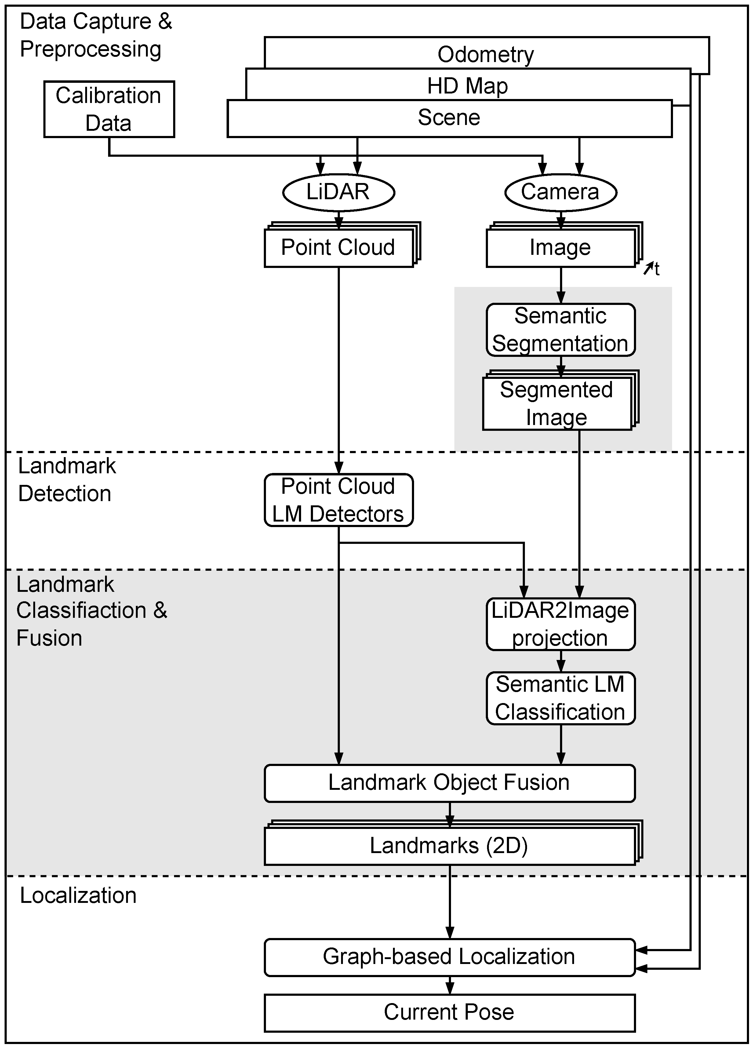
3.1. Methods’ Overview
Figure 1 shows the information flow in the localization system. We used the graph-based method for vehicle self-localization from [
12] as a baseline method. In
Figure 1, the baseline method is presented on the left side. Only LiDAR information is used to detect landmarks based on geometry. These landmarks are co-registered within a 2D map.
The right path shows the processing pipeline for landmark classification with the help of camera information and sensor data fusion. The images are semantically segmented with an adapted version of ERFNet [
22]. An exemplary output of the segmentation network is shown in
Figure 2. The colors represent the respective classes and can be seen as a per-pixel classification of the whole image. The same geometry-based detectors as in the baseline method are used, but now, the detections are classified with camera information by projection into the segmented image obtained by the camera. By combining the geometry information from the LiDAR and the class information from the semantic segmentation, a layered classification model was developed. This is presented in
Section 3.2. The semantic landmark classification is further presented in
Section 3.3.
3.2. Layered Landmark Model
Instead of utilizing geometry to determine a landmark’s type, we aim to introduce camera information for landmark classification. Because an a priori HD map is used in the localization procedure, the classification task is split into two parts. Firstly, the information gathered by sensors has to be enhanced by class labels. Furthermore, the HD map must hold the information needed for map matching on a semantic class label.
Most current approaches use a 2D feature map based on geometric shapes. For map matching, this is helpful to reduce run-time, whereas it is not sufficient for projection to camera images, because the height information is missing. In this work, we use maps in the OpenDrive Format 1.4H with a high variety of different class types and 3D information for certain objects.
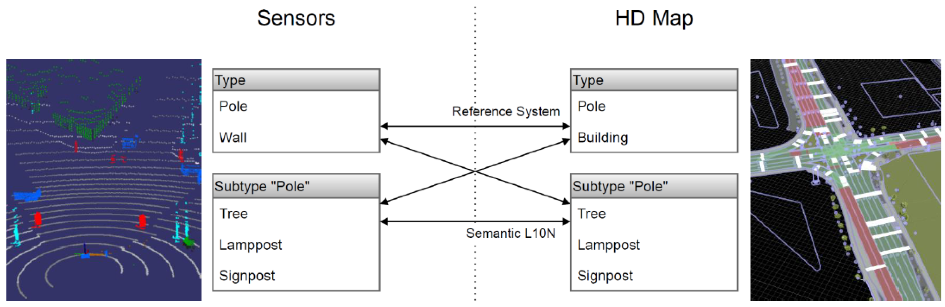
Figure 3 shows the landmark information provided by sensors on the left and information gathered from the HD map on the right. The arrows represent possible map matching configurations. The upper arrow shows the map matching utilized by the baseline model only depending on geometric information. There is no need for further semantic class information on either side. In this case, a pole-like landmark on the sensor side can be matched only with pole-like objects in the map. Without further distinction, a tree could be matched with a sign post of the same radius.
In
Figure 3, the lower boxes represent subtypes of the provided geometric landmark types. All landmark types are extended with subtypes in a layered model. A set of subtypes for the landmark type “Pole” is displayed as an example. On the sensor side, the detected pole can be further classified as vegetation or a traffic sign post with the help of camera information. If the same information also is present in the map, a robust matching of pole-like structures is possible. This means that a tree will only be matched with a tree and a sign post will only be matched with a sign post.
The layered model also enables map matches between different levels of detail on the sensor and map side represented by the diagonal arrows. One possibility is a localization system with semantic information matching against an HD map with only geometric landmark representations. The other possibility is a LiDAR-only localization system using an HD map with extended landmark types. If the sensor system lacks cameras and no classification is performed, a detected “Pole”-type landmark without semantic classification can either be matched to a “Tree” or a “Sign post” subtype marked in the map.
The types and subtypes of the layered landmark model are described in
Table 1. Whereas the main landmark types focus more on geometric information, the subtypes further divide the landmarks into semantic classes of the same geometric type.
3.3. Semantic Object Classification
In prior work [
2], we stated that the avoidance of the misclassification of pedestrians and poles can be achieved by using semantic information. The semantic object classification uses the landmark detectors for poles from [
16] to retrieve the geometric type and then uses camera information to estimate a semantic subtype.
As depicted in the concept overview in
Figure 1, the data used in this method include one LiDAR sample, which consists of a set of points generated from one 360-degree turn of the laser scanner and one camera image. In our case, we focus on the front of our test vehicle, so only the front camera is used for semantic classification. As stated above, an ERFNet implementation is used to perform a semantic segmentation on the image.
The detected pole-like landmarks in the 3D LiDAR point cloud are used to generate 2D bounding boxes in the semantic image. With the information of each landmark’s position, radius, and height, a bounding box is generated in 3D space. With the known calibration parameters of the LiDAR and camera, the 3D bounding box is projected into the camera image. The bounding boxes in the 2D frame determine the pixels in the semantically segmented image used for landmark classification. The label that occurs most frequently in the bounding box defines the subtype of the landmark in addition to the geometric type received from the landmark detection. An exemplary output of the method can be found in
Figure 4.
In this work, we focus on four semantic classes only: pole, pedestrian, vegetation, and else. These types can be differentiated with the used ERFnet segmentation network with pre-trained weights. The method describes the principle, although not all landmark subtypes from
Table 1 are used in this method. Using these four classes already promises several advantages:
Pole-like landmarks are confirmed by the camera, and landmarks that cannot be classified properly (e.g., type Else) can be omitted from the position estimation if sufficient information with a high belief score is present.
Pole-like structures that are not static can be omitted instantaneously. Landmarks classified as Pedestrian will be deleted and not further used.
The distinction between Pole and Vegetation is expected to increase robustness due to fewer false-positive map matches.
Based on the current state of the graph in terms of the number of landmarks, map matches, and the current estimated relative accuracy, landmarks are processed slightly differently. The more landmarks are available, correctly matched, and have a strong belief score, and the fewer new measurements need to be added to the graph to maintain a good accuracy. The threshold for adding landmarks to the graph will therefore be adjusted at runtime, and subtype-classified landmarks will be preferred over geometry-based measurements. This not only decreases complexity, but also the run-time of the optimization algorithm.
3.4. Metrics of Robustness
The International Standard for Systems and Software Engineering defines robustness as “the degree to which a system or component can function correctly in the presence of invalid inputs or stressful environmental conditions” [
40]. Based on this definition and the inputs from [
27,
28] as described in
Section 2, a specific robustness definition approach for localization systems is defined. The three key indicators, namely “correct function”, “invalid inputs”, and “stressful environmental conditions”, serve as the basis of the robustness evaluation in this work.
As stated by [
9], the localization problem is split into two parts. Firstly, landmarks are detected in a localization front end. The front end processes raw sensor inputs and, so, is dependent on the sensor type. The detected landmarks are then provided to the sensor-agnostic localization back end to estimate the current pose. Based on this system definition, the three indicators will be applied to the localization system under test as black box model:
- (a)
The subsystem detection;
- (b)
The subsystem matching;
- (c)
The localization system as a whole.
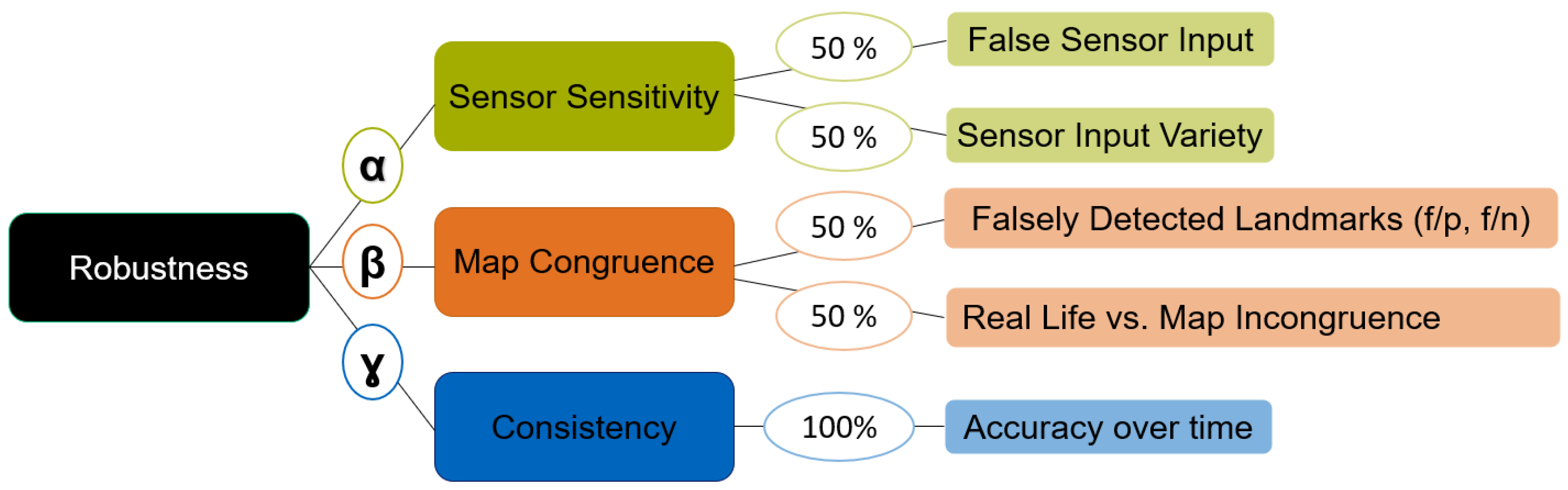
This leads to the three pillars of the robustness of landmark-based localization systems, also depicted in
Figure 5:
Sensor sensitivity: Only the detection subsystem is provided with the raw sensor data. The subsequent matching subsystem, being provided with detected landmarks and thus without a direct link to the sensor input, can be considered sensor-agnostic. Sensor sensitivity therefore evaluates the performance of the detection system and is used to evaluate its robustness against false or noisy sensor input and the variety of different input sensor types.
Map congruence: The input of the matching subsystem consists of the detected landmarks and a prior recorded map of the environment. The three main sources of potential errors in matching can come from an error in the matching algorithm, an incorrect or deviant input in detected landmarks, or a map error. Our focus is on evaluating the robustness with respect to falsely matched landmarks and incongruence between the real environment and the map.
Consistency: In
Section 1, the overall localization accuracy tolerance for urban autonomous applications was set to
cm in [
1]. The position calculated by the localization system is measured and compared to the position given by the reference system. The absolute error
is then compared to the position tolerance
. Observing the correct function (current pose accuracy within tolerance) of the localization system over multiple consecutive timestamps leads to the term consistency. It is seen as one major pillar contributing to the overall robustness of the localization system.
3.5. Robustness Score
A robustness score for neural network benchmarking was introduced in [
13] and applied to localization benchmarking in this work. To evaluate the robustness to different types of faults, perturbations
p in three degrees of severity
s are applied to the system. For example, Gaussian noise is applied to the GPS data for initialization at different levels. The ability to cope with these input changes is evaluated for different levels, and the influence on the localization tasks is measured, then an error term
is calculated. The full list of perturbations used to calculate the robustness score’s parts can be found in
Section 4.3.
All perturbations are applied one by one to separate their individual influences. Grouping the perturbation types as described in
Section 3.4 leads to the perturbation error (PE) terms:
where the detection and matching performance and localization accuracy with respect to perturbation type and severity are denoted. The robustness score (RS) is then calculated by a weighted sum of all the given error terms.
Figure 5 shows the composition of the different metrics. The parameters
,
, and
are used to weight the influence of the error terms
.
represents the mean variance of all terms
.
and
are defined by the variances for
and
. The values are normalized to sum up to 1 and are defined by evaluating the variances for multiple test drives in different environments.
4. Experiments
Several experiments were performed to evaluate the robustness and the influence of semantic information for vehicle self-localization. Since the localization task can be seen as an open-loop method, the raw input is the same regardless of the localization method. Furthermore, the output will no change the driven path or the sensor positions during a recorded test drive.
For a qualified comparison of the influence on the robustness for different fault injections, a measure for robustness is defined and applied to a set of test drives with different localization parameters. As a baseline system, the graph-based method for vehicle self-localization from [
12] is used. The system robustness is then evaluated with the robustness score from
Section 3.5. Furthermore, the influence of semantic information on the detection and matching performance is examined.
Section 4.1 shows the test vehicle and sensor configuration. The test drives used for robustness evaluations are listed in
Section 4.2.
Section 4.3 gives detailed information on the perturbation injections used to calculate the robustness score for the respective test drives.
4.1. Experimental Setup
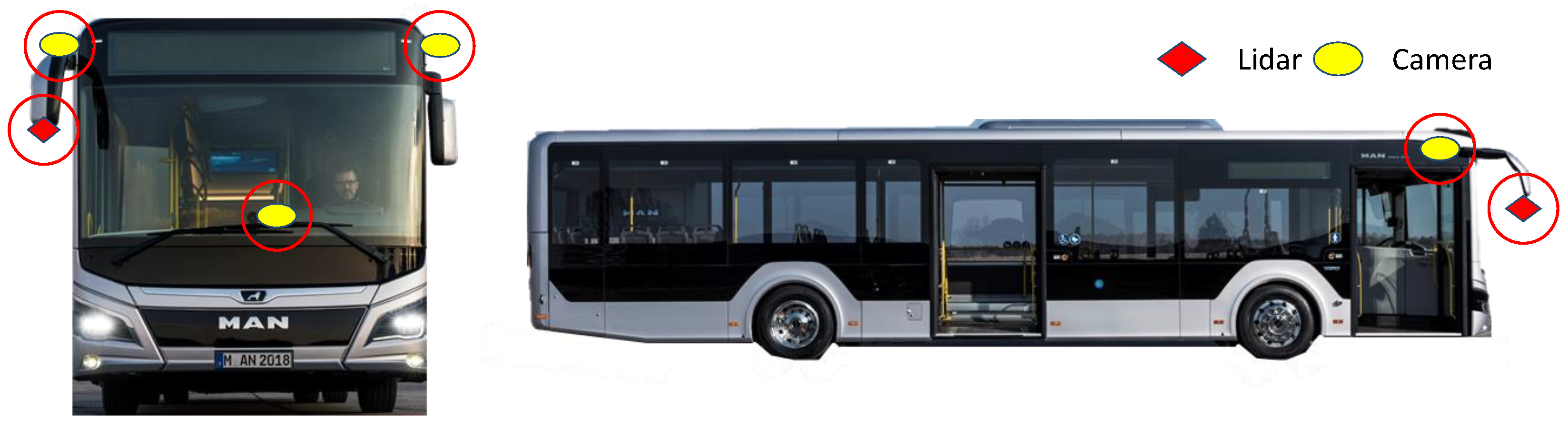
The methods from
Section 3.3 were implemented for real-time use in a 12 m-long MAN Lion’s City bus, which served as a test vehicle. This vehicle is equipped with various sensor types. The main sensors used in this work are a 32-layered rotating laser scanner and cameras with a resolution of 2.3 MP and a horizontal field of view (FOV) of 120°. The mounting positions are shown in
Figure 6. The laser scanner was mounted to the front right of the vehicle to perceive a 270° FOV to the front and right of the bus. Three cameras were mounted facing the front, right, and left. Furthermore, the vehicle is equipped with a real-time kinematic (RTK) system, which consists of a GNSS sensor and acceleration sensors. The algorithms were programmed in C++ and make use of the Point Cloud Library (PCL) and OpenCV. The modules were executed on industrial PCs with an x86 architecture and on an NVIDIA AGX Xavier with an ARM architecture. This system is capable of giving the current pose within a few centimeters and was used as a reference system for our localization.
4.2. Real-World Test Drives
Eight test drives with the test vehicle were selected for comparison. For the evaluation of the generalization performance of the selected methods, different operational design domains (ODDs) were used. Routes in Karlsfeld, Germany, a suburban environment, as well as in the Aldenhoven Testing Center (ATC), Germany, were selected for comparison.
Table 2 shows the ODDs and the detectable landmarks of the respective test drives.
4.3. Perturbation Injections for Robustness Calculation
As proposed by [
9], the localization system under test was divided into two parts. The front end includes landmark detectors and the classification of landmarks. The output is a collection of landmarks that are semantically labeled, if the camera information is available. Otherwise, the landmarks will only be defined by their geometry. The front end’s output is directed to the localization back end, in this case, a graph-based optimization. The back end uses the sensor-agnostic measurements to build up a factor graph and calculate the current pose based on prior measurements and matches against an HD map.
To determine robustness, we injected perturbations into the system at different points. Perturbations were chosen considering possible real-world implications on the environment, sensors, or system. The first set of perturbations is introduced right before the front end. The initial sensor input is altered to evaluate the resilience of the landmark detectors against sensor faults. The modeled sensor faults used in this work were noisy inputs for the odometry estimation and the GNSS signal, as well as random offsets to the odometry signal. Furthermore, the sample rate of the laser scanner was lowered to mimic a lower-priced sensor. The last perturbation injection is a static rotation to the LiDAR sensor to simulate the wrong calibration. Another way to test robustness is to alter the landmarks that were detected by the localization front end before they are provided to the back end. This mainly influences the matching performance within the position estimation. Here, multiple detections were added to the set of found landmarks or random landmarks were deleted, representing false-positive or false-negative measurements, respectively. Another modification is to add an offset to the positions of landmarks or filter landmarks further away from the vehicle than a specific distance. This simulates a foggy or rainy environment. In this work, no distinction between LiDAR and camera measurements is made, and all landmarks detected further away than the given distance were removed. All types of perturbations
p, their applied parameter changes, and the respective values for each of the three levels of severity
s can be found in
Table 3.
All test drives were evaluated with all listed perturbations. The perturbation injections were furthermore performed on the baseline system and the localization with semantic landmark classification separately. Therefore, the influence of perturbation injections can be differentiated from the influence of semantic information on robustness.
5. Results
The robustness of all recorded test drives outlined in
Section 4.2 was evaluated with the novel robustness metric described in
Section 3.4 and
Section 3.5. This section is split into two parts.
Section 5.1 shows the results for the baseline system robustness score in different operational design domains. Here, the focus lies on the evaluation metrics and the evaluation method.
Section 5.2 highlights the impact of semantic information for vehicle self-localization.
5.1. Robustness Evaluation of the Baseline System
The perturbation errors
were calculated for each test drive, each perturbation
p, and severity level
s. The mean value of all errors per perturbation are clustered to the error term
. The error terms for the respective test drives are listed in
Table 4. The baseline system only uses the rotating laser scanner to detect landmarks. The cameras are not used in this step of the work.
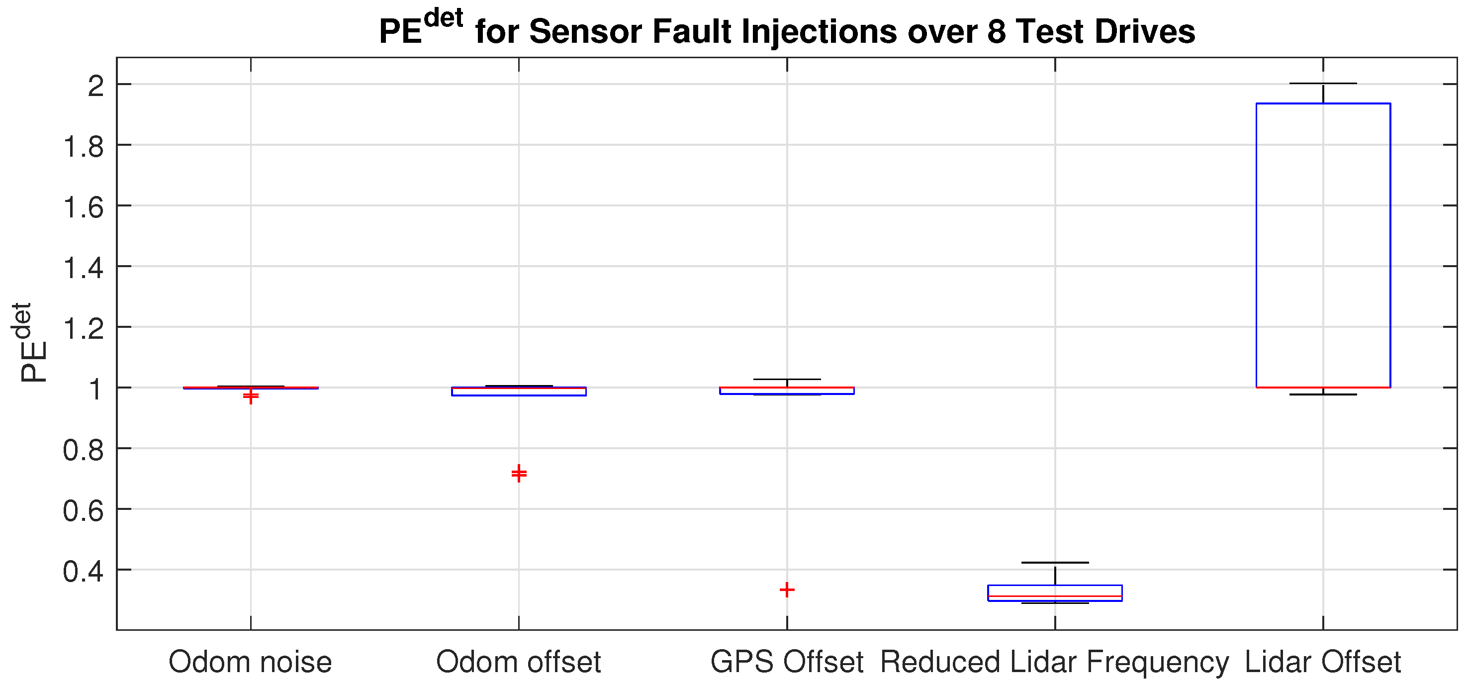
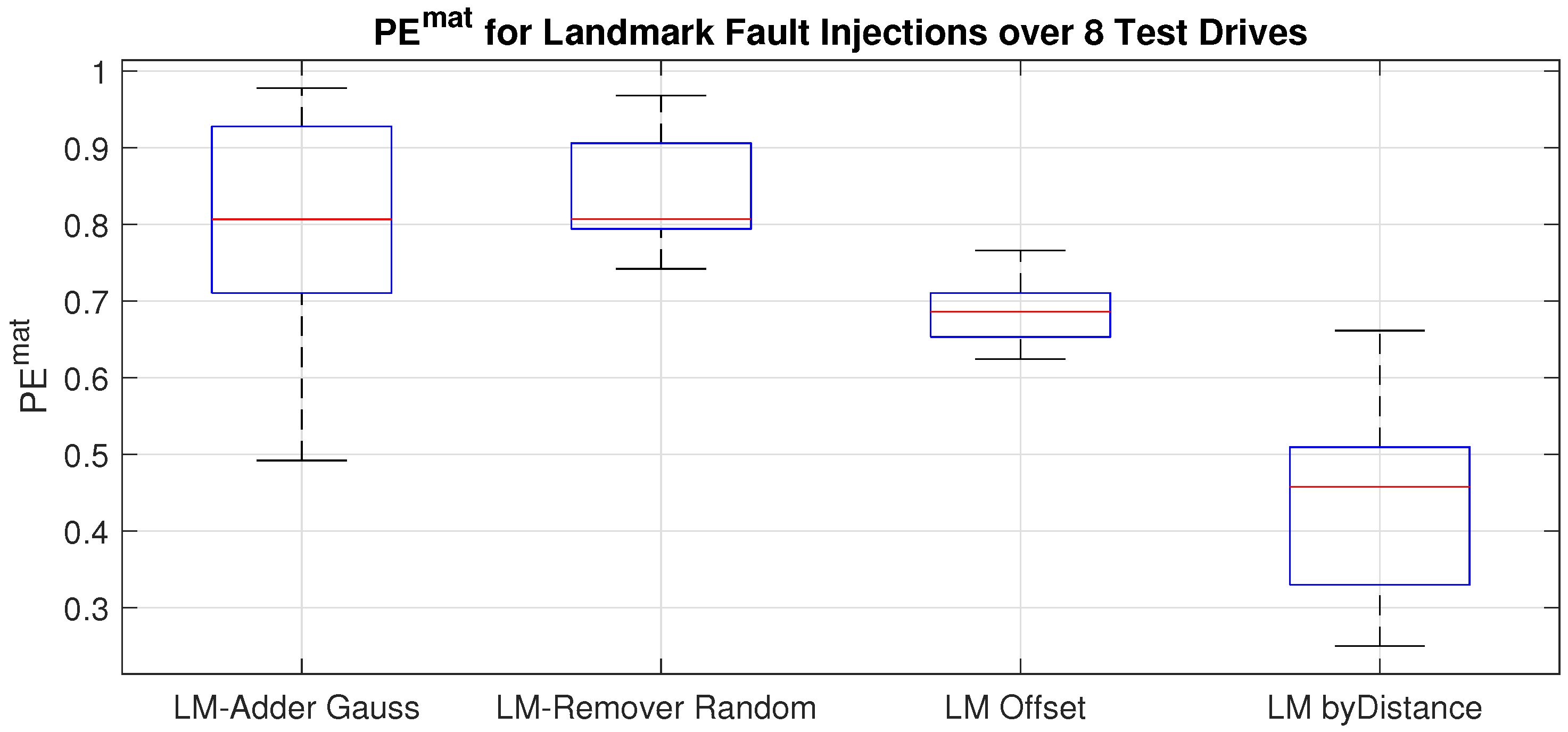
To further investigate the influence of the individual perturbations, the distributions of error terms for detection are displayed in
Figure 7 and for matching the distributions are shown in
Figure 8.
For detection perturbations, the variances for the first four fault injections were within 5%, while the impact of LiDAR offset had a greater influence on the robustness. Although reducing the LiDAR frequency gave similar output in all ODDs, the mean robustness score for detections was reduced to about 40% with respect to unlimited LiDAR frequency.
In contrast to the sensor perturbation errors, all fault injections directly on landmarks resulted in a higher variance on the robustness score for matching. While adding or removing random landmarks still gave high robustness terms between 70% and 90% with respect to the baseline, the robustness decreased by offsetting the detected landmarks or limiting the maximum range where landmarks can be detected. The latter led to a reduction of the matching performance of 30% to 50% and also had the biggest impact on the perturbation error term for matching.
To visualize the reduction of the detection range and its influence on the matching performance, all matched landmarks for Test Drive 02 in Karlsfeld (
Table 2) are presented in
Figure 9 for the respective severity levels. The top left image shows the baseline model as a reference for all detectable pole landmarks. The other images present the three levels of severity for the fault injection where the range was limited to 30 m, 20 m, and 10 m. The number of matched poles decreased with shorter detection ranges.
The robustness scores for the analyzed localization system were calculated according to Equation (
2) over all test drives, as well as clustered to the respective characteristics.
Table 5 shows the perturbation errors for detection, matching, and pose, respectively. In addition to that, the robustness score was calculated for the scenarios of Karlsfeld and Aldenhoven separately to show the influence of their respective ODD. The variances of the clustered error term from
Table 4 define the values for
,
, and
. The value of
was therefore calculated from the variance for “Odometry Noise”, “Odometry Offset”, “GPS Offset”, “LiDAR Downsample”, and “LiDAR Rotational Offset” and then averaged over all test drives. The three values were then normalized and set as follows:
5.2. Robustness Evaluation with Semantic Class Labels
The perturbation injections from
Section 4.3 were performed also on a localization system with the semantic classification of landmarks. For the semantic classification, LiDAR, as well as cameras were used. As this work highlights the semantic classification of pole-like landmarks, only landmarks with geometric type “Pole” were considered. Furthermore, the LiDAR’s field of view was not fully covered by the camera image. Landmarks that were not in the camera image cannot be classified and, therefore, were considered as type “Pole” and subtype “Pole” (
Table 1).
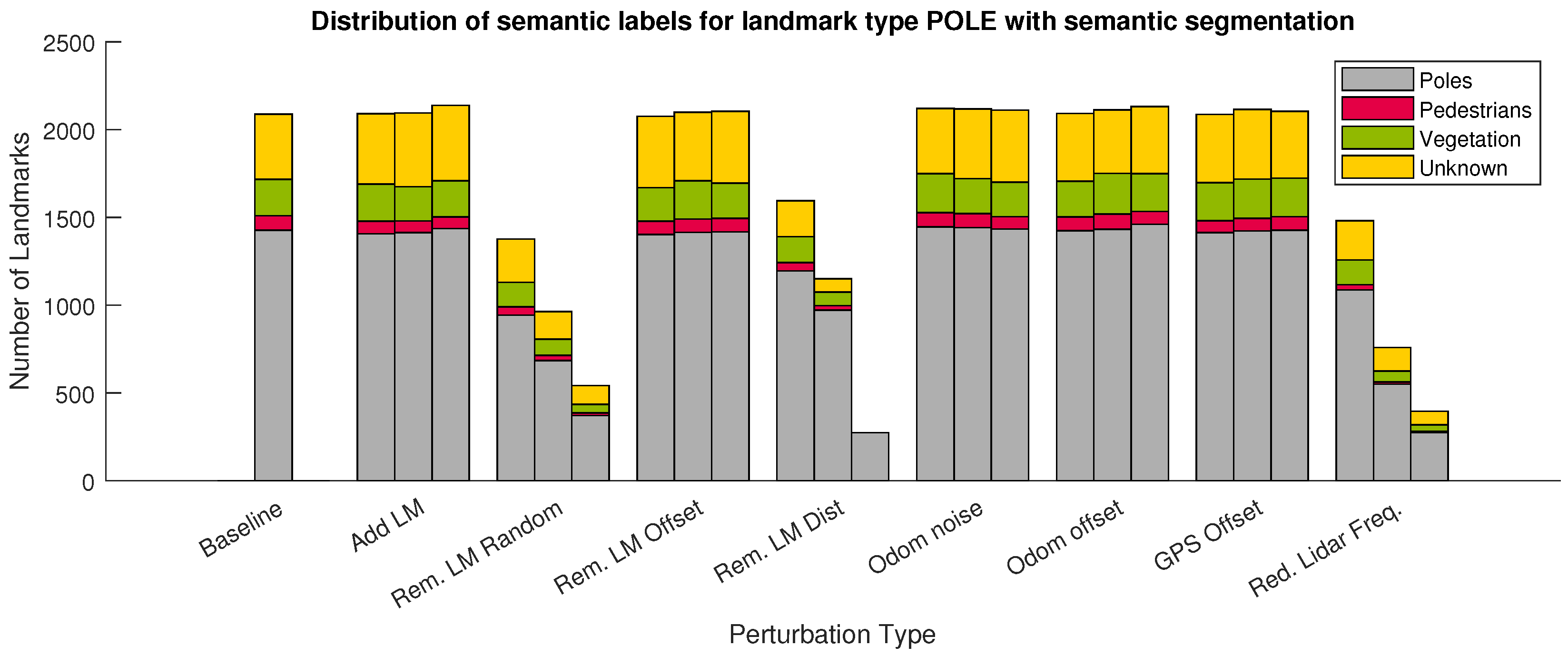
Figure 10 shows the distribution of the subtypes for pole-like landmarks for Test Drive 01 per fault injection. It is clearly seen that the raw number of used landmarks did not change, but the classification can be used to discard non-static landmarks such as pedestrians or landmarks that cannot be confirmed to be actual poles.
Although the number of landmarks can be reduced by only using valid and confirmed landmarks, the impact of perturbations on robustness was similar for the same faults. Reducing LiDAR frequency or limiting the landmark range also reduced the number of landmarks in a similar way as without semantic information.
6. Discussion
All nine perturbations were deployed on all test drives. In
Section 5, we presented the error values for the respective fault injections, as well as their distributions over the different test drives. From the small changes in landmark detections after inserting offsets or Gaussian noise to odometry or the GPS signal, we derived a high resilience of the system under test for these system errors. In contrast to that, changes to the LiDAR inputs had a high influence on the detection performance. Reducing the frequency of the sensor reduced the number of measurements and, therefore, also the number of detections. Defining every landmark detection as a constraint to the current pose, this also led to less confirmations for the pose estimate. The same holds for limiting the range of the sensors. In reality, this might be the case in bad weather situations such as fog or heavy rain.
Figure 8 shows not only that the variance of the fault injection was high, but also the number of successful matches was the lowest. In the baseline system, the LiDAR scanner was the only sensor used, so the impact on the whole system was high. By using redundant sensors or different sensor modalities, the robustness is expected to be higher.
Removing or adding random landmarks reduced the matching robustness of the system. Nevertheless, with a mean value of about 80% of the baseline matching performance, this still provided good results for pose estimation. In a real-world application, landmark detectors are also subject to false-positive and false-negative measurements. Some landmarks cannot be detected, e.g. due to occlusions. On the other hand, temporary objects in construction sites can be detected as landmarks, but these are not marked in a map. The number of these faulty measurements can be reduced by using semantic class labels for the detected landmarks.
The relative impact of perturbation injections stays similar when using the semantic segmentation. Furthermore, here, the reduction of the LiDAR frequency and limiting the landmark detection range led to significantly lower detections. In contrast to the baseline system, 25% of the pole-like landmarks were classified as “Pedestrian”, “Vegetation”, or “Unknown”. “Pedestrian” landmarks were ejected immediately, and landmarks with class “Unknown” were only considered if not enough confirmed poles were present. Another advantage of the semantic labels was that “Vegetation” landmarks were only matched to trees in the map and “Pole” landmarks were matched with road furniture. This led to lower mismatches.
7. Conclusions
In this work, we presented a method to evaluate the robustness of systems for map-based self-localization and a novel robustness score. Different perturbations were injected on sensor inputs and measurements to assess the localization system’s resilience against these influences. The influence of these injections was tested for eight drives in urban areas and on a test track for automated driving.
The separation of the different perturbation injections enabled the identification of system vulnerabilities. Besides finding that limiting the main sensors for landmark detection led to lower detection and matching rates, the evaluated system was resilient to noise or offset on GNSS sensors and vehicle odometry. By adapting the used perturbations to specific use cases, the system can be further investigated based on the users’ needs.
Furthermore, we identified the potential to reduce false-positive rates for landmark detection by using semantic class labels. We presented a method to enhance the detected landmarks with information from semantically segmented camera images to detect and omit dynamic objects such as pedestrians. Observing the matching rates, this led to a lower false-positive rate than without class labels for the landmarks.
With the novel robustness score, it is possible to evaluate a localization framework with or without the use of semantic class information. This work gave a set of perturbation injections to test a LiDAR-based localization framework. In the future, this set can be adapted to other sensors such as radar or ultrasonic, if they are used for localization. This work highlighted test drives in an urban environment and on test tracks. Other ODDs such as motorways may lead to different results for the robustness score. Future work will have to evaluate the influence of the ODD on the values used for the respective perturbations. Furthermore, test drives in non-optimal conditions such as rain, fog, or at night can be used to provide a more general and complete assumption of the localization robustness.
Using semantic information for landmark classification not only increases the robustness of current localization frameworks, it acts as a door opener for robust mapping by increasing the system reliability. Instead of using only geometric features, false landmark candidates can be discarded and will not occur in the updated map. As we already used an HD map as prior information, we did not focus on mapping in this work.
Author Contributions
Conceptualization, C.R.A., S.J. and U.S.; methodology, C.R.A., J.B. and E.H.; software, S.J., C.R.A., J.B. and E.H.; validation, C.R.A. and E.H.; formal analysis, C.R.A. and E.H.; investigation, C.R.A.; resources, C.R.A., J.B. and E.H.; data curation, C.R.A. and S.J.; writing—original draft preparation, C.R.A.; writing—review and editing, C.R.A., J.B., E.H., S.J. and U.S.; visualization, C.R.A., J.B. and E.H.; supervision, S.J. and U.S.; project administration, U.S.; funding acquisition, U.S. All authors have read and agreed to the published version of the manuscript.
Funding
Part of the research was conducted within @CITY-AF (Research Project No. 19 A 1800 3J), funded by the German Federal Ministry for Economic Affairs and Energy (BMWi).
Institutional Review Board Statement
Not applicable.
Informed Consent Statement
Not applicable.
Data Availability Statement
Some or all data or models that support the findings of this study are available from the corresponding author upon reasonable request.
Conflicts of Interest
The authors declare no conflict of interest.
References
- Levinson, J.; Thrun, S. Robust vehicle localization in urban environments using probabilistic maps. In Proceedings of the IEEE International Conference Robotics and Automation (ICRA), Anchorage, AK, USA, 3–7 May 2010; pp. 4372–4378. [Google Scholar] [CrossRef] [Green Version]
- Albrecht, C.; Névir, D.; Hildebrandt, A.C.; Kraus, S.; Stilla, U. Investigation on Misclassification of Pedestrians as Poles by Simulation. In Proceedings of the IEEE Intelligent Vehicles Symposium, Nagoya, Japan, 11–17 July 2021; pp. 804–809. [Google Scholar] [CrossRef]
- Spangenberg, R.; Goehring, D.; Rojas, R. Pole-Based localization for autonomous vehicles in urban scenarios. In Proceedings of the IEEE/RSJ International Conference on Intelligent Robots and Systems (IROS), Daejeon, Korea, 9–14 October 2016; pp. 2161–2166. [Google Scholar] [CrossRef]
- Kampker, A.; Hatzenbuehlerm, J.; Klein, L.; Sefati, M.; Kreiskoether, K.; Gert, D. Concept Study for Vehicle Self-Localization Using Neural Networks for detection of Pole-like Landmarks. In Proceedings of the International Conference on Intelligent Autonomous Systems(IAS), Singapore, 11–15 June 2018; pp. 689–705. [Google Scholar] [CrossRef]
- Weng, L.; Yang, M.; Guo, L.; Wang, B.; Wang, C. Pole-Based Real-Time Localization for Autonomous Driving in Congested Urban Scenarios. In Proceedings of the IEEE International Conference on Real-time Computing and Robotics (RCAR), Kandima, Maldives, 1–5 August 2018; pp. 96–101. [Google Scholar] [CrossRef]
- Hertzberg, J.; Lingemann, K.; Nüchter, A. Mobile Roboter: Eine Einführung aus Sicht der Informatik; Springer: Berlin/Heidelberg, Germany, 2012. [Google Scholar]
- Liu, R.; Wang, J.; Zhang, B. High Definition Map for Automated Driving: Overview and Analysis. J. Navig. 2020, 73, 324–341. [Google Scholar] [CrossRef]
- Sefati, M.; Daum, M.; Sondermann, B.; Kreisköther, K.D.; Kampker, A. Improving vehicle localization using semantic and pole-like landmarks. In Proceedings of the IEEE Intelligent Vehicles Symposium (IV), Los Angeles, CA, USA, 11–14 June 2017; pp. 13–19. [Google Scholar] [CrossRef]
- Grisetti, G.; Kümmerle, R.; Stachniss, C.; Burgard, W. A Tutorial on Graph-Based SLAM. IEEE Intell. Transp. Syst. Mag. 2010, 2, 31–43. [Google Scholar] [CrossRef]
- Thrun, S.; Fox, D.; Burgard, W.; Dellaert, F. Robust Monte Carlo localization for mobile robots. Artif. Intell. 2001, 128, 99–141. [Google Scholar] [CrossRef] [Green Version]
- Steß, M. Ein Verfahren zur Kartierung und Präzisen Lokalisierung mit Klassifizierten Umgebungscharakteristiken der Straßeninfrastruktur für Selbstfahrende Kraftfahrzeuge. Ph.D. Dissertation, Gottfried Wilhelm Leibniz Universität Hannover, Hannover, Germany, 2017. [Google Scholar] [CrossRef]
- Wilbers, D.; Merfels, C.; Stachniss, C. A Comparision of Particle Filter and Graph-based Optimization for Localization with Landmarks in Automated Vehicles. In Proceedings of the IEEE International Conference on Robotic Computing, Naples, Italy, 25–27 February 2019; pp. 220–225. [Google Scholar] [CrossRef]
- Hendrikx, R.; Pauwels, P.; Torta, E.; Bruyninckx, H.P.; van de Molengraft, M. Connecting Semantic Building Information Models and Robotics: An application to 2D LiDAR-based localization. In Proceedings of the IEEE International Conference on Robotics and Automation (ICRA), Xi’an, China, 30 May–5 June 2021; pp. 11654–11660. [Google Scholar] [CrossRef]
- Stachniss, C. Simultaneous Localization and Mapping. In Handbuch der Geodäsie; Freeden, W., Rummel, R., Eds.; Springer Reference Naturwissenschaften, Springer Spektrum: Berlin/Heidelberg, Germany, 2016. [Google Scholar]
- Brenner, C. Global Localization of Vehicles Using Local Pole Patterns. In Pattern Recognition; Springer: Berlin/Heidelberg, Germany, 2009; pp. 61–70. [Google Scholar] [CrossRef]
- Wilbers, D.; Merfels, C.; Stachniss, C. Localization with Sliding Window Factor Graphs on Third-Party Maps for Automated Driving. In Proceedings of the IEEE International Conference on Robotics and Automation (ICRA), Montreal, QC, Canada, 20–24 May 2019; pp. 5951–5957. [Google Scholar] [CrossRef]
- Meyer, G.P.; Laddha, A.; Kee, E.; Vallespi-Gonzalez, C.; Wellington, C.K. Lasernet: An efficient probabilistic 3d object detector for autonomous driving. In Proceedings of the IEEE International Conference on Computer Vision and Pattern Recognition (CVPR), Long Beach, CA, USA, 21–26 July 2019; pp. 12677–12686. [Google Scholar] [CrossRef] [Green Version]
- Dong, H.; Chen, X.; Stachniss, C. Online Range Image-based Pole Extractor for Long-term LiDAR Localization in Urban Environments. In Proceedings of the European Conference on Mobile Robots (ECMR), Bonn, Germany, 31 August–3 September 2021; pp. 1–6. [Google Scholar] [CrossRef]
- Woo, A.; Fidan, B.; Melek, W.W. Localization for Autonomous Driving. In Handbook of Position Location; Zekavat, S.A., Buehrer, R.M., Eds.; IEEE Series on Digital & Mobile Communication; John Wiley & Sons, Ltd.: Hoboken, JY, USA, 2018; pp. 1051–1087. [Google Scholar] [CrossRef]
- Toft, C.; Olsson, C.; Kahl, F. Long-Term 3D Localization and Pose from Semantic Labellings. In Proceedings of the IEEE International Conference on Computer Vision Workshops (ICCVW), Venice, Italy, 22–29 October 2017; pp. 650–659. [Google Scholar] [CrossRef]
- Xie, Y.; Tian, J.; Zhu, X.X. Linking Points with Labels in 3D: A Review of Point Cloud Semantic Segmentation. IEEE Geosci. Remote Sens. Mag. 2020, 8, 38–59. [Google Scholar] [CrossRef] [Green Version]
- Romera, E.; Alvarez, J.M.; Bergasa, L.M.; Arroyo, R. ERFNet: Efficient residual factorized convnet for real-time semantic segmentation. IEEE Trans. Intell. Transp. Syst. 2017, 19, 263–272. [Google Scholar] [CrossRef]
- Badrinarayanan, V.; Kendall, A.; Cipolla, R. SegNet: A Deep Convolutional Encoder-Decoder Architecture for Image Segmentation. IEEE Trans. Pattern Anal. Mach. Intell. 2017, 39, 2481–2495. [Google Scholar] [CrossRef] [PubMed]
- Patel, N.; Krishnamurthy, P.; Khorrami, F. Semantic Segmentation Guided SLAM Using Vision and LIDAR. In Proceedings of the 50th International Symposium on Robotics (ISR 2018), Munich, Germany, 20–21 June 2018; pp. 1–7. [Google Scholar]
- Li, L.; Yang, M.; Wang, B.; Wang, C. An overview on sensor map based localization for automated driving. In Proceedings of the Joint Urban Remote Sensing Event (JURSE), Dubai, United Arab Emirates, 6–8 March 2017; pp. 1–4. [Google Scholar] [CrossRef]
- Wu, C.; Huang, T.A.; Muffert, M.; Schwarz, T.; Gräter, J. Precise Pose Graph Localization with Sparse Point and Lane Features. In Proceedings of the 2017 IEEE/RSJ International Conference on Intelligent Robots and Systems (IROS), Vancouver, BC, Canada, 24–28 September 2017; pp. 4077–4082. [Google Scholar] [CrossRef]
- Cadena, C.; Carlone, L.; Carillo, H.; Latif, Y.; Scaramuzza, D.; Neira, J.; Reid, I.; Leonard, J.J. Past, Present, and Future of Simultaneous Localization and Mapping: Toward the Robust-Perception Age. IEEE Trans. Robot. 2016, 32, 1309–1332. [Google Scholar] [CrossRef] [Green Version]
- Bujanca, M.; Shi, X.; Spear, M.; Zhao, P.; Lennox, B.; Luján, M. Robust SLAM Systems: Are We There Yet? In Proceedings of the IEEE/RSJ International Conference on Intelligent Robots and Systems (IROS), Prague, Czech Republic, 27 September–1 October 2021; pp. 5320–5327. [Google Scholar] [CrossRef]
- Brenner, C. Vehicle Localization Using Landmarks Optained by a LIDAR Mapping System. Int. Arch. Photogramm. Remote Sens. Spatial Inf. Sci. 2010, XXXVIII, 139–144. [Google Scholar] [CrossRef]
- Vysotska, O.; Stachniss, C. Improving SLAM by Exploiting Building Information from Publicly Available Maps and Localization Priors. J. Photogramm. Remote Sens. Geoinf. Sci. 2017, 85, 53–65. [Google Scholar] [CrossRef]
- Berrio, J.S.; Ward, J.; Worrall, S.; Nebot, E. Identifying robust landmarks in feature-based maps. In Proceedings of the IEEE Intelligent Vehicles Symposium, Paris, France, 9–12 June 2019; pp. 1166–1172. [Google Scholar] [CrossRef] [Green Version]
- Yurtsever, E.; Lambert, J.; Carballo, A.; Takeda, K. A Survey of Autonomous Driving: Common Practices and Emerging Technologies. IEEE Access 2020, 8, 58443–58469. [Google Scholar] [CrossRef]
- Xia, Z.; Tang, S. Robust self-localization system based on multi-sensor information fusion in city environments. In Proceedings of the 2019 International Conference on Information Technology and Computer Application (ITCA), Guangzhou, China, 20–22 December 2019; pp. 14–18. [Google Scholar] [CrossRef]
- Geiger, A.; Lenz, P.; Urtasun, R. Are we ready for autonomous driving? The KITTI vision benchmark suite. In Proceedings of the IEEE Conference on Computer Vision and Pattern Recognition (CVPR), Providence, RI, USA, 16–21 June 2012; pp. 3354–3361. [Google Scholar] [CrossRef]
- Everingham, M.; Winn, J. The pascal visual object classes challenge 2012 (voc2012) development kit. Pattern Anal. Stat. Model. Comput. Learn. 2011, 8, 5. [Google Scholar]
- Carlone, L.; Bona, B. A comparative study on robust localization: Fault tolerance and robustness test on probabilistic filters for range-based positioning. In Proceedings of the International Conference on Advanced Robotics (ICAR), Munich, Germany, 22–26 June 2009; pp. 1–8. [Google Scholar]
- Yi, S.; Worrall, S.; Nebot, E. Metrics for the evaluation of localisation robustness. In Proceedings of the IEEE Intelligent Vehicles Symposium (IV), Paris, France, 9–12 June 2019; pp. 1247–1253. [Google Scholar] [CrossRef] [Green Version]
- Rebut, J.; Bursuc, A.; Pérez, P. StyleLess layer: Improving robustness for real-world driving. In Proceedings of the IEEE/RSJ International Conference on Intelligent Robots and Systems (IROS), Prague, Czech Republic, 27 September–1 October 2021; pp. 8992–8999. [Google Scholar] [CrossRef]
- Shekar, A.; Gou, L.; Ren, L.; Wendt, A. Label-Free Robustness Estimation of Object Detection CNNs for Autonomous Driving Applications. Int. J. Comput. Vis. 2021, 129, 1185–1201. [Google Scholar] [CrossRef]
- ISO/IEC/IEEE 24765:2017(E); Systems and Software Engineering—Vocabulary. ISO: Geneva, Switzerland, 2017.
| Publisher’s Note: MDPI stays neutral with regard to jurisdictional claims in published maps and institutional affiliations. |
© 2022 by the authors. Licensee MDPI, Basel, Switzerland. This article is an open access article distributed under the terms and conditions of the Creative Commons Attribution (CC BY) license (https://creativecommons.org/licenses/by/4.0/).


