L₀ and L_p Loss Functions in Model-Robust Estimation of Structural Equation Models

Abstract

The $L_p$ loss function has been used for model-robust estimation of structural equation models based on robustly fitting moments. This article addresses the choice of the tuning parameter $\mathsf{\epsilon }$ that appears in the differentiable approximations of the nondifferentiable $L_p$ loss functions. Moreover, model-robust estimation based on the $L_p$ loss function is compared with a recently proposed differentiable approximation of the $L_0$ loss function and a direct minimization of a smoothed version of the Bayesian information criterion in regularized estimation. It turned out in a simulation study that the $L_0$ loss function slightly outperformed the $L_p$ loss function in terms of bias and root mean square error. Furthermore, standard errors of the model-robust SEM estimators were analytically derived and exhibited satisfactory coverage rates.

1. Introduction

Structural equation models (SEMs) and confirmatory factor analysis (CFA) are important statistical methods for analyzing multivariate data in the social sciences [1,2,3,4,5]. In these models, a multivariate vector $\mathit{X}=(X_1,\dots ,X_I)$ of I continuous observed variables (also referred to as items or indicators) is modeled as a function of a vector of latent variables (i.e., factors or traits) $\mathit{\eta }$. SEMs represent the mean vector $\mathit{\mu }$ and the covariance matrix $\mathrm{\Sigma }$ of the random variable $\mathit{X}$ as a function of an unknown parameter vector $\mathit{\theta }$. In SEMs, constrained estimation of the moment structure of the multivariate normal distribution is applied [6].

The measurement model in an SEM is given as

$$\mathit{X}=\mathbf{\nu }+\mathrm{\Lambda }\mathit{\eta }+\mathit{ϵ}.$$

(1)

We denote the covariance matrix $\mathsf{Var}\left(\mathit{ϵ}\right)=\mathrm{\Psi }$. The vectors $\mathit{\eta }$ and $\mathit{ϵ}$ are multivariate normally distributed. In addition, $\mathit{\eta }$ and $\mathit{ϵ}$ are uncorrelated random vectors. In CFA, the multivariate normal (MVN) distribution is represented as $\mathit{\eta }\sim \mathsf{MVN}(\mathbf{\alpha },\mathrm{\Phi })$ and $\mathit{ϵ}\sim \mathsf{MVN}(\mathbf{0},\mathrm{\Psi })$. Hence, one can represent the mean and the covariance matrix in CFA as

$$\mathit{\mu }\left(\mathit{\theta }\right)=\mathbf{\nu }+\mathrm{\Lambda }\mathbf{\alpha }\mathrm{and}\mathrm{\Sigma }\left(\mathit{\theta }\right)=\mathrm{\Lambda }\mathrm{\Phi }{\mathrm{\Lambda }}^{\top }+\mathrm{\Psi }.$$

(2)

In SEM, a matrix $\mathit{B}$ of regression coefficients can additionally be specified such that

$$\mathit{\eta }=\mathit{B}\mathit{\eta }+\mathbf{\xi }\mathrm{with}\mathsf{E}\left(\mathbf{\xi }\right)=\mathbf{\alpha }\mathrm{and}\mathsf{Var}\left(\mathbf{\xi }\right)=\mathrm{\Phi }.$$

(3)

Hence, the mean vector and the covariance matrix are represented in SEM as

$$\mathit{\mu }\left(\mathit{\theta }\right)=\mathbf{\nu }+\mathrm{\Lambda }{(\mathrm{I}-\mathit{B})}^{-1}\mathbf{\alpha }\mathrm{and}\mathrm{\Sigma }\left(\mathit{\theta }\right)=\mathrm{\Lambda }{(\mathrm{I}-\mathit{B})}^{-1}\mathrm{\Phi }{\left[{(\mathrm{I}-\mathit{B})}^{-1}\right]}^{\top }{\mathrm{\Lambda }}^{\top }+\mathrm{\Psi },$$

(4)

where $\mathrm{I}$ is the identity matrix.

Researchers often parsimoniously parameterize the mean vector and the covariance matrix using a parameter $\mathit{\theta }$ as a summary in an SEM. The model assumptions in SEMs are, at best, merely an approximation of a true data-generating model. In SEMs, model deviations (i.e., model errors) in covariances emerge as a difference between a population covariance matrix $\mathrm{\Sigma }$ and a model-implied covariance matrix $\mathrm{\Sigma }\left(\mathit{\theta }\right)$ (see [7,8,9]). Simultaneously, model errors in the mean vector cause a difference between the population mean vector $\mathit{\mu }$ and the model-implied mean vector $\mathit{\mu }\left(\mathit{\theta }\right)$. As a result, the SEM is misspecified at the population level. It should be noted that the model errors are defined at the population level in infinite sample sizes. In real-data applications with limited sample sizes, the empirical covariance matrix $\mathit{S}$ estimates the population covariance matrix $\mathrm{\Sigma }$, while the mean vector $\overline{\mathit{x}}$ estimates the population mean vector $\mathit{\mu }$.

In this work, estimators with some resistance to model deviations are investigated. In more depth, the presence of some amount of model errors should have no impact on the parameter estimate $\mathit{\theta }$. This robustness property is denoted as model robustness, and it adheres to robust statistics principles [10,11,12]. Model errors in SEMs appear as residuals in the modeled mean vector and the modeled covariance matrix, whereas in traditional robust statistics, observations (i.e., cases or subjects) do not obey an imposed statistical model and should be considered as outliers. That is, an estimator in an SEM should automatically recognize large deviations in $\mathit{\mu }-\mathit{\mu }\left(\mathit{\theta }\right)$ and $\mathrm{\Sigma }-\mathrm{\Sigma }\left(\mathit{\theta }\right)$ as outliers that should not significantly damage the estimated parameter $\mathit{\theta }$.

In previous research, the $L_p$ loss function has been used for model-robust estimation based on moments [13,14]. Non-robust estimators such as maximum likelihood or unweighted and weighted least square estimates will typically result in biased estimates in the presence of model error [14]. In this article, we more thoroughly discuss the choice of the tuning parameter $\mathsf{\epsilon }$ in differentiable approximations of the nondifferentiable $L_p$ loss functions. Furthermore, we compare the $L_p$ loss function with a recently proposed differentiable approximation of the $L_0$ loss function and a direct minimization of a smoothed version of the Bayesian information criterion [15] in regularized estimation. Notable, the $L_0$ loss function minimizes the number of model deviations in a fitted model. If only a few entries in the modeled mean vector (or mean vectors) or covariance matrix (or covariance matrices) deviate from zero at the population level, while all other entries equal zero, the $L_0$ loss function would be the most appropriate fit function. In contrast, if all model deviations differ from zero and unsystematically fluctuate around zero, the $L_p$ or $L_0$ loss functions with $p\le 1$ would be less appropriate. Finally, standard errors for the proposed model-robust estimators based on the delta method are derived in this article. Their performance is assessed by evaluating coverage rates.

To sum up, this article focuses on implementation details of SEM estimation based on the $L_p$ ($0<p\le 1$) and the newly proposed $L_0$ loss functions, while [16] was devoted to regularized SEM estimation, which can also be utilized for model-robust estimation. A comparison of regularized estimation and robust loss functions can be found in [14].

The remainder of the article is organized as follows. Model-robust SEM estimation based on the robust $L_0$ and $L_p$ loss functions is treated in Section 2. Section 3 introduces direct BIC minimization as a special approach to regularized maximum likelihood estimation. Section 4 is devoted to details of standard error computation. In Section 5, research questions are formulated that are addressed in two subsequent simulation studies. In Section 6, bias and root mean square error of model-robust SEM estimators are of interest. Section 7 reports findings regarding the standard error estimation regarding coverage rates. Finally, the article closes with a discussion in Section 8.

2. ${\mathit{L}}_{\mathit{0}}$ and ${\mathit{L}}_{\mathit{p}}$ Loss Functions in SEM Estimation

We now describe model-robust moment estimation of multiple-group SEMs. The treatment closely follows previous work in Refs. [14,16].

The empirical mean vector $\overline{\mathit{x}}$ and the empirical covariance matrix $\mathit{S}$ are sufficient statistics for estimating $\mathit{\mu }$ and $\mathrm{\Sigma }$ when modeling multivariate normally distributed data with no missing values. In particular, they are also sufficient statistics of $\mathit{\mu }\left(\mathit{\theta }\right)$ and $\mathrm{\Sigma }\left(\mathit{\theta }\right)$ that are constrained functions of a parameter vector $\mathit{\theta }$. Hence, $\overline{\mathit{x}}$ and $\mathit{S}$ are also sufficient statistics for the parameter vector $\mathit{\theta }=({\theta }_1,\dots ,{\theta }_K)$ that contains K elements.

Now, assume that there are G groups with sample sizes $N_g$, mean vectors ${\overline{\mathit{x}}}_g$, and covariance matrices ${\mathit{S}}_g$ ($g=1,\dots ,G$). Let ${\mathbf{\xi }}_g=\left({\overline{x}}_g,\mathrm{vech}\left({\mathit{S}}_g\right)\right)$ be the vector of sufficient statistics in group g, where $\mathrm{vech}$ denotes the operator that stacks all nonredundant matrix entries on top of one another. Furthermore, the vector $\mathbf{\xi }=({\mathbf{\xi }}_1,\dots ,{\mathbf{\xi }}_G)$ contains the sufficient statistics of all G groups.

The population mean vectors and covariance matrices are denoted by ${\mathit{\mu }}_g$ and ${\mathrm{\Sigma }}_g$, respectively. The model-implied mean vectors and covariance matrices are denoted by ${\mathit{\mu }}_g\left(\mathit{\theta }\right)$ and ${\mathrm{\Sigma }}_g\left(\mathit{\theta }\right)$, respectively. It is worth noting that the parameter vector $\mathit{\theta }$ lacks an index g, indicating that there can be common and unique parameters across groups. Equal factor loadings and item intercepts across groups are frequently imposed in a multiple-group CFA (i.e., measurement invariance is specified [17,18]).

In model-robust SEM estimation discussed in this article, discrepancies ${\overline{\mathit{x}}}_g-{\mathit{\mu }}_g\left(\mathit{\theta }\right)$ and $\mathrm{vech}\left({\mathit{S}}_g\right)-\mathrm{vech}\left({\mathrm{\Sigma }}_g\left(\mathit{\theta }\right)\right)$ are minimized according to a loss function $\mathsf{\rho }$. There are two kinds of errors that are only, for simplicity, discussed for the mean structure. We can express the discrepancy in the mean structure as

$${\overline{\mathit{x}}}_g-{\mathit{\mu }}_g\left(\mathit{\theta }\right)=\left\{{\overline{\mathit{x}}}_g-{\mathit{\mu }}_g\right\}+\left\{{\mathit{\mu }}_g-{\mathit{\mu }}_g\left(\mathit{\theta }\right)\right\}.$$

(5)

The first term ${\overline{\mathit{x}}}_g-{\mathit{\mu }}_g$ describes a discrepancy due to sampling variation (i.e., with respect to the sampling of subjects). This term can typically be reduced when larger samples are drawn. The second term ${\mathit{\mu }}_g-{\mathit{\mu }}_g\left(\mathit{\theta }\right)$ indicates a model error. This term exists at the population level and, therefore, does not vanish with increasing sample sizes. In model-robust estimation, a few entries in the model error are allowed to differ from zero (i.e., a sparsity assumption), corresponding to model misspecification. Note that the sparsity assumption is vital for the performance of model-robust estimators.

In robust moment estimation, the following fit function $F_{\mathrm{rob}}$ is minimized:

$$F_{\mathrm{rob}}(\mathit{\theta };\mathbf{\xi })=\sum _{g=1}^G\sum _{i=1}^I{w}_{1g,i}\mathsf{\rho }\left({\overline{x}}_{g,i}-{\mu }_{g,i}\left(\mathit{\theta }\right)\right)+\sum _{g=1}^G\sum _{i=1}^I\sum _{j=i}^I{w}_{2g,ij}\mathsf{\rho }\left(s_{g,ij}-{\sigma }_{g,ij}\left(\mathit{\theta }\right)\right).$$

(6)

In the first term at the right side of the equation in (6), discrepancies in the sample means ${\overline{x}}_{g,i}$ from the model-implied mean ${\mu }_{g,i}\left(\mathit{\theta }\right)$ for item i in group g are considered. In the second term at the right side of the equation in (6), discrepancies in the sample covariances $s_{g,ij}$ from the model-implied covariance ${\sigma }_{g,ij}\left(\mathit{\theta }\right)$ for items i and j in group g are considered. The weights $w_{1g,i}$ ($i=1,\dots ,I$) and $w_{2g,ij}$ ($i,j=1,\dots ,I$) are known but can be set to one if all variables have (approximately) the same standard deviation in the sample comprising all groups or the original scaling of the variables reflects the intended weighing of sampling and model errors. The loss function $\mathsf{\rho }$ in (6) should be chosen such that it is resistant to outlying effects in the mean and the covariance structure.

The robust mean absolute deviation (MAD) loss function $\mathsf{\rho }\left(x\right)=\left|x\right|$ was examined in [19,20]. When compared to usually employed SEM estimation approaches, this fit function is more robust to a few model violations, such as unmodeled item intercepts or unmodeled residual correlations of residuals (see [7]).

In this article, we investigate the $L_p$ loss function

$$\mathsf{\rho }\left(x\right)={\left|x\right|}^p\mathrm{for}p>0.$$

(7)

It has been shown that $p<1$ provides more efficient model-robust estimates than $p=1$ (see [7,13]). The $L_p$ loss function with $p=2$ is the square loss function $\mathsf{\rho }\left(x\right)=x^2$ and corresponds to unweighted least squares (ULSs) estimation. However, this loss function does not possess the model robustness property [7]. The $L_p$ loss function $\mathsf{\rho }\left(x\right)=\sqrt{\left|x\right|}={\left|x\right|}^{0.5}$ (i.e., $p=0.5$) is implemented in invariance alignment [21,22,23] and penalized structural equation modeling [24] in the popular Mplus software (Version 8.10., https://www.statmodel.com/support/index.shtml (accessed on 25 September 2023)). The critical aspect of the $L_p$ loss function $\mathsf{\rho }$ defined in (7) is that it is a nondifferentiable function. Consequently, the fit function $F_{\mathrm{rob}}$ in (6) is also nondifferentiable, which does not allow the application of general-purpose optimizers that rely on the differentiable optimization functions. As a remedy, the nondifferentiable $L_p$ loss function $\mathsf{\rho }$ can be replaced by a differentiable approximation ${\mathsf{\rho }}_{\mathsf{\epsilon }}$, which is close to $\mathsf{\rho }$, but differentiable on the entire real line. The approximating function ${\mathsf{\rho }}_{\mathsf{\epsilon }}$ is defined as

$${\mathsf{\rho }}_{\mathsf{\epsilon }}\left(x\right)={\left(x^2+\mathsf{\epsilon }\right)}^{p/2},$$

(8)

where $\mathsf{\epsilon }>0$ is a tuning parameter that should be small enough such that ${\mathsf{\rho }}_{\mathsf{\epsilon }}$ is close to $\mathsf{\rho }$ but large enough to ensure estimation stability. Replacing the nondifferentiable $\mathsf{\rho }$ by the differentiable approximation ${\mathsf{\rho }}_{\mathsf{\epsilon }}$ has been previously recommended by [13,21,25,26].

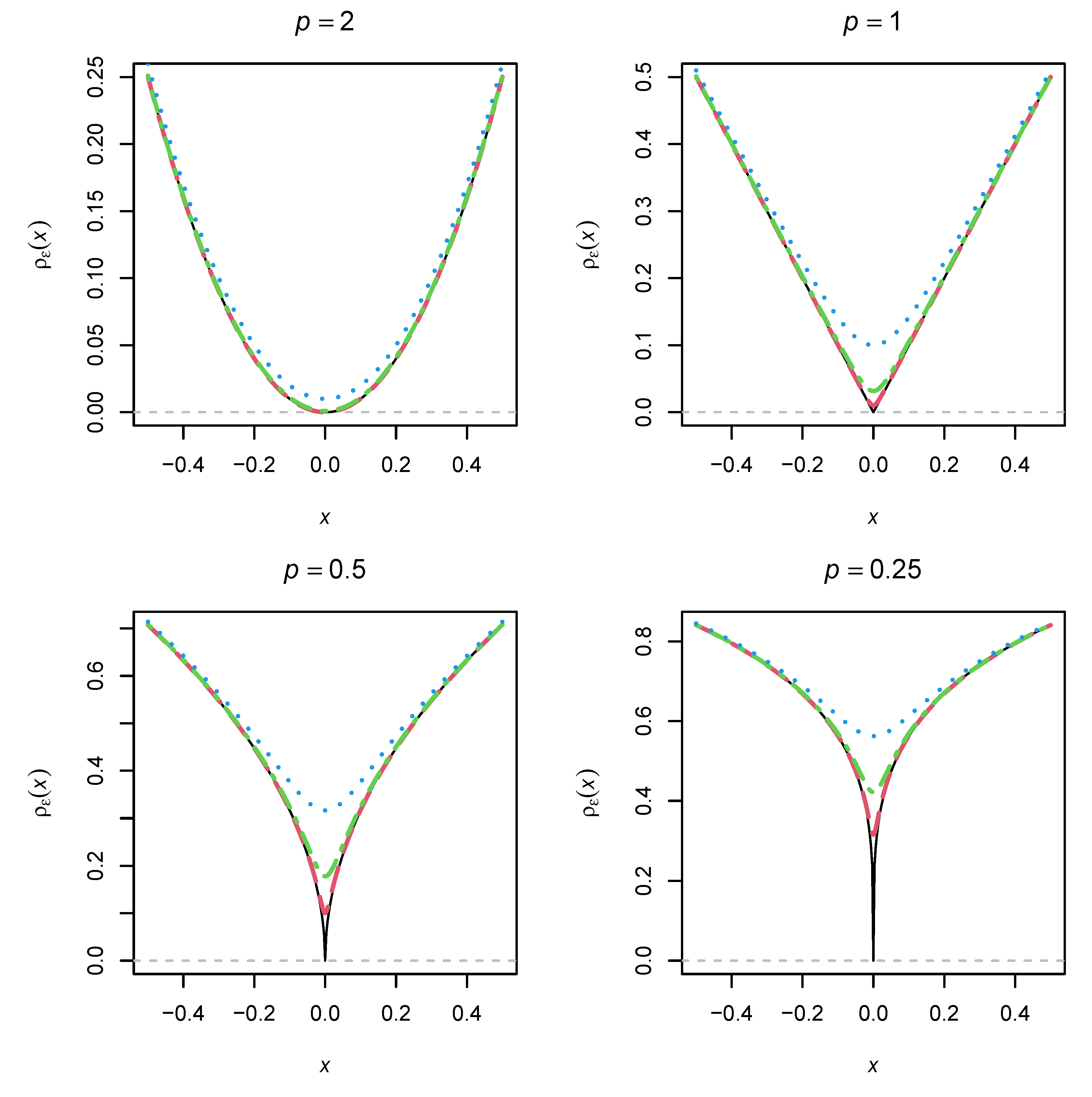
The loss function $\mathsf{\rho }$ and its differentiable approximation ${\mathsf{\rho }}_{\mathsf{\epsilon }}$ are displayed for six different values of p in Figure 1. It can be seen (and shown) that $\mathsf{\rho }\left(x\right)\le {\mathsf{\rho }}_{\mathsf{\epsilon }}\left(x\right)$ for all $p>0$ and $\mathsf{\epsilon }>0$. Furthermore, the loss function $\mathsf{\rho }$ is much steeper at $x=0$ for a smaller p. With a larger $\mathsf{\epsilon }$, the approximation ${\mathsf{\rho }}_{\mathsf{\epsilon }}$ becomes smoother. Choosing an appropriate tuning parameter $\mathsf{\epsilon }>0$ is therefore important when applying model-robust moment estimation based on the $L_p$ loss function.

It might be tempting to use a very small p close to zero. Such a loss function is close to the $L_0$ loss function, which takes the value of 1 for all arguments differently from $x=0$ and 0 for $x=0$. If the sparsity assumption of model errors holds, the $L_0$ would theoretically be the most desirable loss function [27,28]. However, as shown in Figure 1, ${\mathsf{\rho }}_{\mathsf{\epsilon }}$ for $p=0.01$ does not have a clear minimum zero, making this differentiable loss function difficult to apply in practical optimization.

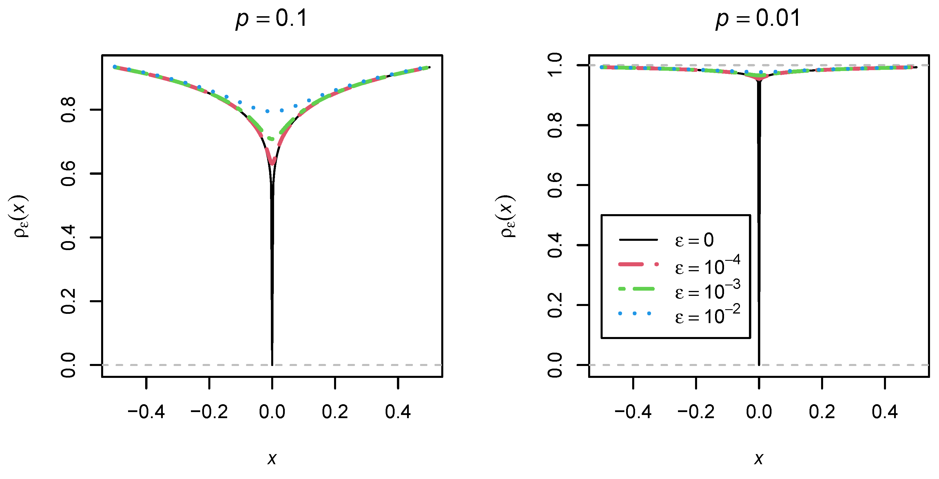
O’Neill and Burke [15,29] proposed the following differentiable approximation ${\mathsf{\chi }}_{\mathsf{\epsilon }}$ of the $L_0$ loss function in a recent work related to regularized estimation:

$${\mathsf{\chi }}_{\mathsf{\epsilon }}\left(x\right)=\frac{x^2}{x^2+\mathsf{\epsilon }},$$

(9)

where $\mathsf{\epsilon }>0$ is again a tuning parameter. The differentiable approximation ${\mathsf{\chi }}_{\mathsf{\epsilon }}$ is displayed for different $\mathsf{\epsilon }$ values in Figure 2. It can be seen that the functional form of ${\mathsf{\chi }}_{\mathsf{\epsilon }}$ seems much nicer to use in optimization than ${\mathsf{\rho }}_{\mathsf{\epsilon }}$ with a p close to 0. Hence, ${\mathsf{\chi }}_{\mathsf{\epsilon }}$ might be a useful alternative robust loss function whose performance in the presence of model errors has to be evaluated.

In practical minimization of $F_{\mathrm{rob}}$ in (6), when $\mathsf{\rho }$ is replaced with ${\mathsf{\rho }}_{\mathsf{\epsilon }}$ (using an appropriate p) or ${\mathsf{\chi }}_{\mathsf{\epsilon }}$, it is advisable to use reasonable starting values and to minimize $F_{\mathrm{rob}}$ using a sequence of differentiable approximations ${\mathsf{\rho }}_{\mathsf{\epsilon }}$ with decreasing $\mathsf{\epsilon }$ values (i.e., subsequently fitting ${\tilde{\mathsf{\rho }}}_{\mathsf{\epsilon }}$ with $\mathsf{\epsilon }={10}^{-1},{10}^{-2},{10}^{-3},{10}^{-4}$, while using the previously obtained parameter estimate as the initial value for the subsequent minimization problem).

3. A Direct BIC Minimization in Regularized Maximum Likelihood Estimation

Most frequently, SEMs are estimated with maximum likelihood (ML) estimation. This estimation method provides the most efficient estimates for correctly specified models. However, the efficiency properties are lost in the case of misspecified SEMs.

As an alternative, regularized ML estimation can be used that introduces an overidentified SEM by allowing free group-specific item intercepts and residual covariances. To identify the model, a penalty function on the overidentified parameters is imposed that is targeted at the sparsity structure of model errors. The methodological literature has extensively documented the regularized estimation of single-group and multiple-group SEMs [30,31,32,33]. Cross-loadings, residual covariances, or item intercepts are regularized in these applications. Regularized SEM estimation enables flexible yet parsimonious model specifications.

In ML estimation, the fit function $F_{\mathrm{ML}}$ is the negative log-likelihood function based on the multivariate normal distribution that is defined as [2,4]

$$F_{\mathrm{ML}}(\mathit{\theta };\mathbf{\xi })=\sum _{g=1}^G\frac{N_g}{2}\left(-Ilog\left(2\pi \right)+\log |{\mathsf{\Sigma }}_g\left(\mathit{\theta }\right)|+\mathrm{tr}\left({\mathit{S}}_g{\mathsf{\Sigma }}_g{\left(\mathit{\theta }\right)}^{-1}\right)+{({\overline{\mathit{x}}}_g-{\mathit{\mu }}_g\left(\mathit{\theta }\right))}^{\top }{\mathsf{\Sigma }}_g{\left(\mathit{\theta }\right)}^{-1}({\overline{\mathit{x}}}_g-{\mathit{\mu }}_g\left(\mathit{\theta }\right))\right).$$

(10)

In empirical applications, the model-implied mean vectors ${\mathit{\mu }}_g$ and covariance matrices ${\mathrm{\Sigma }}_g$ will often be misspecified [34,35,36], and $\mathit{\theta }$ can be understood as a pseudo-true parameter that is defined as the minimizer of $F_{\mathrm{ML}}$ in (10).

In regularized SEM estimation, a penalty function $\mathcal{P}$ is added to the log-likelihood fit function $F_{\mathrm{ML}}$ that imposes some sparsity assumption on a subset of model parameters [31,33]. In order to enforce sparsity, the penalty function $\mathcal{P}$ is often chosen to be nondifferentiable. Define a known parameter ${\iota }_k\in \{0,1\}$ for all parameters ${\theta }_k$, where ${\iota }_k=1$ indicates that for the kth entry ${\theta }_k$ in $\mathit{\theta }$ a penalty function is applied. The penalized log-likelihood function is defined as

$$F_{\mathrm{pen}}(\mathit{\theta },\lambda ;\mathbf{\xi })=F_{\mathrm{ML}}(\mathit{\theta };\mathbf{\xi })+N^{\ast }\sum _{k=1}^K{\iota }_k\mathcal{P}\left(\right|{\theta }_k|,\lambda ),$$

(11)

where $\lambda >0$ is a regularization parameter, and $N^{\ast }$ is a scaling factor that frequently equals the total sample size $N={\sum }_{g=1}^G{N}_g$. The regularized (or penalized) ML estimate is defined as the minimizer of $F_{\mathrm{pen}}(\mathit{\theta };\mathbf{\xi })$.

The least absolute shrinkage and selection operator (LASSO; ref. [37]) or the smoothly clipped absolute deviation (SCAD; ref. [38]) penalty functions have been frequently used in regularized SEM estimation. For a fixed value of $\lambda$, a subset of ${\theta }_k$ parameters for which the penalty function is applied (i.e., ${\iota }_k=1$) will result in estimates of zero. That is, a sparse $\mathit{\theta }$ vector is obtained as the result of regularized estimation. However, the estimate of $\mathit{\theta }$ depends on the fixed regularization parameter $\lambda$; that is,

$$\tilde{\mathit{\theta }}\left(\lambda \right)=\underset{\mathit{\theta }}{arg\; min}{F}_{\mathrm{pen}}(\mathit{\theta },\lambda ;\mathbf{\xi }).$$

(12)

As a result, the parameter estimate $\tilde{\mathit{\theta }}\left(\lambda \right)$ of $\mathit{\theta }$ depends on the unknown parameter $\lambda$. To avoid this problem, the regularized SEM can be repeatedly estimated on a finite grid of regularization parameters $\lambda$ (e.g., on an equidistant grid between 0.01 and 1.00 with increments of 0.01). The Bayesian information criterion (BIC), defined by $\mathrm{BIC}=2F_{\mathrm{ML}}(\mathit{\theta },\mathbf{\xi })+log\left(N\right)H$ may be used to choose an optimal regularization parameter $\lambda$, where H denotes the number of parameters. Because the minimization of BIC is equivalent to the minimization of BIC/2, the final parameter estimate $\widehat{\mathit{\theta }}$ is determined as

$$\widehat{\mathit{\theta }}=\tilde{\mathit{\theta }}\left(\widehat{\lambda }\right)\mathrm{with}\widehat{\lambda }=\underset{\lambda }{arg\; min}\left\{F_{\mathrm{ML}}(\tilde{\mathit{\theta }}\left(\lambda \right),\mathbf{\xi })+\frac{log\left(N\right)}{2}\left(\sum _{k=1}^K{\iota }_k\mathsf{\chi }\left({\tilde{\theta }}_k\left(\lambda \right)\right)\right)\right\},$$

(13)

where the function $\mathsf{\chi }$ is an indicator whether $\left|x\right|$ is different from 0:

$$\mathsf{\chi }\left(x\right)=\left\{\begin{array}{cc}1\hfill & \mathrm{if}\left|x\right|\ne 0\hfill \\ 0\hfill & \mathrm{if}\left|x\right|=0\hfill \end{array}\right.$$

(14)

In particular, the quantity ${\sum }_{k=1}^K{\iota }_k\mathsf{\chi }\left({\tilde{\theta }}_k\left(\lambda \right)\right)$ in (13) counts the number of parameter estimates ${\tilde{\theta }}_k\left(\lambda \right)$ for $k=1,\dots ,K$ for which the penalty function is applied (i.e., ${\iota }_k=1$) and differs from 0.

As becomes clear, regularization SEM estimation necessitates fitting an SEM on a grid of the regularization parameter $\lambda$. This approach is computationally intensive, especially for SEMs with a large number of parameters. The final parameter estimate is obtained by minimizing the BIC across all estimated regularized SEMs. A naïve idea might be directly minimizing the BIC to avoid repeated estimation that involves regularization parameter selection. It should be noted that only a subset of parameters for which sparsity should be imposed is relevant in the BIC computation. Hence, a parameter estimate $\widehat{\mathit{\theta }}$ by minimizing the BIC is provided by

$$\widehat{\mathit{\theta }}=\underset{\mathit{\theta }}{arg\; min}\left\{F_{\mathrm{ML}}(\mathit{\theta },\mathbf{\xi })+\frac{log\left(N\right)}{2}\left(\sum _{k=1}^K{\iota }_k\mathsf{\chi }\left({\theta }_k\right)\right)\right\}.$$

(15)

The optimization function in (15) employs an $L_0$ penalty function [39,40] with a fixed regularization parameter $log\left(N\right)/2$. This optimization function contains the nondifferentiable indicator function $\mathsf{\chi }$ that counts the number of regularized parameters that differ from 0. The ingenious idea of O’Neill and Burke [15] was to replace the nondifferentiable $L_0$ loss function $\mathsf{\chi }$ with its differentiable approximation ${\mathsf{\chi }}_{\mathsf{\epsilon }}$ (see (8) and Ref. [16] for a more comprehensive treatment). Therefore, the parameter $\mathit{\theta }$ can be estimated as

$$\widehat{\mathit{\theta }}=\underset{\mathit{\theta }}{arg\; min}{F}_{\mathrm{DBIC}}(\mathit{\theta },\mathbf{\xi })\mathrm{with}{F}_{\mathrm{DBIC}}(\mathit{\theta },\mathbf{\xi })=F_{\mathrm{ML}}(\mathit{\theta },\mathbf{\xi })+\frac{log\left(N\right)}{2}\left(\sum _{k=1}^K{\iota }_k{\mathsf{\chi }}_{\mathsf{\epsilon }}\left({\theta }_k\right)\right).$$

(16)

The estimation approach from (16) is referred to as the smoothed direct BIC minimization (DBIC) approach. This method has been used to estimate regularized distributional regression models [15].

It has been shown in SEMs that the DBIC approach performs similarly to regularized estimation based on the indirect approach by minimizing the BIC on a finite grid of regularization parameters [16]. Hence, we confine ourselves in this article to compare the model-robust moment estimation methods with different values of the power p with the DBIC estimator.

4. Computation of Standard Errors

In this section, the computation of the variance matrix of parameter estimates $\widehat{\mathit{\theta }}$ from model-robust moment estimation and DBIC estimation using the fit functions in (6) and (16), respectively, is described (see also [14,16] for a similar treatment). Both methods minimize a differentiable (approximation) function $F(\mathit{\theta },\mathbf{\xi })$ with respect to $\mathit{\theta }$ as a function of sufficient statistics $\mathbf{\xi }$ (see also [41]). The vector of estimated sufficient statistics $\widehat{\mathbf{\xi }}$ is approximately normally distributed (see [3]); that is,

$$\widehat{\mathbf{\xi }}-{\mathbf{\xi }}_0\sim \mathsf{MVN}(\mathbf{0},{\mathbf{V}}_{\mathbf{\xi }})$$

(17)

for a true population parameter ${\mathbf{\xi }}_0$ of sufficient statistics. Let $F_{\mathit{\theta }}=(\partial F)/(\partial \mathit{\theta })$ be the vector of partial derivatives with respect to $\mathit{\theta }$. The parameter estimate $\widehat{\mathit{\theta }}$ fulfills the nonlinear equation $F_{\mathit{\theta }}(\widehat{\mathit{\theta }},\widehat{\mathbf{\xi }})=\mathbf{0}$. The delta method [34] can be employed to derive the variance matrix of $\widehat{\mathit{\theta }}$. Assume that there exists a (pseudo-)true parameter ${\mathit{\theta }}_0$ such that $F_{\mathit{\theta }}({\mathit{\theta }}_0,{\mathbf{\xi }}_0)=\mathbf{0}$.

Now, we conduct a Taylor expansion of $F_{\mathit{\theta }}$ (see [3,5,42]). Denote by $F_{\mathit{\theta }\mathit{\theta }}$ and $F_{\mathit{\theta }\mathbf{\xi }}$ the matrices of second-order partial derivatives of $F_{\mathit{\theta }}$ with respect to $\mathit{\theta }$ and $\mathbf{\xi }$, respectively. The Taylor expansion can be written as

$$F_{\mathit{\theta }}(\widehat{\mathit{\theta }},\widehat{\mathbf{\xi }})=F_{\mathit{\theta }}({\mathit{\theta }}_0,{\mathbf{\xi }}_0)+F_{\mathit{\theta }\mathit{\theta }}({\mathit{\theta }}_0,{\mathbf{\xi }}_0)(\widehat{\mathit{\theta }}-{\mathit{\theta }}_0)+F_{\mathit{\theta }\mathbf{\xi }}({\mathit{\theta }}_0,{\mathbf{\xi }}_0)(\widehat{\mathbf{\xi }}-{\mathbf{\xi }}_0)=\mathbf{0}.$$

(18)

By solving (18) for $\widehat{\mathit{\theta }}$, we get the approximation

$$\widehat{\mathit{\theta }}-{\mathit{\theta }}_0=-F_{\mathit{\theta }\mathit{\theta }}{({\mathit{\theta }}_0,{\mathbf{\xi }}_0)}^{-1}{F}_{\mathit{\theta }\mathbf{\xi }}({\mathit{\theta }}_0,{\mathbf{\xi }}_0)(\widehat{\mathbf{\xi }}-{\mathbf{\xi }}_0).$$

(19)

By defining $\widehat{\mathit{A}}=-F_{\mathit{\theta }\mathit{\theta }}{(\widehat{\mathit{\theta }},\widehat{\mathbf{\xi }})}^{-1}{F}_{\mathit{\theta }\mathbf{\xi }}(\widehat{\mathit{\theta }},\widehat{\mathbf{\xi }})$ when substituting ${\mathit{\theta }}_0$ and ${\mathbf{\xi }}_0$ with $\widehat{\mathit{\theta }}$ and $\widehat{\mathbf{\xi }}$, respectively, we get by using the multivariate delta method [34]

$$\mathsf{Var}\left(\widehat{\mathit{\theta }}\right)=\widehat{\mathit{A}}{\mathit{V}}_{\mathbf{\xi }}{\widehat{\mathit{A}}}^{\top }.$$

(20)

The square root of diagonal elements of $\mathsf{Var}\left(\widehat{\mathit{\theta }}\right)$ computed from (20) may be used to calculate standard errors for elements in $\widehat{\mathit{\theta }}$.

Statistical Inference for Parameter Differences of Different Models Based on the Same Dataset

In this section, statistical inference for differences in parameters from different models based on the same dataset is discussed. For example, researchers could use the $L_p$ loss function with $p=2$, $p=0.5$, and $p=0$. It should be evaluated whether the estimated factor means from different models that employ the different loss functions are statistically significant. Importantly, the different models rely on the same dataset and its vector of sufficient statistics $\widehat{\mathbf{\xi }}$. Hence, the standard error of a parameter difference from parameters of different models can be smaller than the standard error of a single model because the data are used twice. The M-estimation framework can also be utilized to derive the variance estimate of a parameter difference [43,44]. The different loss functions provide different estimates ${\widehat{\mathit{\theta }}}_m$ for models $m=1,\dots ,M$. At the population level, the parameters are denoted as ${\mathit{\theta }}_m$. Note that the population parameters differ in the case of misspecified SEMs. In the following, we discuss the case $M=2$ to reduce notation.

Following the lines of the variance derivation in the previous section, we can approximate the estimate of model m by using (19)

$${\widehat{\mathit{\theta }}}_m-{\mathit{\theta }}_m={\mathit{A}}_m(\widehat{\mathbf{\xi }}-\mathbf{\xi })\mathrm{for}m=1,2,$$

(21)

where ${\mathit{A}}_m$ is defined as in (19). Note that ${\mathit{A}}_1\ne {\mathit{A}}_2$ due to choosing different loss functions. Researchers can now ask whether the parameter difference $\widehat{\mathbf{\Delta }}={\widehat{\mathit{\theta }}}_1-{\widehat{\mathit{\theta }}}_2$ (or some entries of it) significantly differs from $\mathbf{0}$. From (21), we obtain

$$\widehat{\mathbf{\Delta }}-\mathbf{\Delta }=({\mathit{A}}_1-{\mathit{A}}_2)(\widehat{\mathbf{\xi }}-\mathbf{\xi }),$$

(22)

where $\mathbf{\Delta }={\mathit{\theta }}_1-{\mathit{\theta }}_2$. We then obtain the variance estimate of $\widehat{\mathbf{\Delta }}$ as

$$\mathsf{Var}\left(\widehat{\mathbf{\Delta }}\right)=({\mathit{A}}_1-{\mathit{A}}_2){\mathit{V}}_{\mathbf{\xi }}{({\mathit{A}}_1-{\mathit{A}}_2)}^{\top }.$$

(23)

The unknown matrix ${\mathit{A}}_1-{\mathit{A}}_2$ can be estimated by its sample analog ${\widehat{\mathit{A}}}_1-{\widehat{\mathit{A}}}_2$.

5. Research Purpose

In this article, several research questions are addressed connected to model-robust estimation. First, simulations should clarify which tuning parameter $\mathsf{\epsilon }>0$ in the differentiable approximation should be chosen to minimize bias and variance in estimated structural SEM parameters. Second, according to our knowledge, no research compares the performance of the $L_p$ loss function (approximation) with the newly proposed $L_0$ loss function approximation of O’Neill and Burke in terms of bias and root mean square error (RMSE). Third, it should be examined whether the standard error computation based on the delta method provides valid standard error estimates regarding coverage rates even though a differentiable approximation of the involved model-robust loss function is used. The first two research questions are addressed in Simulation Study 1 (see Section 6), while the third is investigated in Simulation Study 2 (see Section 7).

6. Simulation Study 1: Bias and RMSE

This Simulation Study 1 examined the impact of group-specific item intercepts in a multiple-group one-dimensional factor model on bias and RMSE of factor means and factor variances. In the data-generating model (DGM), measurement invariance was violated. That is, differential item functioning (DIF; refs. [45,46]) occurred, and hence, DIF effects in item intercepts were simulated.

6.1. Method

The DGM in the simulation study was identical to Simulation Study 2 in [14] and mimicked [21]. The data were simulated from a one-dimensional factor model involving five items and three groups. The factor variable ${\eta }_1$ was normally distributed with group means ${\alpha }_{1,1}=0$, ${\alpha }_{2,1}=0.3$, and ${\alpha }_{3,1}=0.8$ and group variances ${\varphi }_{1,11}=1$, ${\varphi }_{2,11}=1.5$, and ${\varphi }_{3,11}=1.2$, respectively. All five factor loadings were set to 1, and all measurement error variances were set to 1 in all groups and uncorrelated with each other. The factor variable and residual variables were normally distributed.

Only a subset of group-specific item intercepts was simulated differently from zero. These nonzero item intercepts indicated measurement noninvariance (i.e., the presence of DIF effects). One of the five items in each group had a DIF effect. However, different items across the three groups were affected by the DIF. In the first group, the fourth item intercepts had a DIF effect $\mathsf{\delta }$. In the second group, the first item had a DIF effect $-\mathsf{\delta }$, while the second item had a DIF effect $-\mathsf{\delta }$ in the third group. The DIF effect $\mathsf{\delta }$ was chosen as 0, 0.3, or 0.6. The value of $\mathsf{\delta }=0$ represented the situation of measurement invariance. The sample size per group was chosen as $N=250$, $N=500$, $N=1000$, or $N=2000$.

All analysis models were a multiple-group one-factor model. For identification reasons, the mean of the factor variable in the first group was fixed at 0, and the standard deviation in the first group was fixed at 1. Invariant factor loadings and residual variances were specified across groups. In model-robust moment estimation (ME), we also assumed invariant item intercepts. We utilized the powers $p=0.5$, $p=0.25$, and $p=0.1$ for the loss function ${\mathsf{\rho }}_{\mathsf{\epsilon }}$ defined in (8) combined with values of the tuning parameter $\mathsf{\epsilon }$ chosen as $\mathsf{\epsilon }={10}^{-2}$ (=0.01), $\mathsf{\epsilon }={10}^{-3}$ (=0.001), and $\mathsf{\epsilon }={10}^{-4}$ (=0.0001). The resulting estimators will be denoted by ME0.5, ME0.25, and ME0.1, in the following Results sections, respectively. Moreover, we used the loss function ${\mathsf{\chi }}_{\mathsf{\epsilon }}$ defined in (9) with the same $\mathsf{\epsilon }$ tuning parameter values as for ${\mathsf{\rho }}_{\mathsf{\epsilon }}$ to approximate the $L_0$ loss function (denoted by ME0 in the following Section 6.2). Furthermore, we used DBIC estimation in which all group-specific item intercepts were allowed to differ across groups. The indicator variables ${\iota }_k$ involved in the DBIC approach (see (16)) of the model parameter vector $\mathit{\theta }$ take only the value 1 for item intercepts. For all other elements of $\mathit{\theta }$, they are set to 0. Therefore, the DBIC approach effectively minimizes the number of estimated item intercepts in its penalty. We also chose the tuning parameter values as $\mathsf{\epsilon }$ chosen as ${10}^{-2}$, ${10}^{-3}$, and ${10}^{-4}$.

We did not use the power $p=1$ in model-robust moment estimation because it resulted in biased estimates in the presence of DIF [14]. However, we included the non-robust ML estimation method for a more comprehensive comparison of the estimation methods.

In total, R = 5000 replications were conducted for all 3 (DIF effect size $\mathsf{\delta }$) × 4 (sample size N) = 12 conditions of the simulation study. We investigated the estimation quality of factor means (i.e., ${\alpha }_{2,1}$ and ${\alpha }_{3,1}$) and factor variances (i.e., ${\varphi }_{2,11}$ and ${\varphi }_{3,11}$) in the second and third groups. Bias, RMSE, and relative RMSE were computed to assess the performance of the different estimators. Let ${\widehat{\theta }}_r$ be a model parameter estimate in replication $r=1,\dots ,R$. The bias was estimated by

$$\mathrm{Bias}\left(\widehat{\theta }\right)=\frac{1}{R}\sum _{r=1}^R({\widehat{\theta }}_r-\theta ),$$

(24)

where $\theta$ denotes the true parameter value. The RMSE was estimated by

$$\mathrm{RMSE}\left(\widehat{\theta }\right)=\sqrt{\frac{1}{R}\sum _{r=1}^R{({\widehat{\theta }}_r-\theta )}^2}.$$

(25)

Note that $\mathrm{RMSE}\left(\widehat{\theta }\right)\ge \left|\mathrm{Bias}\left(\widehat{\theta }\right)\right|$ holds because the mean square error (i.e., the square of the RMSE) is the sum of the square of the bias and the variance of an estimator. A relative RMSE can be defined by dividing the RMSE of an estimator by the RMSE of a chosen reference model. To ease the reading of the numeric values of the relative RMSE, the values were multiplied by 100. This quantity can then easily be converted as a percentage gain or loss of a particular estimator compared to a reference model.

The entire simulation study was carried out in the R [47] software (Version 4.3.1). The SEMs were estimated using the sirt::mgsem() function in the R package sirt (Version 4.0-19; ref. [48]). Information about model specification can be found in the material located at https://osf.io/ng6s3 (accessed on 25 September 2023).

Researchers interested in fitting a particular model without interest in studying the entire simulation code are referred to the manual help site of the mgsem function in the R package sirt [48]. They can type ?sirt::mgsem in the R console (or look at https://alexanderrobitzsch.r-universe.dev/sirt/doc/manual.html#mgsem (accessed on 25 September 2023)) and find an example for applying the ME estimator for an existing dataset.

6.2. Results

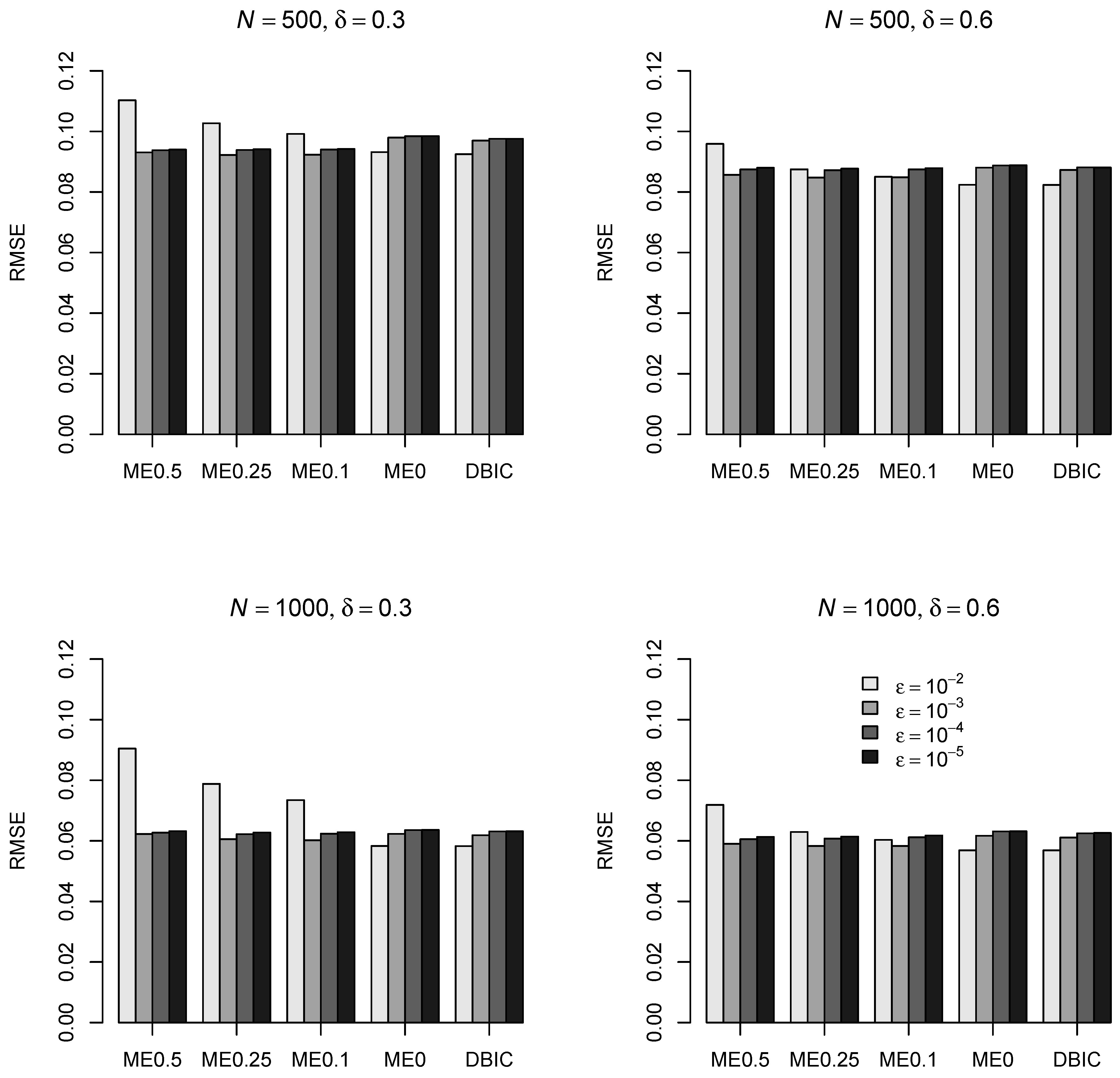
Figure 3 displays the RMSE of factor mean ${\alpha }_{2,1}$ in the second group for the different estimators for DIF effect sizes $\mathsf{\delta }=0.3$ and $\mathsf{\delta }=0.6$ and sample sizes $N=500$ and $N=1000$ as a function of the tuning parameter $\mathsf{\epsilon }$. It can be seen that $\mathsf{\epsilon }={10}^{-3}$ was optimal with respect to the RMSE for ME0.5, ME0.25, and ME0.1, while $\mathsf{\epsilon }={10}^{-2}$ resulted in the smallest RMSE for ME0 and DBIC. The findings were very similar for the factor mean ${\alpha }_{3,1}$ in the third group and the sample sizes $N=250$ and $N=2000$.

Table 1. Simulation Study 1: Bias and relative root mean square error (RMSE) of factor means and factor variances as a function of DIF effect size $\mathsf{\delta }$ and sample size N.

			Bias						Relative RMSE
Par	$\mathsf{\delta }$	$\mathbf{N}$	ML	ME0.5	ME0.25	ME0.1	ME0	DBIC	ML	ME0.5 ${}^{†}$	ME0.25	ME0.1	ME0	DBIC
${\alpha }_{2,1}$	0	250	$\phantom{-}$0.001	$\phantom{-}$0.002	$\phantom{-}$0.002	$\phantom{-}$0.002	$\phantom{-}$0.002	$\phantom{-}$0.002	97.5	100.0	101.3	102.0	101.2	101.1
		500	$\phantom{-}$0.000	$\phantom{-}$0.000	$\phantom{-}$0.000	$\phantom{-}$0.000	$\phantom{-}$0.000	$\phantom{-}$0.000	98.5	100.0	100.8	101.4	100.0	100.0
		1000	$\phantom{-}$0.001	$\phantom{-}$0.000	$\phantom{-}$0.000	$\phantom{-}$0.000	$\phantom{-}$0.000	$\phantom{-}$0.000	99.1	100.0	100.5	100.9	99.5	99.5
		2000	$\phantom{-}$0.001	$\phantom{-}$0.001	$\phantom{-}$0.001	$\phantom{-}$0.001	$\phantom{-}$0.001	$\phantom{-}$0.001	99.6	100.0	100.3	100.5	99.6	99.3
	0.3	250	−0.119	−0.061	−0.055	−0.054	−0.048	−0.048	114.9	100.0	101.2	102.2	104.3	104.3
		500	−0.119	−0.034	−0.026	−0.023	−0.015	−0.015	152.9	100.0	98.9	99.1	100.0	99.4
		1000	−0.120	−0.021	−0.014	−0.011	−0.005	−0.005	211.9	100.0	97.3	96.7	93.4	93.2
		2000	−0.120	−0.015	−0.009	−0.007	−0.004	−0.004	293.2	100.0	96.0	95.2	93.2	93.4
	0.6	250	−0.239	−0.034	−0.023	−0.019	−0.005	−0.005	215.0	100.0	99.0	98.9	97.1	97.1
		500	−0.238	−0.018	−0.011	−0.008	$\phantom{-}$0.000	$\phantom{-}$0.000	293.3	100.0	99.4	99.7	96.6	96.6
		1000	−0.239	−0.013	−0.007	−0.005	−0.001	−0.001	417.8	100.0	98.7	98.7	96.5	96.5
		2000	−0.238	−0.009	−0.004	−0.003	$\phantom{-}$0.000	$\phantom{-}$0.000	598.0	100.0	98.2	98.1	96.8	97.0
${\alpha }_{3,1}$	0	250	$\phantom{-}$0.005	$\phantom{-}$0.005	$\phantom{-}$0.005	$\phantom{-}$0.005	$\phantom{-}$0.005	$\phantom{-}$0.004	96.8	100.0	101.2	101.8	101.7	101.8
		500	$\phantom{-}$0.002	$\phantom{-}$0.002	$\phantom{-}$0.002	$\phantom{-}$0.002	$\phantom{-}$0.002	$\phantom{-}$0.002	97.8	100.0	101.1	101.8	100.3	100.4
		1000	$\phantom{-}$0.002	$\phantom{-}$0.002	$\phantom{-}$0.002	$\phantom{-}$0.002	$\phantom{-}$0.002	$\phantom{-}$0.002	98.9	100.0	100.7	101.1	99.4	99.5
		2000	$\phantom{-}$0.001	$\phantom{-}$0.001	$\phantom{-}$0.001	$\phantom{-}$0.001	$\phantom{-}$0.001	$\phantom{-}$0.001	99.4	100.0	100.3	100.6	99.6	99.3
	0.3	250	−0.110	−0.058	−0.053	−0.051	−0.045	−0.045	112.0	100.0	101.2	102.1	104.3	104.1
		500	−0.113	−0.033	−0.025	−0.022	−0.014	−0.014	147.0	100.0	99.2	99.5	100.0	99.6
		1000	−0.115	−0.021	−0.013	−0.010	−0.004	−0.004	203.3	100.0	97.3	96.9	93.7	93.5
		2000	−0.115	−0.015	−0.009	−0.007	−0.003	−0.003	280.3	100.0	96.1	95.3	93.3	93.5
	0.6	250	−0.218	−0.032	−0.021	−0.017	−0.003	−0.004	197.0	100.0	99.6	99.8	98.7	99.0
		500	−0.217	−0.017	−0.009	−0.007	$\phantom{-}$0.002	$\phantom{-}$0.001	268.5	100.0	99.9	100.3	97.6	97.6
		1000	−0.219	−0.012	−0.006	−0.004	$\phantom{-}$0.001	$\phantom{-}$0.000	376.6	100.0	99.2	99.4	97.2	97.2
		2000	−0.220	−0.009	−0.005	−0.003	$\phantom{-}$0.000	$\phantom{-}$0.000	539.6	100.0	98.3	98.2	96.9	97.1
${\varphi }_{2,11}$	0	250	$\phantom{-}$0.012	$\phantom{-}$0.015	$\phantom{-}$0.016	$\phantom{-}$0.016	$\phantom{-}$0.016	$\phantom{-}$0.016	97.2	100.0	101.0	101.7	102.6	102.6
		500	$\phantom{-}$0.007	$\phantom{-}$0.009	$\phantom{-}$0.009	$\phantom{-}$0.009	$\phantom{-}$0.009	$\phantom{-}$0.009	98.0	100.0	100.8	101.3	101.3	101.4
		1000	$\phantom{-}$0.007	$\phantom{-}$0.008	$\phantom{-}$0.008	$\phantom{-}$0.008	$\phantom{-}$0.007	$\phantom{-}$0.007	98.6	100.0	100.6	101.0	100.2	100.3
		2000	$\phantom{-}$0.003	$\phantom{-}$0.003	$\phantom{-}$0.003	$\phantom{-}$0.003	$\phantom{-}$0.003	$\phantom{-}$0.003	99.0	100.0	100.3	100.6	99.9	99.9
	0.3	250	$\phantom{-}$0.017	$\phantom{-}$0.020	$\phantom{-}$0.021	$\phantom{-}$0.021	$\phantom{-}$0.021	$\phantom{-}$0.021	96.9	100.0	100.9	101.4	102.7	102.8
		500	$\phantom{-}$0.007	$\phantom{-}$0.008	$\phantom{-}$0.008	$\phantom{-}$0.009	$\phantom{-}$0.008	$\phantom{-}$0.009	98.5	100.0	100.7	101.2	101.2	101.2
		1000	$\phantom{-}$0.002	$\phantom{-}$0.003	$\phantom{-}$0.003	$\phantom{-}$0.003	$\phantom{-}$0.002	$\phantom{-}$0.002	99.0	100.0	100.6	101.0	100.3	100.3
		2000	$\phantom{-}$0.002	$\phantom{-}$0.002	$\phantom{-}$0.002	$\phantom{-}$0.002	$\phantom{-}$0.001	$\phantom{-}$0.001	99.5	100.0	100.3	100.5	99.9	99.9
	0.6	250	$\phantom{-}$0.018	$\phantom{-}$0.020	$\phantom{-}$0.021	$\phantom{-}$0.022	$\phantom{-}$0.023	$\phantom{-}$0.023	97.9	100.0	100.8	101.3	102.5	102.5
		500	$\phantom{-}$0.010	$\phantom{-}$0.008	$\phantom{-}$0.008	$\phantom{-}$0.008	$\phantom{-}$0.008	$\phantom{-}$0.009	99.1	100.0	100.8	101.3	101.2	101.4
		1000	$\phantom{-}$0.007	$\phantom{-}$0.004	$\phantom{-}$0.004	$\phantom{-}$0.004	$\phantom{-}$0.004	$\phantom{-}$0.004	99.7	100.0	100.6	101.1	100.1	100.1
		2000	$\phantom{-}$0.004	$\phantom{-}$0.001	$\phantom{-}$0.001	$\phantom{-}$0.001	$\phantom{-}$0.001	$\phantom{-}$0.001	100.2	100.0	100.3	100.5	99.9	99.9
${\varphi }_{3,11}$	0	250	$\phantom{-}$0.011	$\phantom{-}$0.012	$\phantom{-}$0.013	$\phantom{-}$0.013	$\phantom{-}$0.013	$\phantom{-}$0.013	96.7	100.0	101.4	102.2	103.3	103.2
		500	$\phantom{-}$0.005	$\phantom{-}$0.006	$\phantom{-}$0.006	$\phantom{-}$0.006	$\phantom{-}$0.006	$\phantom{-}$0.006	97.9	100.0	100.9	101.5	101.3	101.4
		1000	$\phantom{-}$0.005	$\phantom{-}$0.005	$\phantom{-}$0.005	$\phantom{-}$0.005	$\phantom{-}$0.005	$\phantom{-}$0.005	98.6	100.0	100.7	101.2	100.3	100.4
		2000	$\phantom{-}$0.002	$\phantom{-}$0.002	$\phantom{-}$0.002	$\phantom{-}$0.002	$\phantom{-}$0.002	$\phantom{-}$0.002	98.8	100.0	100.4	100.7	99.9	99.9
	0.3	250	$\phantom{-}$0.015	$\phantom{-}$0.015	$\phantom{-}$0.015	$\phantom{-}$0.015	$\phantom{-}$0.016	$\phantom{-}$0.016	97.3	100.0	101.0	101.7	103.2	103.1
		500	$\phantom{-}$0.005	$\phantom{-}$0.006	$\phantom{-}$0.006	$\phantom{-}$0.006	$\phantom{-}$0.006	$\phantom{-}$0.006	98.2	100.0	101.0	101.6	101.4	101.5
		1000	$\phantom{-}$0.002	$\phantom{-}$0.002	$\phantom{-}$0.002	$\phantom{-}$0.002	$\phantom{-}$0.002	$\phantom{-}$0.002	98.7	100.0	100.7	101.2	100.3	100.3
		2000	$\phantom{-}$0.002	$\phantom{-}$0.002	$\phantom{-}$0.002	$\phantom{-}$0.002	$\phantom{-}$0.002	$\phantom{-}$0.002	99.6	100.0	100.3	100.5	99.9	99.9
	0.6	250	$\phantom{-}$0.015	$\phantom{-}$0.015	$\phantom{-}$0.016	$\phantom{-}$0.016	$\phantom{-}$0.016	$\phantom{-}$0.016	98.5	100.0	101.3	102.0	103.4	103.5
		500	$\phantom{-}$0.008	$\phantom{-}$0.007	$\phantom{-}$0.007	$\phantom{-}$0.007	$\phantom{-}$0.007	$\phantom{-}$0.007	98.8	100.0	101.1	101.6	101.4	101.5
		1000	$\phantom{-}$0.005	$\phantom{-}$0.004	$\phantom{-}$0.004	$\phantom{-}$0.004	$\phantom{-}$0.004	$\phantom{-}$0.004	99.4	100.0	100.8	101.3	100.2	100.2
		2000	$\phantom{-}$0.002	$\phantom{-}$0.001	$\phantom{-}$0.001	$\phantom{-}$0.001	$\phantom{-}$0.001	$\phantom{-}$0.001	99.9	100.0	100.4	100.6	99.9	99.9

Note. Par = parameter; α_g,1 = factor mean in group g = 2, 3; ϕ_g,11 = factor variance in group g = 2, 3; ML = maximum likelihood estimation; MEp = robust moment estimation with p = 0.5 (with ε = 0.001), p = 0.25 (with ε = 0.001), p = 0.1 (with ε = 0.001), or p = 0 (with ε = 0.01); DBIC = direct BIC minimization (with ε = 0.01). Absolute biases larger than 0.015 are shown with a gray background. ^† ME0.5 is the reference method in the computation of the relative RMSE. Relative RMSE values smaller than 98.0 are printed in bold font. Relative RMSE values larger than 102.0 are show with a gray background.

displays the bias and relative RMSE of factor means and factor variances as a function of the DIF effect size and the sample size for the different estimation methods. We chose the tuning parameter $\mathsf{\epsilon }={10}^{-3}$ for the estimators ME0.5, ME0.25, and ME0.1, and $\mathsf{\epsilon }={10}^{-2}$ for the estimators ME0 and DBIC because they resulted in the smallest RMSE of factor means according to the findings of Figure 3.

Overall, all estimators except for ML were approximately unbiased for factor variances in all conditions and for factor means in the absence of DIF effects (i.e., $\mathsf{\delta }=0$ and measurement invariance holds) except for the sample size $N=250$. Slightly biased estimates were obtained for ME with a larger p, such as $p=0.5$ in ME0.5. However, the bias decreased with increasing sample size. The ME0 and DBIC were unbiased across all conditions, followed by the estimators ME0.1, ME0.25, and ME0.5, with increasing absolute bias. There was substantial bias for estimated factor means for ML estimation, while the estimates of factor variances were approximately unbiased for ML.

To compare the estimation accuracy in terms of the relative RMSE, we chose ME0.5 (with $\mathsf{\epsilon }={10}^{-3}$) as the reference model. Hence, the relative RMSE was 100 for this method in Table 1. It turned out that ME0 and DBIC were superior to the other estimators with non-negligible efficiency gains. For example, for the factor mean ${\alpha }_{2,1}$ in the second group, $\mathsf{\delta }=0.3$, and $N=1000$, the efficiency gain in terms of the RMSE was 6.4% (=100 − 93.6) for ME0 and 6.5% for DBIC. Across all conditions, no noteworthy differences between ME0 and DBIC estimators were found.

ML estimates were slightly more efficient than ME estimates in the absence of DIF. However, the efficiency gains of ML decrease with increasing sample size.

To conclude, it seems promising to replace the $L_p$ loss function using the power $p=0.5$ (i.e., ME0.5) with the $L_0$ loss function implemented in ME0 or regularized estimation in DBIC for large sample sizes $N=1000$ or $N=2000$. Similar performance of the different estimators was found for $N=500$, while the power $p=0.5$ was the frontrunner for $N=250$.

7. Simulation Study 2: Coverage

The second Simulation Study 2 investigated the assessment of coverage rates of the model-robust moment estimators and the DBIC method.

7.1. Method

The same DGM as in Simulation Study 1 was employed to simulate data (see Section 6.1). We evaluated the standard error computation described in Section 4 for the five estimators using the tuning parameter $\mathsf{\epsilon }$ that resulted in the smallest RMSE of factor means. In detail, we used $\mathsf{\epsilon }={10}^{-3}$ for the estimators ME0.5, ME0.25, and ME0.1; and we used $\mathsf{\epsilon }={10}^{-2}$ for the estimators ME0 and DBIC (see Figure 3). Moreover, we included ML estimation for reasons of comparison.

The same analysis models as in Simulation Study 1 were specified. Confidence intervals at the confidence level of 95% were computed using a normal distribution approximation (i.e., the estimated confidence interval was $\widehat{\theta }\pm 1.96\times \mathrm{SE}\left(\widehat{\theta }\right)$). The coverage rate at the confidence level of 95% was computed as the percentage of the events that a computed confidence interval covers the true parameter value.

As in Simulation Study 1, 5000 replications were conducted in each of the 12 simulation conditions (i.e., 3 (DIF effect size $\mathsf{\delta }$) × 4 (sample size N) = 12 conditions). The SEMs with standard error estimates of model parameters were again estimated with the sirt::mgsem() function in the R [47] package sirt (Version 4.0-19; ref. [48]). Material for replication can be found at https://osf.io/ng6s3 (accessed on 25 September 2023).

7.2. Results

Table 2. Simulation Study 2: Coverage rates (in percentages) of factor means and factor variances as a function of DIF effect size $\mathsf{\delta }$ and sample size N.

Par	$\mathsf{\delta }$	N	ML	ME0.5	ME0.25	ME0.1	ME0	DBIC
${\alpha }_{2,1}$	0	250	94.7	96.6	97.1	97.2	96.5	96.6
		500	95.2	96.3	96.6	96.8	96.1	96.2
		1000	94.9	95.5	95.7	96.0	95.3	95.3
		2000	95.0	95.4	95.6	95.8	95.2	95.3
	0.3	250	80.3	95.4	96.3	96.8	96.1	95.6
		500	66.0	95.6	96.4	96.7	96.2	95.9
		1000	39.8	95.0	96.0	96.3	95.7	95.7
		2000	13.2	93.0	94.3	94.6	94.1	94.2
	0.6	250	42.8	96.3	96.9	97.1	96.3	92.1
		500	14.5	95.2	95.8	96.0	95.2	95.2
		1000	1.0	95.6	96.3	96.4	95.7	95.7
		2000	0.0	95.2	95.6	95.9	95.6	95.5
${\alpha }_{3,1}$	0	250	95.2	97.3	97.6	97.8	97.2	97.2
		500	95.0	96.3	97.0	97.3	96.0	96.1
		1000	95.3	96.0	96.3	96.6	95.6	95.6
		2000	94.9	95.3	95.5	95.7	95.1	95.2
	0.3	250	81.5	95.7	96.8	97.3	96.7	96.0
		500	68.6	95.0	96.5	96.8	95.8	95.7
		1000	44.9	95.4	96.3	96.7	95.7	95.8
		2000	16.3	93.5	94.5	94.8	94.3	94.1
	0.6	250	48.8	96.4	97.2	97.4	96.9	92.4
		500	21.3	95.8	96.7	96.8	96.0	95.9
		1000	2.5	95.3	96.3	96.7	95.6	95.6
		2000	0.1	95.0	95.5	95.8	95.3	95.3
${\varphi }_{2,11}$	0	250	94.8	96.8	97.2	97.5	97.2	97.2
		500	94.9	96.7	97.2	97.3	96.8	96.8
		1000	94.6	95.5	96.0	96.2	95.3	95.4
		2000	94.9	95.4	95.7	95.9	95.3	95.2
	0.3	250	94.6	96.7	97.2	97.4	97.2	97.2
		500	95.5	96.9	97.4	97.6	97.0	97.0
		1000	95.1	96.1	96.4	96.6	96.0	96.0
		2000	94.8	95.5	95.8	96.0	95.2	95.2
	0.6	250	94.9	96.8	97.3	97.4	97.2	97.1
		500	94.7	96.0	96.5	96.8	96.2	96.1
		1000	95.2	96.0	96.3	96.6	96.0	96.1
		2000	94.9	95.3	95.6	95.8	95.1	95.2
${\varphi }_{3,11}$	0	250	94.6	97.0	97.5	97.8	97.4	97.3
		500	95.1	96.9	97.2	97.4	97.0	97.0
		1000	94.6	95.8	96.2	96.5	95.8	95.9
		2000	95.0	95.5	95.9	96.2	95.4	95.4
	0.3	250	94.4	96.8	97.3	97.5	97.3	97.2
		500	95.1	96.9	97.3	97.5	96.8	96.8
		1000	94.7	96.0	96.3	96.6	96.0	96.0
		2000	95.2	95.8	96.2	96.3	95.6	95.7
	0.6	250	94.8	97.1	97.6	97.8	97.4	97.3
		500	95.2	97.1	97.5	97.7	97.0	96.8
		1000	95.2	95.9	96.5	96.9	96.0	96.0
		2000	94.6	95.1	95.4	95.7	94.9	94.9

Note. Par = parameter; α_g,1 = factor mean in group g = 2, 3; ϕ_g,11 = factor variance in group g = 2, 3; ML = maximum likelihood estimation; MEp = robust moment estimation with p = 0.5 (with ε = 0.001), p = 0.25 (with ε = 0.001), p = 0.1 (with ε = 0.001), or p = 0 (with ε = 0.01); DBIC = direct BIC minimization (with ε = 0.01); Coverage rates smaller than 91.0 or larger than 98.0 are shown with a gray background.

shows the coverage rates of factor means and factor variances for the five different estimators as a function of DIF effects size and sample size. Overall, the coverage rates were acceptable because they were neither smaller than 91.0 nor larger than 98.0 (see [49]). Across all conditions and estimators (when excluding ML estimation), the coverage rates in Table 2 ranged between 92.1 and 97.8, with a mean of $M=96.16$ and a standard deviation of $SD=0.93$. The coverage rates of ME0.5 ($M=95.87$, $SD=0.87$), ME0 ($M=96.03$, $SD=0.82$), DBIC ($M=95.81$, $SD=1.09$) performed slightly better than ME0.25 ($M=96.42$, $SD=0.78$) and ME0.1 ($M=96.67$, $SD=0.76$). The coverage rates for ML estimation ($M=74.57$, $SD=33.43$) were not acceptable for factor means which had biased estimates in the presence of DIF effects.

8. Discussion

In this article, we compared model-robust moment estimation with a recently proposed variant of regularized ML estimation by O’Neill and Burke [15] that directly maximizes the BIC (i.e., the DBIC estimator). In the DBIC estimation, these authors suggested a differentiable approximation of the $L_0$ loss function, which was also used in model-robust moment estimation. Interestingly, the $L_0$ loss function outperformed $L_p$ loss functions for $p>0$ regarding bias and RMSE. Furthermore, model-robust moment estimation with the $L_0$ loss function performed very similarly to the DBIC estimator. Moreover, the estimation of standard errors was successfully implemented for all estimators because coverage rates were acceptable for all parameters in all simulation conditions.

In line with previous studies, we anticipate that sample sizes must be sufficiently large in order to achieve the model-robustness properties of the $L_p$ and $L_0$ loss functions. If the sample size is too small (e.g., $N=100$ subjects in a multiple-group SEM analysis), the sampling error in moments that are used as sufficient statistics in the SEM can exceed model errors (i.e., unmodeled group-specific item intercepts). In this case, model-robust methods are not expected to perform well. In fact, Simulation Study 1 revealed that $p=0.5$ is preferable to other $L_p$ loss functions with $p<0.5$ or the $L_0$ loss function for $N=250$, while the situation changes with larger sample sizes such as $N=1000$.

Simulation Study 1 indicated that the tuning parameter $\mathsf{\epsilon }=0.001$ in the differentiable approximation of the nondifferentiable $L_p$ loss function should be used for the $L_p$ loss function for $p=0.5$, $p=0.25$, or $p=0.1$. In contrast, $\mathsf{\epsilon }=0.01$ was found optimal for the $L_0$ loss function and the direct BIC minimization estimation approach in regularized estimation. We expect that these findings will transfer to other models that involve standardized variables. In our experience from regularized estimation and the invariance alignment approach [21], using a value of $\mathsf{\epsilon }$ (such as $\mathsf{\epsilon }={10}^{-5}$ and smaller values) tuning parameter that is too small is prohibitive because it more likely results in convergence issues in the local optima of the fit function.

In our simulation studies, we only considered model errors in item intercepts. Future simulation studies could also investigate model errors in the covariance structure (i.e., unmodeled residual correlations). Of course, model errors in the mean and the covariance structure can also be simultaneously examined.

A requirement to achieve model robustness of SEM estimators is that model errors in the mean or covariance structure are sparsely distributed. That is, only a few entries are allowed to differ from zero, while the majority of model errors must be (approximately) zero. If factor loadings were not invariant across groups, more densely distributed model errors would result. As a consequence, model-robust moment estimation will likely not work, and regularized maximum likelihood estimation might be preferred. However, the DBIC minimization method for regularized maximum likelihood estimation can also be utilized in this case if the number of group-specific factor loadings is counted in the BIC penalty term.

In this article, we only applied the $L_0$ and $L_p$ loss functions to continuous items. However, the principle directly transfers to SEMs of ordinal data that are based on fitting thresholds and polychoric correlations [50] instead of means and covariances for continuous data, respectively. Moreover, the model-robust estimators could also be applied to two-step estimation methods of multilevel structural equation models [51,52].

To sum up, model-robust SEM estimators based on the $L_p$ (for $p<1$) and $L_0$ loss functions are attractive to researchers who do not want model estimates being influenced by the presence of a few model deviations (i.e., model errors). In contrast, usually employed (non-robust) SEM estimators such as maximum likelihood estimation are impacted by model errors. In this sense, misfitting models do not necessarily result in biased estimates when using model-robust estimation.