Expanding NAEP and TIMSS Analysis to Include Additional Variables or a New Scoring Model Using the R Package Dire

Abstract

The R packages Dire and EdSurvey allow analysts to make a conditioning model with new variables and then draw new plausible values. This is important because results for a variable not in the conditioning model are biased. For regression-type analyses, users can also use direct estimation to estimate parameters without generating new plausible values. Dire is distinct from other available software in R in that it requires fixed item parameters and simplifies calculation of high-dimensional integrals necessary to calculate composite or subscales. When used with EdSurvey, it is very easy to use published item parameters to estimate a new conditioning model. We show the theory behind the methods in Dire and a coding example where we perform an analysis that includes simple process data variables. Because the process data is not used in the conditioning model, the estimator is biased if a new conditioning model is not added with Dire.

1. Introduction

Large-scale assessments (LSA), such as the U.S. National Assessment of Educational Progress (NAEP) and the Trends in International Mathematics and Science Study (TIMSS), use plausible values to accurately estimate population estimates of respondent performance [1]. Plausible values are used in LSA because traditional item response theory models result in biased estimates of population parameters (Note that an LSA with a high-reliability assessment would not need to use plausible values). Plausible values are routinely generated by the statistical agency responsible for the data collection, and can be used to generate unbiased population estimates (Conditional on the validity of the survey sampling strategy and psychometric instrument. These are not minor issues, but they are not the focus of this paper). These plausible values come from a conditioning model that includes information from all background variables, generally through a dimension reduction (i.e., principal component analysis) on the full set of covariates. However, when the analyst brings in data not available to the statistical agency, or they incorporate data on the file but not yet synthesized on the file—such as many results derived from process data—they will need to generate new plausible values with a new conditioning model to obtain unbiased regression parameters. (PISA includes some process data variables [2]. Though any such attempt only scratches the surface of process data variables [3].) In addition, if the question of interest can be stated as a regression, direct estimation, where the coefficients from the conditioning model itself are used, is an unbiased estimator of the regression coefficients [4].

This paper describes the methods of the Dire package for direct estimation and generation of new plausible values (Dire 2.1.1 CRAN: https://cran.r-project.org/web/packages/Dire/index.html, GitHub: https://github.com/American-Institutes-for-Research/Dire, Vignette: https://cran.r-project.org/web/packages/Dire/vignettes/MML.pdf (accessed on 16 August 2023)). The existing TAM software performs all of the necessary steps to go from item responses to estimate item parameters and produce new plausible values [5]. Dire, especially when paired with EdSurvey [6], instead focuses on estimating new latent regression models and plausible values for LSA where the user wants to use the existing item parameters published by the statistical agency sharing the results. In addition, Dire is intended to be able to estimate high-dimensional models used in NAEP where the mathematics scale is a composite of five correlated subscales, as well as TIMSS where four- (grade 4) or five- (grade 8) constructs are estimated in a multi-dimensional model to estimate subscales [7].

We show the model used by Dire to estimate a conditioning model. We then show the estimation strategy used by Dire to estimate high-dimensional models without suffering from exponential-time costs, and how plausible values are generated. We provide a simple example of using Dire to estimate a new conditioning model with EdSurvey; for completeness we also show how to estimate a toy example (that is not an existing LSA) in Dire without using EdSurvey.

2. Background

Typically, student ability is estimated by a factor score (e.g., EAP, WLE, or MLE) of a corresponding IRT model. Those student abilities can then be used in subsequent analysis. With a high-reliability test, this is a valid method of analysis because the measurement error represents a small portion of the total test variance. As such, many existing methods for IRT available in R [8] focus on estimation of a $\theta$ for each student, which can then be used in subsequent analysis.

LSA are designed to estimate population characteristics directly and do not provide estimates of individual scores. They instead provide random draws from distributions for individual proficiencies in the form of plausible values.

It is possible to estimate plausible values using proprietary software such as Mplus [9]. For users who are interested in open source software, R [8] has become popular as a way to share software and methods.

In the R psychometrics view [10], a few packages have capabilities for drawing plausible values (the focus of the Dire package): TAM [5], mirt [11], and Dire. Additionally, the NEPSscaling package may be used to draw plausible values focusing on data from the German National Educational Panel Study (NEPS) [12]. The models shown in this paper may be fit with TAM, mirt, or Dire. In contrast to mirt and TAM, Dire uses a different method of calculating the multi-dimensional integral. Where TAM and mirt calculate a multi-dimensional integral by calculating all of the dimensions at once, Dire does so one- or two-dimensions at a time. When Dire estimates the conditioning model, it uses the existing item parameters. The EdSurvey package will download and format them for NAEP and TIMSS data for the user so that the process is seamless.

The methods in Dire, similar to other plausible value approaches, mirror those used in the statistical package AM [13] and result in unbiased estimates of parameters included in the conditioning model [1,4].

The Dire package is integrated into the EdSurvey package, which allows users to download, read in, manipulate, and analyze U.S. NCES, IEA, and OECD LSA data. For a detailed overview of the functionality of the EdSurvey package, see [6]. This paper synthesizes portions of the methodology covered in the Dire vignette with worked examples to provide an overview of the methods and application of Dire in analyzing LSA data.

3. Methodology in Dire

Generating plausible values requires first estimating a marginal maximum likelihood (MML) model, (Note that we refer to the model as using a log-likelihood throughout this paper, but the model is weighted by survey sample weights for each student and so it is correctly a pseudo log-likelihood. One important implication of this is that likelihood ratio tests are not valid, so the absolute values of the modeled likelihoods are not relevant) and then estimating a posterior distribution for each test taker, conditional on the model and the test taker’s responses [14]. The regression coefficients in the marginal maximum likelihood model can be used directly in a process known as direct estimation [4]. The methodology described in the following sections allows for efficient and accurate recovery of model parameters [4].

3.1. Marginal Maximum Likelihood

3.1.1. Likelihood

MML estimation extends the methodology of standard maximum likelihood (ML) estimation to situations where variables of interest are latent (not directly observable), such as student math ability. The principal difference is that the latent variable is not assumed to be known and is thus integrated out over a distribution of possible values—that this step is analogous to multiple imputation is one of the key insights of [1].

In MML estimation, an individual student’s likelihood has two components: (1) the probability of observing the student’s item responses, given their latent ability, and (2) the probability that a student with a given set of covariate levels would have this student ability, conditional on the regression coefficients and the residual variance. The product of these two terms is then integrated out over all possible student ability levels—this is the marginalization in MML.

The first component, the probability of observing the student’s item responses, is captured by an item response theory (IRT) model dependent upon the item parameters, and the student’s score on the item. The latter component is the latent regression model and is modeled as a normal distribution with ${\mathit{X}}_i\mathsf{\beta }$, where ${\mathit{X}}_i$ is student i’s ($i=1,\dots ,N$) covariates in an $m\times 1$ row vector, and $\mathsf{\beta }$ are the m regression parameters associated with that vector. In the uni-dimensional case, we define the latent regression model as

$${\theta }_i={\mathit{X}}_i\mathsf{\beta }+{ϵ}_i,{ϵ}_i\sim N(0,\sigma ),$$

(1)

where $N(0,\sigma )$ is a normal distribution with mean zero and standard deviation $\sigma$. The assumption follows that the conditional distribution of ${\theta }_i$ is $f\left({\theta }_i\right|{\mathit{X}}_i\mathsf{\beta },\sigma )$, where f represents the normal density function. The full likelihood function for a single construct for student i is then represented as

$$\begin{array}{c}\hfill \mathcal{L}(\mathsf{\beta },\sigma ;{\mathit{R}}_i,{\mathit{X}}_i,\mathit{P})=\int {\left[f\left({\theta }_i\right|{\mathit{X}}_i\mathsf{\beta },\sigma )·\prod _{h=1}^H\mathrm{Pr}\left(R_{ih}\right|{\theta }_i,{\mathit{P}}_h)\right]}^{w_i}d{\theta }_i,\end{array}$$

(2)

where $R_{ih}$ represents student i’s response to item h, ${\theta }_i$ is student i’s latent ability, $w_i$ is the sampling weight for student i, ${\mathit{P}}_h$ is the vector of item parameters for item h, and the student sees H items [An added complication is that students do not take the same assessment. TIMSS takes the full assessment pool and generates 14 different student achievement booklets through matrix sampling, such that each item will appear in two booklets. Students complete only one of these booklets and hence see only a fraction of the total items [15]; NAEP similarly uses rotated forms [16]. However, this issue is not discussed further because it represents only minor technical problems for MML that are ignored because it primarily adds notational complexity—for example, the items become student-specific, which would need to be indicated in the product over h]. Looking at the left hand side of the equation, ${\mathit{R}}_i$ is the vector of student i’s responses across the H items, and $\mathit{P}$ is a matrix whose rows are the vectors ${\mathit{P}}_h$, $h=1,\dots ,H$.

Here, ${\theta }_i$ is a random variable, while $R_{ih}$, ${\mathit{X}}_i$, and ${\mathit{P}}_h$ are fixed [In the context of LSA, the IRT parameters are generally estimated first and then treated as fixed when estimating the latent regression model [17,18]. These item parameter estimates are included on the data file, so Dire treats them as fixed]. The parameters to estimate are $\mathsf{\beta }$ and $\sigma$.

In the composite scoring framework, where overall ability is measured as a weighted sum of multiple potentially correlated subdimensions, things are considerably more complicated [Given the focus on LSA, similar to NAEP and TIMSS, Dire fits a between-item multidimensional model]. Now ${\mathsf{\theta }}_i$ is a vector, with an element for each construct, and dependence between the constructs is allowed by modeling the residual as a multivariate normal with residual $\Sigma$. We assume here that each item is associated with only one construct. The target integral to evaluate is then:

$$\begin{array}{c}\hfill \mathcal{L}({\mathsf{\beta }}_1,\dots ,{\mathsf{\beta }}_J,\Sigma ;{\mathit{R}}_i,{\mathit{X}}_i,\mathit{P})=\int \dots \int \frac{1}{{\left(2\pi \right)}^{\frac{J}{2}}\sqrt{\det (\Sigma )}}exp(-\frac{1}{2}{\mathsf{ϵ}}_i^T\Sigma {\mathsf{ϵ}}_i)\\ \hfill \prod _{j=1}^J\prod _{h=1}^{H_j}\mathrm{Pr}\left(R_{ijh}\right|{\theta }_{ij},{\mathit{P}}_{hj})d{\theta }_{i1}\dots d{\theta }_{iJ},\end{array}$$

(3)

where J is the number of constructs, and ${\mathsf{ϵ}}_i$ are the residuals ${\mathsf{\theta }}_i-{\mathit{X}}_i\mathsf{\beta }$ for student i. The terms here are analogous to those in Equation (2) but are now also indexed by the construct, i.e., $R_{ijh}$ is student i’s response to item h within construct j, ${\theta }_{ij}$ is student i’s latent ability in construct j, and ${\mathit{P}}_{hj}$ is the vector of item parameters for item h ($h=1,\dots ,H_j$) in construct j. For compactness, we have dropped the $w_i$ term here and in the next section, but the weighting is still implied. The integral in Equation (2) (and consequently in Equation (3), which generalizes Equation (2)) is intractable and thus requires numeric approximation.

3.1.2. Integral Approximation

Several methods have been proposed in the literature for high-dimensional integral approximation, including stochastic expectation maximization (EM), Metropolis–Hastings Robbins–Monro (MH-RM), and both fixed and adaptive quadrature [19]. Stochastic methods are considered more computationally efficient than numeric quadrature when the number of latent dimensions (i.e., number of constructs) exceeds three, as the requisite number of evaluations only increases linearly [20]. Adaptive quadrature tries to overcome this limitation by decreasing the number of points needed for accurate approximation, but is still subject to computational complexity that grows exponentially with the number of dimensions [21,22]. For a recent review of related methods, see [19].

With a large number of test items, the dispersion of the likelihood given the response patterns is small, and fixed point quadrature would inadequately approximate the likelihood [21,22]. However, in the context of LSA, relatively few items are administered to each student in a given subject. This results in a more dispersed likelihood that fixed point quadrature is suited to approximate. Additionally, in the uni-dimensional case, fixed quadrature has been shown to be more efficient than, e.g., MH-RM, with comparable accuracy [22]. Dire, following the methodology of [4], transforms the problem of approximating a multi-dimensional integral into one of estimating a uni-dimensional integral per subscale. To do this, we make the observation that the multi-dimensional case is analogous to a seemingly unrelated regression (SUR) model with identical regressors and normally distributed errors that are correlated across equations. It is shown in [23] that for this special case of a SUR model, estimates are no more efficient when regressors are estimated simultaneously vs. separately. We begin by writing the joint density as a product of a marginal and a conditional, as in Equation (4).

$$\begin{array}{cc}\mathcal{L}({\mathsf{\beta }}_1,\dots ,{\mathsf{\beta }}_J,\Sigma ;{\mathit{R}}_i,{\mathit{X}}_i,\mathit{P})=\hfill & \int f_1\left({ϵ}_{i1}\right)\left[\prod _{h=1}^{H_1}\mathrm{Pr}\left(R_{ih1}\right|{\theta }_{i1},{\mathit{P}}_{h1})\right]d{\theta }_{i1}·\hfill \\ \hspace{1em}& \hfill \int \dots \int f_{-1}\left({ϵ}_{i,-1}\right|{ϵ}_{i1})\prod _{j=2}^J\prod _{h=1}^{H_j}\mathrm{Pr}\left(R_{ijh}\right|{\theta }_{ij},{\mathit{P}}_{hj})d{\theta }_{i2}\dots d{\theta }_{iJ}.\end{array}$$

(4)

By partitioning the likelihood this way, we obtain an additively separable likelihood once logs are taken, allowing for maximization of each part of the likelihood independently.

In the context of SUR, one possible approach to estimation is the two-step procedure of iterated feasible generalized least squares (FGLS) [23]. In the first step, weighted least squares (WLS) is used to estimate regression coefficients. Residuals from these estimates are then used to estimate the covariance matrix. In the second step, the estimated covariance matrix is used to update the estimated coefficient matrix. While the first step is able to be decomposed for each latent variable, the second step cannot be when the latent variables are correlated [24]. As an alternative, we can estimate the parameters through direct maximization. To do so, we must approximate the uni-dimensional integral for each of j subscales. In this new context of a uni-dimensional integral (with theoretically high dispersion), fixed point quadrature is expected to perform well. Dire creates a fixed grid of integration points that the integral is then evaluated over. Because latent ability is assumed to follow a standard normal distribution when calibrating item difficulty, the default range for this grid is chosen to be $[-4,4]$. Within this range, 30 equidistant quadrature points are chosen by default. The user may specify an alternative range and number of quadrature points.

This quadrature representation is shown in Equation (5). Here, the integration nodes $t_q$ stand in for student latent ability, and $\delta$ is the distance between any two subsequent nodes. The term c is a constant that depends on the other dimensions (or constructs) that are now not a function of ${\mathsf{\beta }}_1$ nor the residual variance ${\sigma }_1^2={\Sigma }_{1,1}$ term.

$$\begin{array}{cc}\hfill \mathcal{L}({\mathsf{\beta }}_1,\dots ,{\mathsf{\beta }}_J,\Sigma ;{\mathit{R}}_i,{\mathit{X}}_i,\mathit{P})\approx & \left\{\sum _{q=1}^Q\delta f_1(t_q-{\mathit{X}}_i{\mathsf{\beta }}_1)\left[\prod _{h=1}^{H_1}\mathrm{Pr}\left(R_{i1h}\right|t_q,{\mathit{P}}_{h1})\right]\right\}·c.\hfill \end{array}$$

(5)

Instead of needing to optimize a multi-dimensional integral over all subscales simultaneously, the process is simplified considerably to:

• Estimate ${\mathsf{\beta }}_j$ and ${\sigma }_j$ for each subscale j by optimizing a univariate density (5) and
• Hold the ${\mathsf{\beta }}_j$ and ${\sigma }_j^2$ (the diagonal terms in $\Sigma$) estimates fixed and estimate the correlations for each of the $\left(\genfrac{}{}{0pt}{}{J}{2}\right)$ pairs of subscales (the non-diagonal elements of $\Sigma$).

The second step takes advantage of the fact that a multivariate normal is conditionally a multivariate normal distribution, after conditioning on a subset of the variables. The likelihood of the covariance between two subscales is defined as:

$$\begin{array}{cc}\hfill \mathcal{L}\left({\sigma }_{1,2}\right)=& \int \int f_{1,2}\left({ϵ}_{i(1,2)}\right)\left[\prod _{j=1}^2\prod _{h=1}^{H_j}\mathrm{Pr}\left(R_{ijh}\right|{\theta }_{ij},{\mathit{P}}_{hj})\right]d{\theta }_{i1}d{\theta }_{i2}·\hfill \\ \hspace{1em}& \int \dots \int f_{(3,\dots ,J)}\left({ϵ}_{i(3,\dots ,J)}\right|{ϵ}_{i(1,2)})\prod _{j=3}^J\prod _{h=1}^{H_j}\mathrm{Pr}\left(R_{ijh}\right|{\theta }_{ij},{\mathit{P}}_{hj})d{\theta }_{i3}\dots d{\theta }_{iJ}\hfill \end{array}$$

(6)

$$\begin{array}{c}\hspace{1em}\hspace{1em}\hspace{0.17em}=\int \int f_{1,2}\left({ϵ}_{i(1,2)}\right)\left[\prod _{j=1}^2\prod _{h=1}^{H_j}\mathrm{Pr}\left(R_{ijh}\right|{\theta }_{ij},{\mathit{P}}_{hj})\right]d{\theta }_{i1}d{\theta }_{i2}·c^{\prime },\hfill \end{array}$$

(7)

where the left-hand side has been simplified to indicate the only parameter being estimated is ${\sigma }_{1,2}$, the covariance between subscales one and two. Here, $f_{1,2}\left({ϵ}_{i(1,2)}\right)$ is the bivariate normal distribution, evaluated at a mean of ${ϵ}_{i(1,2)}$, with covariance matrix having diagonal elements ${\sigma }_1,{\sigma }_2$ and off-diagonal elements both ${\sigma }_{1,2}$. The second integral is the multivariate normal distribution of all other variables, conditional on the first two values. Because this second term is a constant, it can be replaced with the term $c^{\prime }$ and ignored when maximizing the integral.

3.2. Parameter Estimation

3.2.1. Estimating $\beta$ and $\sigma$

To estimate the $\mathsf{\beta }$ and $\sigma$ terms, we plug in the normal distribution for f and use the univariate objective function in Equation (5) which can be maximized accordingly by dropping the trailing c term (because it is irrelevant for maximization). We once again make the survey sample weighting explicit and define the log-likelihood:

$$\begin{array}{cc}\hfill \mathsf{\ell }(\mathsf{\beta },\sigma ;\mathit{w},\mathit{R},\mathit{X},\mathit{P})& \approx \sum _{i=1}^N{\mathit{w}}_i\log \left[\delta \sum _{q=1}^Q\frac{1}{\sigma \sqrt{2\pi }}exp\frac{-{(t_q-{\mathit{X}}_i\mathsf{\beta })}^2}{2{\sigma }^2}\prod _{h=1}^H\mathrm{Pr}\left({\mathit{R}}_{ih}\right|t_q,{\mathit{P}}_h)\right],\hfill \end{array}$$

(8)

where as before the integration nodes $t_q$ stand in for the latent ability, previously labeled ${\theta }_i$, $\delta$ is the distance between any subsequent node pair, and $w_i$ is the sampling weight for student i. As we are now summing across all students, we let $\mathit{w}$ denote the vector of student sample weights, while $\mathit{R}$ is an $N\times H$ matrix of student item responses, and $\mathit{X}$ is the $N\times m$ design matrix. The first component of this likelihood is the univariate normal of the residuals, ${ϵ}_i$. The second component is the probability of student i’s responses, given the item parameters and the node. Item scoring may be 3-PL, graded response, or partial credit (see the Dire documentation for how to specify the parameters).

The full likelihood for a given student is comprised of the density of their latent ability and the product of their response probabilities across all items, each respective to the appropriate IRT model. To make this computation more efficient, Dire calculates the item response likelihoods outside of the optimized function, since these do not depend on $\mathsf{\beta }$ and $\sigma$. The optimization then only takes place over the univariate normal portion of the likelihood. Dire takes a robust approach to optimization that begins with using the memory-efficient L-BFGS-B algorithm to identify a maximum. Because the L-BFGS-B implementation programmed in R does not have a convergence criterion based on the gradient, Dire further refines these estimates with a series of Newton steps, using the gradient as a convergence criterion—since a maximum has zero gradient, by definition. Because the integration nodes and item parameters are fixed during optimization, the term $\mathrm{Pr}\left(R_{ih}\right|t_q,{\mathit{P}}_h)$ will not change over the surface of $\mathsf{\beta }$ or $\sigma$, so it is only necessary to evaluate it once per student over the grid.

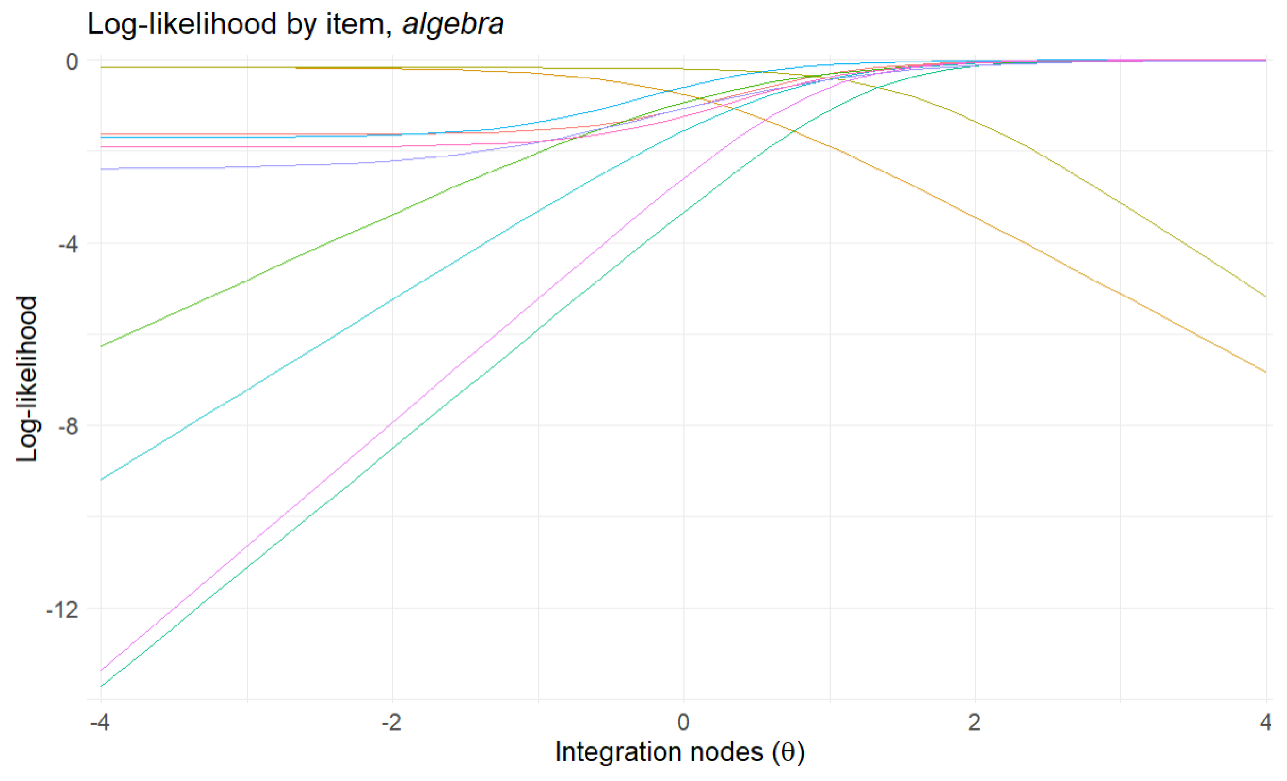
To demonstrate this, we consider an example using the TIMSS 2019 8th-grade math results for Singapore. Figure 1 shows a single student’s item responses for the items in the Algebra construct. While the International Association for the Evaluation of Educational Achievement (IEA) typically estimates TIMSS math and science scores as if it had an overall score (where all items are in the math construct), for illustrative purposes we estimate it as a composite score instead where the constructs are distinct and correlated. (IEA does fit the subscales as correlated constructs, but we are focusing on the subjects [25]. Nevertheless, a Dire user could fit the model we fit for NAEP for TIMSS data and recover the subscales (throwing out the implied but never used composite score that would also have to be calculated)).

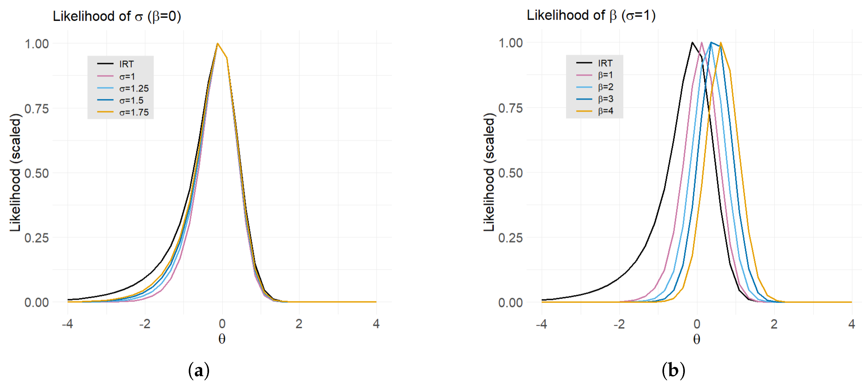
We aggregate their likelihood across all items in the construct through a summation of their item-level likelihoods. We are then able to observe how a student’s likelihood surface changes as we change the conditioning model by varying $\sigma$ and $\beta$. Figure 2 shows that as we increase $\sigma$, the surface becomes wider, and as we increase $\beta$, the distribution’s peak moves to the right. The black line represents the base likelihood of the student’s item responses without a conditioning model.

3.2.2. Estimating covariance terms, ${\sigma }_{ij}$

Once the convergence criteria have been met, the second step is to estimate the correlations between each pair of constructs. Each construct’s likelihood is evaluated at the same fixed nodes, thus for each node pair we evaluate the bivariate normal likelihood for the current value of ${\sigma }_{ij}$. The summation of these evaluations shown in Equation (9) becomes the objective function for the Newton optimization routine.

$$\begin{array}{cc}\hfill \mathsf{\ell }\left({\sigma }_{j{j}^{\prime }}\left|{\mathsf{\beta }}_j,{\mathsf{\beta }}_{j^{\prime }},{\sigma }_j,{\sigma }_{j^{\prime }};\mathit{w},\mathit{R},\mathit{X},\mathit{P}\right.\right)& =\sum _{i=1}^N{w}_i\log \left\{\int \int \frac{1}{2\pi \sqrt{\left|{\Sigma }_{\left(j{j}^{\prime }\right)}\right|}}exp\left({\widehat{\mathsf{ϵ}}}_{j{j}^{\prime }}^T{\Sigma }_{\left(j{j}^{\prime }\right)}^{-1}{\widehat{\mathsf{ϵ}}}_{j{j}^{\prime }}\right)\right.\hfill \\ \hfill & \phantom{=}\left.\times \left[\prod _{h=1}^{H_j}\mathrm{Pr}\left({\mathit{R}}_{ijh}\right|{\theta }_j,{\mathit{P}}_{h^{\prime }})\right]\left[\prod _{h^{\prime }=1}^{H_{j^{\prime }}}\mathrm{Pr}\left({\mathit{R}}_{i{j}^{\prime }{h}^{\prime }}\right|{\theta }_{j^{\prime }},{\mathit{P}}_{h^{\prime }})\right]\right\}d{\theta }_{j}d{\theta }_{j^{\prime }}.\hfill \end{array}$$

(9)

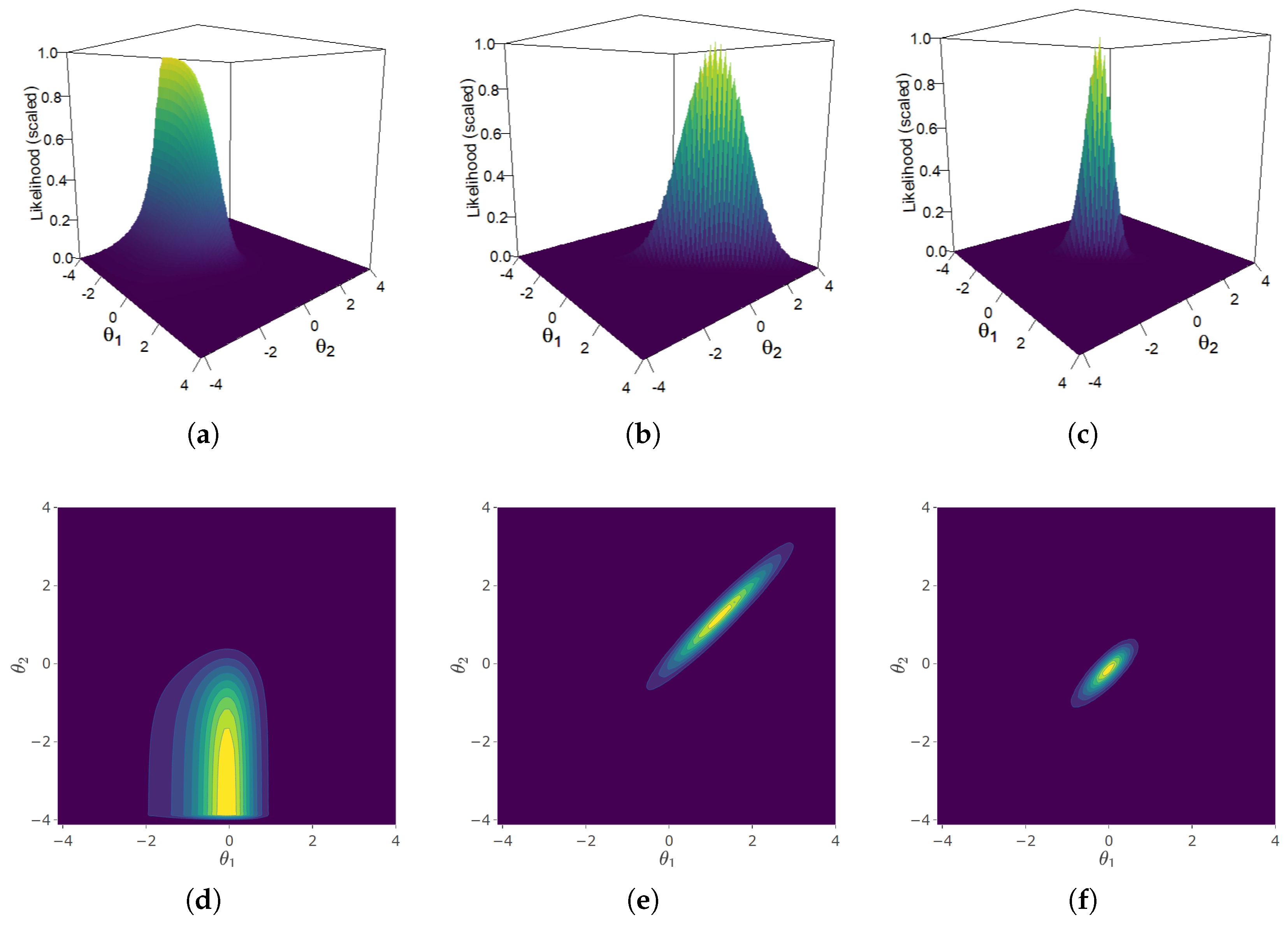
For any fixed n, this corresponds to a single student’s likelihood. We take the same student whose likelihood surface we examined previously on the Algebra subscale and now consider their composite likelihood, comprised of the Algebra and Geometry subscales. Figure 3 shows (a) the item response likelihood across the two constructs, (b) the likelihood of the student’s latent trait, and (c) the product of (a) and (b), where (c) is the function we seek to maximize, as a function of ${\sigma }_{i,j}$, holding ${\mathsf{\beta }}_{\mathit{i}}$, ${\sigma }_i^2$, ${\mathsf{\beta }}_{\mathit{j}}$, ${\sigma }_j^2$ all fixed. The figure shows that the student’s total likelihood, being the product of a normal distribution and an IRT model, also appears approximately normal. This is the posterior distribution of the latent trait, ${\theta }_i$, and will be relevant later for estimating group statistics.

Contrary to the procedure of the AM software [13], Dire optimizes ${\sigma }_{ij}$ by optimizing the correlation, r, in the Fisher Z space [Since variance terms have already been estimated at this stage, the covariance can be obtained by optimizing the correlation and calculating ${\sigma }_{ij}=r{\sigma }_{ii}{\sigma }_{jj}$]. This is a transformation defined by

$$\begin{array}{c}\hfill z=\frac{1}{2}ln\left(\frac{1+r}{1-r}\right)=arctanh\left(r\right),\end{array}$$

(10)

where r is the current value of the correlation. The benefit of optimizing in this space is that it maps the (−1,1) interval of a correlation to the real number line and consequently does not have to deal with proposed Newton steps outside of the allowable bounds. This allows for better handling and estimation of correlations between highly correlated constructs.

Though this procedure circumvents scenarios that would impede the optimization routine, it does not address the challenge of accurately estimating high correlations. When constructs are highly correlated, we observe that evaluation at subsequent node pairs may produce drastically different likelihoods. The true parameter value can “fall through the cracks”, and we are left with a biased estimate of the correlation.

One solution would be to evaluate the likelihood surface over a finer grid (i.e., significantly increase the number of nodes), but this quickly becomes computationally burdensome as the size of the data increases. Dire introduces a novel solution for accurately estimating correlations that relies on spline interpolation of the likelihood surfaces. Consider the Gaussian densities in Figure 3—the narrow, elongated shape suggests that the algebra and geometry constructs are highly correlated for this student. 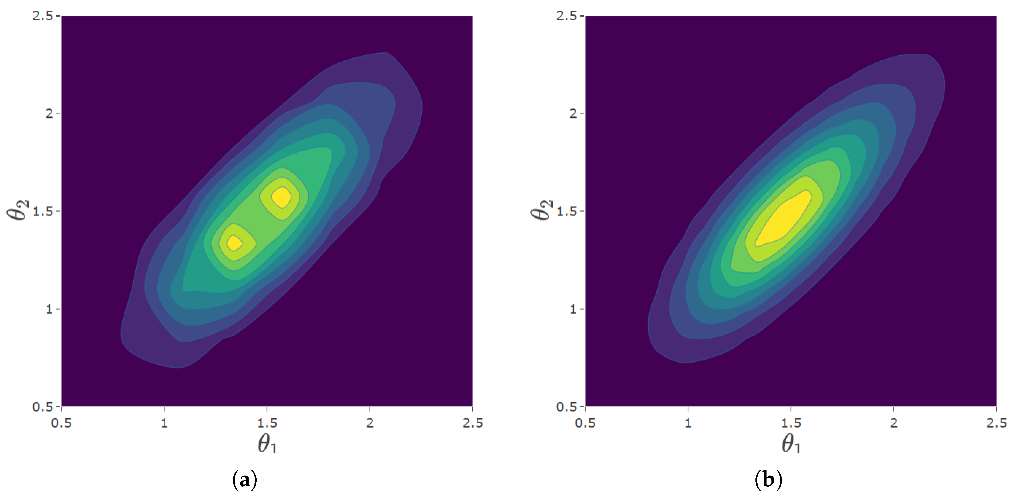In Figure 4, we compare a student’s likelihood using the standard grid and the grid produced with a cubic spline interpolation of the likelihood surface. The approximation of the likelihood surface using the standard grid is subject to discontinuities that are not real but the result of discretization.

Table 1. Correlation estimates and computing times.

Method	$\widehat{\mathit{\rho }}$	Log-Likelihood	Computing Time
Standard grid, Q = 34	0.995	−250,553.4	44 s
Spline interpolated grid, Q = 34	0.962	−252,857.9	119 s
Standard grid, Q = 136	0.961	−252,829.1	381 s

shows the estimated correlation, log-likelihood, and computing time for a variety of methods. The inefficacy of the standard grid becomes apparent, as we see the extent to which the estimated likelihood differs depending on the number of nodes. The spline interpolated grid requires greater computation time than the standard grid for a set value of q, but the relative improvement in estimation justifies its use. Spline interpolation results in nearly the same estimated correlation as if we had used 4x the number of nodes, at roughly a quarter of the computing time.

3.3. Variance Estimation

Dire estimates the variances of $\mathsf{\beta }$, as well as the residual variances (diagonal of the covariance matrix), using the cluster-robust (CR-0) method in Binder [26]. This method is also known as the Taylor Series Method, e.g., in Wolter’s survey sampling text [27]. These methods account for the weights and are cluster-robust in the sense of estimating arbitrary covariances between units within strata.

The Taylor series method involves estimating the variance for the set of parameters $\mathsf{\theta }$ using

$$\begin{array}{c}\hfill Var\left(\mathsf{\theta }\right)={\mathbf{d}}^{\prime }\widehat{\Sigma }\mathbf{d},\end{array}$$

(11)

where $\mathbf{d}$ is the vector of first derivatives of the score function with respect to the elements of $\mathsf{\theta }$ (and so has the same dimensions as $\mathsf{\theta }$), and $\widehat{\Sigma }$ is the estimated covariance term for $\mathsf{\theta }$. $\widehat{\Sigma }$ is obtained using survey sample methods for a two-stage sample, i.e.,:

$$\begin{array}{c}\hfill \widehat{\Sigma }=\sum _s\frac{P_s}{P_s-1}\sum _p^{P_s}({\mathbf{g}}_{sp}-{\overline{\mathbf{g}}}_s){({\mathbf{g}}_{sp}-{\overline{\mathbf{g}}}_s)}^{\prime },\end{array}$$

(12)

where s indexes the strata, and p indexes the PSUs in the strata, of which there are $P_s$ in the sth stratum. Here, the g terms are defined by

$$\begin{array}{c}\hfill {\mathbf{g}}_{sp}=\frac{\partial l_{sp}\left(\mathsf{\theta }\right)}{\partial \mathsf{\theta }},\end{array}$$

(13)

$$\begin{array}{c}\hfill {\overline{\mathbf{g}}}_s=\frac{1}{P_s}\sum _p^{P_s}\left({\mathbf{g}}_{sp}\right),\end{array}$$

(14)

where $l_{sp}$ is the log-likelihood function for only those units in stratum s in PSU p, evaluated at the estimated value for $\mathsf{\theta }$ (based on the full data).

The derivative vector ($\mathbf{d}$) can be calculated as the inverse Hessian of the likelihood function, or (assuming information equality [23]), as the sum of the stratum-level Jacobians of $\mathsf{\theta }$. The latter option is provided because it allows for replication of results from the AM software [13], but the former is recommended and is the default.

3.4. Plausible Values

Having estimated the model through MML as described in the preceding sections, we are able to draw plausible values for each student’s latent ability in these constructs through the following procedure:

• Holding $\Sigma$ fixed, draw $\tilde{\mathsf{\beta }}$ from a normal approximation to the posterior of $\mathsf{\beta }$
• Using the same $\Sigma$ and $\tilde{\mathsf{\beta }}$, compute the posterior distribution of ${\theta }_i$ for each student using the same quadrature nodes as in the initial optimization routine. Compute the mean and variance of each student’s posterior distribution as:

  $$\begin{array}{c}\hfill {\overline{\theta }}_i\approx \frac{{\sum }_{q=1}^Q{t}_q{l}_i\left(t_q\right)f\left(t_q;{\mathit{X}}_{\mathbf{i}}\tilde{\mathsf{\beta }},\Sigma \right)}{{\sum }_{q=1}^Q{l}_i\left(t_q\right)f\left(t_q;{\mathit{X}}_{\mathbf{i}}\tilde{\mathsf{\beta }},\Sigma \right)},\end{array}$$

  (15)

  $$\begin{array}{c}\hfill var\left({\theta }_i|\mathit{R},\mathit{X},\mathit{P},\tilde{\mathsf{\beta }},\Sigma \right)\approx \frac{{\sum }_{q=1}^Q{\left(t_q-{\overline{\theta }}_i\right)}^2{l}_i\left(t_q\right)f\left(t_q;{\mathit{X}}_{\mathbf{i}}\tilde{\mathsf{\beta }},\Sigma \right)}{{\sum }_{q=1}^Q{l}_i\left(t_q\right)f\left(t_q;{\mathit{X}}_{\mathbf{i}}\tilde{\mathsf{\beta }},\Sigma \right)},\end{array}$$

  (16)

  where $l_i\left(t_q\right)$ is the product of item response probabilities for individual i evaluated at node $t_q$.
• Using the mean and standard deviation from Step 2, randomly draw from a normal approximation to the posterior distribution.

This is straightforward in the case of a single construct. When there are multiple constructs, in addition to the posterior mean and variance for each individual construct, we compute posterior correlations between each pair of constructs in order to form the posterior covariance matrix, $\overline{{\Sigma }_i}$. Plausible values are then drawn from a multivariate normal approximation to the posterior with mean $\overline{{\theta }_i}$ and covariance matrix $\overline{{\Sigma }_i}$.

The normal approximation to the posterior distribution seems reasonable given Figure 3c,f and Figure 4b, each of which show approximately normally distributed looking surfaces, and both of which are based on published student data. More importantly, given Dire’s focus on LSA, this follows the methodology of NAEP and TIMSS [16,17].

Contrary to a standard Empirical Bayes (EB) approach, step (1) treats the population regression coefficients as random variables. EB does not fully account for the uncertainty in the modeled component and may result in biased statistics. By having a stochastic $\mathsf{\beta }$ we can integrate out this source of uncertainty. Once plausible values have been drawn, group level statistics may be calculated by first calculating the statistic for each of m plausible values. The average of these m estimates becomes the final estimate [28].

Plausible values are included in the data files provided by NCES, IEA, and OECD. As such, it only becomes necessary to draw new plausible values when there is a desire to estimate regression coefficients for variables that were not part of the conditioning model fit by these agencies. For a detailed discussion on the motivation and use of plausible values, see [1].

Having drawn plausible values, the user should use them according to Rubin’s rule [28], as explained in [29].

4. Examples

To analyze assessment data using the Dire package, the minimum necessary components are:

• Student data, including covariates (and weights, if applicable)
• Student item responses
• Item parameters
• Scaling information

These components are readily accessible and appropriately formatted for Dire out of the box when reading in data using the EdSurvey package. For users wishing to simulate some or all of this information, the lsasim R package provides a set of functions for simulating LSA data [30].

The following examples show (1) a general workflow of using Dire to estimate regression parameters and draw new plausible values using simulated data, and (2) how to use Dire with existing LSA data to address a particular research question.

4.1. Simulated Data

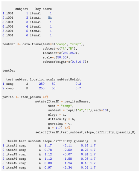
Using lsasim, we simulated background variables for 2000 students divided into 40 strata and 2 sampling units, as well as their responses to 20 dichotomous items divided into two subscales and the parameters for those items (see Appendix A).

To fit a latent regression model by marginal maximum likelihood, we call the function ‘Dire::mml’. The parameters to be specified are:

• formula: the model to be fit, expressed as Y   X1 + …+ XK
• stuItems: student item responses
• stuDat: student background variables, weights, and other sampling information
• idVar: student identifier variable in stuDat
• dichotParamTab: item parameters for dichotomous items
• polyParamTab: item parameters for polytomous items
• testScale: location, scale, and weights for each (sub)test
• strataVar: a variable in stuDat, indicating the stratum for each row
• PSUVar: a variable in stuDat, the primary sampling unit (PSU)

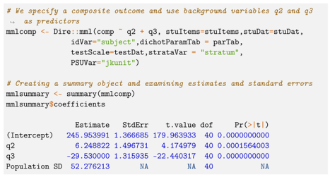
The general workflow is then straightforward. Once all necessary components are defined, the user need only determine the model they wish to fit. The outcome can be a single subscale (e.g., if one wished to estimate population parameters for Algebra proficiency), or it can be a composite of multiple subscales, such as in NAEP. Our simulated data contain two subscales, A and B, which we may fit a composite of.

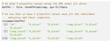
If one wished to make their simulated data available for secondary analyses, they may also wish to provide plausible values. This can be achieved using the ‘Dire::drawPVs’ function, which requires only a MML model object and a desired number of PVs to generate.

Consistent with IEA’s procedures in 2019 TIMSS, we draw five plausible values in this example [7]. Drawing more plausible values slows computation but always increases the accuracy of the estimates and variance estimates (Lou and Dimitrov [31] conclude, “The results indicate that 20 is the minimum number of plausible values required to obtain point estimates of the IRT ability parameter that are comparable to marginal maximum likelihood estimation(MMLE)/expected a posteriori (EAP) estimates”).

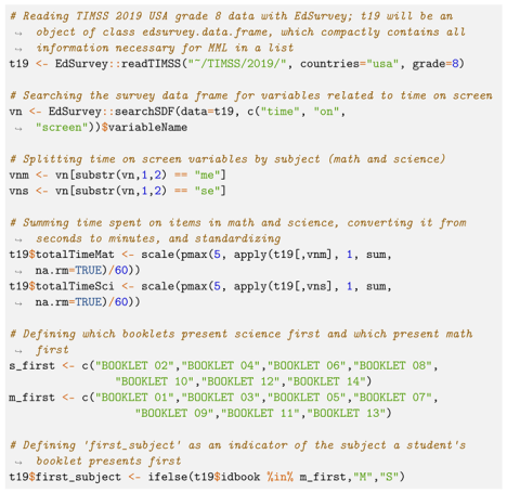
4.2. TIMSS Data

We used the international 2019 TIMSS U.S. Grade 8 data for this analysis, read in with the EdSurvey R package [(EdSurvey 4.0.1 CRAN: https://cran.r-project.org/web/packages/EdSurvey/index.html, GitHub: https://github.com/American-Institutes-for-Research/EdSurvey (accessed on 16 August 2023)]. These data bear information about how much screen time test takers spend on each item in the assessment, and these variables are not included in the conditioning model.

We first calculate each student’s total time (screen time, summed across all items) on math and science in minutes. Then we Z-scored these values. For TIMSS 2019 Grade 8 USA, with math achievement as our outcome, we consider a conditioning model with predictors of total time on the math blocks, total time on the science blocks, and which block students were exposed to first (math or science). Students are randomly assigned to one of 14 booklets, half of which present the science blocks first, and half of which present math first. Using this information, we created a binary variable equal to “M” if a student sees math first and “S” if they see science first, with “M” serving as the reference level. We additionally consider the two-way interactions of these predictors.

Notice that this is not intended to be a sophisticated look at mathematics screen time. A few issues arise, one being that students who see harder items may take longer to complete the items. For a more sophisticated approach to analyzing process data in this context, see [32,33]. However, the same criticism is not true of the time spent on science, since these items have no loading onto the mathematics test scores.

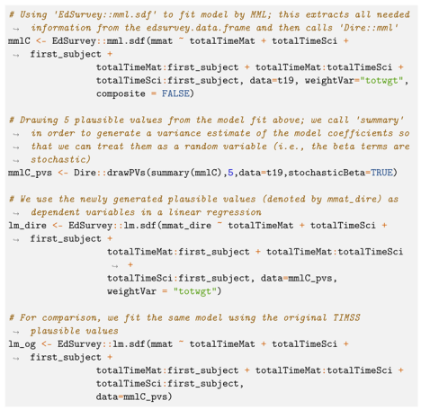
Having created the Z-scored time on assessment and first assessment (math or science) variables, we fit a new conditioning model using only the variables in our regression. We then drew plausible values from this conditioning model and fit a linear regression with these covariates to both the original and new plausible values. These plausible values could be used to fit models nested inside of the conditioning model, so if there are multiple regressions, the conditioning model could incorporate every covariate in them and then the plausible values could be used many times—as is typical of the plausible values that are provided on the original data [1].

We note that these models use “treatment coding”, so first_subject is 1 when the student takes science first and zero otherwise.

5. Results

Table 2. Summary of model; math achievement regressed on time spent on math, time spent on science, first subject seen, and their two-way interactions. *** p < 0.0001, ** p < 0.001.

	Estimate	SE	t-Value	dof	Pr(>|t|)
intercept	523.01	4.60	113.62	65.0	<$2.2\times {10}^{-16}$ ***
$Tim{e}_M$	13.95	3.79	3.68	23.3	0.0012 **$\phantom{*}$
$Tim{e}_S$	−2.84	4.35	−0.65	7.4	0.53 $\phantom{***}$
$Firs{t}_S$	16.73	2.72	6.16	22.1	$3.29\times {10}^{-6}$ ***
$Firs{t}_S\times Tim{e}_M$	41.83	5.3	7.97	28.0	$1.13\times {10}^{-8}$ ***
$Firs{t}_S\times Tim{e}_S$	−38.31	6.0	−6.42	14.1	$1.55\times {10}^{-5}$ ***
$Tim{e}_M\times Tim{e}_S$	−13.30	2.2	−5.97	11.8	$7.03\times {10}^{-5}$ ***

shows the summary results from fitting the MML model described above, i.e., with regression parameters obtained through direct estimation and standard errors obtained via the CR-0 method described in Section 3.3.

The estimated coefficient of 13.95 is the simple slope for time spent on math; that is, for a one standard deviation increase in time spent on math, the predicted scale score will increase by 13.95, assuming the student sees the math block first (i.e., $Firs{t}_s=0$) and spends an average amount of time on the science block (i.e., $Tim{e}_s=0$, since the times are standardized). These assumptions ($Firs{t}_s=0$, $Tim{e}_s=0$) are necessary because of the interaction terms—described below.

The estimated coefficient of −2.84 is the simple slope for time spent on science, implying that for a one standard deviation increase in time spent on science, the predicted scale score will decrease by −2.84. Here again, because of the interactions, we assume the math block is seen first, and that the student spends an average amount of time on the math block (i.e., $Tim{e}_m$ = 0).

The estimated coefficient of 16.73 for the first block seen implies that if a student spends an average amount of time on both the math and science blocks, seeing the science block first is associated with a predicted scale score increase of 16.73 points.

The estimated coefficient of 41.83 for the interaction of first block seen and time spent on math represents the change in slope of $Tim{e}_m$ when students see the science block first; that is, when a student sees science first, each one standard deviation increase in $Tim{e}_m$ is associated with an increase in predicted scale score of 13.95 + 41.83.

Similarly, the estimated coefficient of −38.31 for the interaction of first block seen and time spent on science represents the change in slope of $Tim{e}_s$ when students see the science block first. When a student sees science first, each one standard deviation increase in $Tim{e}_s$ is associated with a decrease in predicted scale score of −2.84–38.31.

Lastly, the estimated coefficient of −13.3 for the interaction of time spent on math and time spent on science represents the change in slope of $Tim{e}_m$ for a one standard deviation increase in time spent on science, and vice versa.

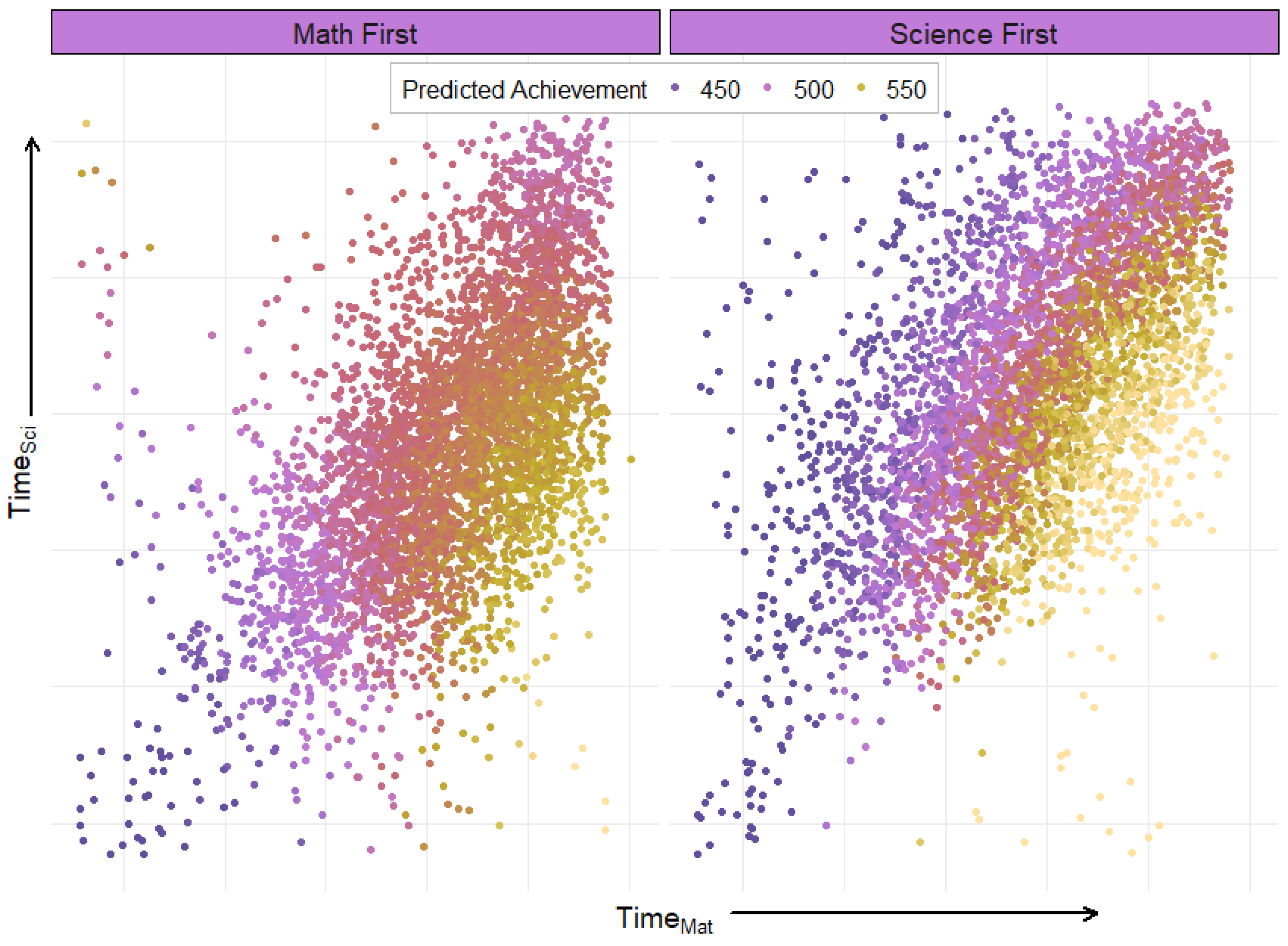
To aid the reader in understanding the net result of these interactions, Figure 5 shows predicted score as a function of time spent on math vs. time spent on science for students who saw math vs. science items first. Results are color-coded by predicted math achievement to demonstrate the association between time spent on the test and modeled score.

Taking all of the above into consideration, we expect the highest math achievement from a student who sees science first, spends a below average amount of time on science, and spends an above average amount of time on math. Likewise, we expect the lowest math achievement from a student who either sees math first and spends a below average amount of time on math and science items, or sees science first and spends an above average amount of time on science and a below average amount of time on math. A possible explanation could be that students seeing science first were better primed for the math items.

We draw five plausible values with this conditioning model, and then fit two linear regressions with the same variables used in the conditioning model: one using the original plausible values, and one using the newly generated ones.

Table 3. Linear regression models for math achievement using the original PVs ($R^2$ = 0.112) and new PVs ($R^2$ = 0.141). *** p < 0.0001, ** p < 0.001.

	Estimate	SE	t-Value	dof	Pr(>|t|)
Original PVs
intercept	518.68	4.98	104.17	60.9	<$2.2\times {10}^{-16}$ ***
$Tim{e}_M$	15.36	4.90	3.14	14.5	0.007 **$\phantom{*}$
$Tim{e}_S$	−2.54	4.49	−0.57	15.3	0.58 $\phantom{***}$
$Firs{t}_S$	22.19	3.38	6.57	18.0	$3.58\times {10}^{-6}$ ***
$Firs{t}_S\times Tim{e}_M$	31.93	5.60	5.70	36.0	$1.76\times {10}^{-6}$ ***
$Firs{t}_S\times Tim{e}_S$	−34.89	5.97	−5.84	25.2	$4.17\times {10}^{-6}$ ***
$Tim{e}_M\times Tim{e}_S$	−12.15	2.07	−5.87	16.7	$2.01\times {10}^{-5}$ ***
New PVs
intercept	523.06	4.19	124.71	93.8	<$2.2\times {10}^{-16}$ ***
$Tim{e}_M$	13.85	3.84	3.61	22.3	0.002 **$\phantom{*}$
$Tim{e}_S$	−3.20	3.14	−1.02	32.0	0.32 $\phantom{***}$
$Firs{t}_S$	16.63	2.86	5.81	24.8	$4.85\times {10}^{-6}$ ***
$Firs{t}_S\times Tim{e}_M$	42.07	4.57	9.21	63.6	$2.59\times {10}^{-13}$ ***
$Firs{t}_S\times Tim{e}_S$	−38.07	4.99	−7.63	48.6	$7.45\times {10}^{-10}$ ***
$Tim{e}_M\times Tim{e}_S$	−13.36	2.41	−5.54	15.0	$5.60\times {10}^{-5}$ ***

shows the results of these two models, and Figure 6 compares the estimates and standard errors.

6. Discussion and Conclusions

Understanding the population characteristics of student achievement is a complex task—especially when trying to augment existing surveys with additional data. Because the tests are designed to minimize response burden, they can only be used with a conditioning model (e.g., plausible values) to achieve an unbiased estimate. Further, a conditioning model must be fit that includes all variables of interest for the study. In our case, that is a new conditioning model because the process data variables are not included in the conditioning model.

NAEP and TIMSS each have plausible values made available to researchers for their analyses, but this places limitations on including external data or process data in the conditioning model. Dire enables users to use direct estimation, or simply fit a large conditioning model that includes external or process data variables. Once the conditioning model is fit, the user can draw new plausible values in order to have unbiased estimators of conditional statistics. Dire estimates the conditioning model efficiently by maximizing one subtest at a time (in the case of composite scores such as in NAEP or for TIMSS subtests). In addition, when the correlations are high it is often neceessary to use a higher density grid. To quickly calculate that, spline interpolation is applied, for accurate and fast estimation of correlations between subscales—this is novel in Dire and was used because the approximation was observed to be fast and accurate.

In our example, we fit a conditioning model with process data variables. We used direct estimation to estimate regression coefficients from an unbiased estimator. We then generated plausible values from that conditioning model and compared the results of a linear regression on the new plausible values that do include these variables to the original plausible values that do not. Setting aside the intercept, the estimated coefficients were further from zero (four of six cases), had smaller standard errors (five of six cases), larger degrees of freedom (five of six cases), and smaller p-values (four of six cases).

The model showed a surprisingly intricate association between time on tests and which test was first, with all interactions showing statistical significance and Figure 5 showing increases in total time (movement along the 45-degree line) being either non-linear (left plot: math first) or nearly unassociated with math score (right plot: science first).

We do not intend for these results on time spent on the exam to be a final word on the topic—they are merely presented as an example. In addition, screen time is not very informative, and does not add insight into what the student was doing. For example, a student who spends more time checking previous items is undertaking a very different activity than one who has the screen on one item with no clicks for an extended period. One hint is that there could be a “warm-up” effect, but this does not clarify why students who take more time on science after completing their math assessment have lower scores.