Radio Frequency Fingerprinting Authentication for IoT Networks Using Siamese Networks

Abstract

As IoT (internet of things) devices grow in prominence, safeguarding them from cyberattacks is becoming a pressing challenge. To bootstrap IoT security, device identification or authentication is crucial for establishing trusted connections among devices without prior trust. In this regard, radio frequency fingerprinting (RFF) is gaining attention because it is more efficient and requires fewer computational resources compared to resource-intensive cryptographic methods, such as digital signatures. RFF works by identifying unique manufacturing defects in the radio circuitry of IoT devices by analyzing over-the-air signals that embed these imperfections, allowing for the identification of the transmitting hardware. Recent studies on RFF often leverage advanced classification models, including classical machine learning techniques such as K-Nearest Neighbor (KNN) and Support Vector Machine (SVM), as well as modern deep learning architectures like Convolutional Neural Network (CNN). In particular, CNNs are well-suited as they use multidimensional mapping to detect and extract reliable fingerprints during the learning process. However, a significant limitation of these approaches is that they require large datasets and necessitate retraining when new devices not included in the initial training set are added. This retraining can cause service interruptions and is costly, especially in large-scale IoT networks. In this paper, we propose a novel solution to this problem: RFF using Siamese networks, which eliminates the need for retraining and allows for seamless authentication in IoT deployments. The proposed Siamese network is trained using in-phase and quadrature (I/Q) samples from 10 different Software-Defined Radios (SDRs). Additionally, we present a new algorithm, the Similarity-Based Embedding Classification (SBEC) for RFF. We present experimental results that demonstrate that the Siamese network effectively distinguishes between malicious and trusted devices with a remarkable 98% identification accuracy.

1. Introduction

The internet of things (IoT) refers to a network of billions of everyday devices (physical objects) equipped with sensors, software, and internet connectivity. The embedded sensors and internet connectivity transform these everyday objects into ‘smart’ devices by enabling them to collect and share data. IoT devices range from smart home gadgets like thermostats and TVs to more complex wearable healthcare technologies and self-driving cars [1,2,3,4]. The use cases for the IoT are limitless, and the rapid growth in technology continues to fuel more applications.

As the number of IoT devices continues to grow, cyberattacks targeting them can cause real-world catastrophic and life-threatening damage, extending beyond just the devices themselves. For example, if your smart toaster were compromised, it could malfunction or overheat, potentially causing a fire [5]. Many IoT devices lack robust security due to heterogeneous computing resources, diverse interfaces, and vulnerabilities introduced by different vendors or insecure supply chains. Moreover, most everyday users lack the technical expertise to configure or maintain strong security settings [6].

Cryptographic approaches for device authentication are computationally expensive, making them impractical for resource-constrained devices such as the IoT and Unmanned Aerial Vehicles (UAVs) [7]. Radio frequency fingerprinting (RFF) is a lightweight technique for authenticating devices that requires less computational power and energy, making it feasible to use in resource-constrained environments [8,9]. RFF is a technique that identifies transmitting devices by extracting unique signal features unintentionally introduced by hardware imperfections in their analog circuits. Even when devices are manufactured using the same electronic components and processes, they exhibit unique variations in the transmitted signal [10]. A transmitter radio typically includes an Analog-to-Digital Converter (ADC), Digital-to-Analog Converter (DAC), oscillators, power amplifiers, mixers, filters, etc. The imperfection produced includes nonlinearities in power amplifiers, phase noise in oscillators, and imbalance in the in-phase (I) and quadrature (Q) signals, serving as distinctive device-specific signatures. The use of machine learning (ML) and deep learning (DL) approaches like K-Nearest Neighbor (KNN), Support Vector Machine (SVM), and Convolutional Neural Network (CNN) has become very popular recently in extracting RF fingerprints of devices [11,12]. KNN classifies data points by comparing them with their closest neighbors and uses majority voting to make decisions [13]. SVM separates data into categories by finding an optimal boundary and maximizing the margin between classes [14]. CNNs are deep learning models designed to recognize patterns in structured data, such as images or signals, by extracting features layer by layer [15]. However, these models can only detect devices that were part of the initial training library [16,17,18]. If a new device not in the library needs to be detected, the model must be retrained from scratch, causing service disruption and making the approach expensive, in addition to scalability challenges. Also, these models need large datasets for training. For instance, research work in [19,20,21] uses data augmentation techniques to meet the large dataset requirement. In addition, these models struggle to detect rogue devices not involved in the (pre-deployment) training process. For example, [22,23] obtained low accuracy in detecting rogue devices that are not involved in the training process. To overcome these challenges, this research proposes the use of a Siamese network to extract embedded RF fingerprints. As explained in [24], Siamese networks compare the similarity between pairs of inputs, allowing the system to identify unknown (i.e., out-of-library) devices by measuring how closely their fingerprints match those of known devices. This approach minimizes the need for extensive retraining when new devices are added to the system and requires a relatively small training dataset as the model learns from input pairs rather than individual samples.

The key contributions of this paper are as follows:

• Extensive experiments using ten ADALM-PLUTO Software-Defined Radios (SDRs) collected from 19,920 frames, each containing 72 I/Q samples in the header and 1728 I/Q samples in the payload. The dataset is made publicly available through a GitHub repository (https://github.com/rajudhakal1/Adalm-Pluto-RF-fingerprinting-dataset, acceessed on 17 August 2025).
• The Siamese network was adapted and trained with I/Q samples from seven ADALM-PLUTO devices using data from two devices: one as an unknown device and the other as a validation device.
• A novel algorithm called Similarity-Based Embedding Classification (SBEC) was developed to identify both in-library and out-of-library devices, and its performance was evaluated using a real-world dataset collected from SDRs.
• SBEC can identify in-library and out-of-library devices with an impressive accuracy of approximately 98%.

The rest of this article is structured as follows: Section 2 discusses the recent developments in RF fingerprinting. Section 3 explains the processes of generation, transmission, reception, and collection of signals from the transmitter. Section 4 describes the datasets, base CNN model, Siamese network, and proposed SBEC. In addition, Section 5 illustrates the performance of the proposed approach. Section 6 presents the limitations of the work and future enhancements that can be conducted further. Finally, Section 7 concludes the paper.

2. Related Work

With the proliferation of wireless communication, the need for robust and efficient device authentication methods has become increasingly important. There has been growing interest in leveraging deep learning (DL) techniques for identifying devices through RF fingerprinting. Several studies have highlighted the effectiveness and precision of DL methods, especially with the evolution of cutting-edge technologies like Convolutional Neural Networks (CNNs) and Recurrent Neural Networks (RNNs), which have illustrated significant success in transmitter fingerprint identification. This section reviews some of the key recent works in this domain, demonstrating how DL continues to push the boundaries of RF fingerprinting for enhanced security and scalability.

The deep learning techniques discussed by Jian et al. in [17] focus on Convolutional Neural Networks (CNNs) for RF fingerprinting to determine the unique characteristics of over 10,000 radio devices. The study evaluated the performance and scalability of different CNN architectures, including a custom baseline model and a modified ResNet-50-1D. The experiments, performed on Wi-Fi and Automatic Dependent Surveillance-Broadcast (ADS-B) signals, consider different factors like the number of devices, the size of the training dataset, channel conditions, and signal-to-noise ratio (SNR). Out of them, ADS-B provides higher accuracy and is easier for classification. However, this approach is unable to detect new devices without retraining. Furthermore, the computational overhead for scaling to those devices increases as the number of devices increases. This leads to the need for more efficient and scalable methods.

The study performed by Kandel et al. [16] utilized channel state information, where the phase differences of RF chains are employed in Multiple-Input/Multiple-Output (MIMO) systems for creating distinct device fingerprints. This work utilized 17 identical network interface cards (NICs) in both static and mobile indoor environments, including hallways and small office rooms, under non-line-of-sight conditions, achieving device identification accuracy of 97% and 92%, respectively. However, the model has the limitation of identifying outliers. In addition, the method struggled to handle new devices without retraining, limiting its relevancy in dynamic large-scale networks.

In RF fingerprinting, a few-shot learning model, FSig-Net was proposed by Zhao et al. [18] based on deep metric learning to enhance recognition performance in cases where signal samples are limited. FSig-Net provides hardware-specific discrepancies in wireless devices, showing a unique layer of security that cannot be replicated by third parties. By learning similarity measures between features, the model reduces its reliance on large datasets and avoids the constraints of fixed distance metrics. The approach was tested on eight mobile phones and eighteen IoT devices, acquiring recognition accuracies of 98.28% for mobile phones and 98.20% for IoT devices with as few as ten samples per class.

However, while FSig-Net outperforms traditional deep learning methods in high signal-to-noise ratio (SNR) environments, its effectiveness is reduced in low-SNR conditions. The model also faces challenges when dealing with noisy or overlapping signals, limiting its robustness in real-world applications. There is a need to enhance FSig-Net’s performance in low-SNR settings to improve generalization and recognition accuracy, particularly when training samples are limited.

An RF fingerprinting approach proposed by Soltani et al. [19] uses a neural network to identify UAVs by learning subtle imperfections in their transmitted waveforms. Their multi-classifier technique, combined with RF data augmentation, enhanced the system’s ability to detect both known and new UAVs, achieving an overall classification accuracy of 99%. This method significantly improved classification accuracy compared to a single-classifier approach. However, it relies heavily on extensive data augmentation and lacks flexibility in handling new devices, necessitating substantial retraining to incorporate new devices into the system. Several studies have been conducted to determine new devices using Convolutional Neural Networks [25,26,27,28,29,30,31,32], with a focus on RF fingerprinting. However, they lack the scalability to adequately add new devices. In addition, models need to be retrained from scratch after a new device is added to the system. In the analysis by Otto et al. [33], Support Vector Machines (SVMs) and Convolutional Neural Networks (CNNs) were used for identifying wireless devices. The CNNs achieved better accuracy at classifying data, although the SVMs were computationally more efficient, particularly in training and inference times. However, both methods have certain shortcomings, particularly in the case of handling new devices and detecting outliers. As new devices are deployed, the need for extensive retraining decreases scalability and practicality in dynamic environments. Therefore, this highlights the need for new methods that ensure robustness and scalability, especially in detecting new devices not involved in the training process.

Nowadays, RF fingerprinting has evolved from traditional machine learning to a deep learning architecture. A study conducted by Morge-Rollet et al. [34] on RF fingerprinting used a Siamese network. In this approach, I/Q samples collected from 16 identical USRPX310 Software-Defined Radios (SDRs) in two configurations, over the air and a cable, were analyzed, resulting in an accuracy of 99%. This method needs minimal data for device identification by processing I/Q signals and applying one-shot learning. However, this work is limited to binary classification and is limited to training and testing the Siamese network with the same and different inputs.

Another approach proposed by Alhoraibi et al. [35] analyzes machine learning (ML) and deep learning (DL) algorithms for physical-layer authentication (PLA) in wireless networks. The signal classification and specific emitter identification are achieved using algorithms like Random Forest and Support Vector Machine (SVM). Furthermore, deep learning techniques such as Convolutional Neural Networks (CNNs) and Autoencoders are utilized to handle high-dimensional data and model complex relationships. RFF is extracted from channel-based features, such as Received Signal Strength (RSS) and channel state information (CSI). Despite their effectiveness, these methods encounter limitations like computational challenges and poor scalability when adding new devices. In addition, they do not explore how to detect rogue devices not involved in the training process.

A significant advancement in signal classification was presented by Langford et al. [36] for applying Siamese networks in RFF. Addressing the data limitations regarding traditional deep learning methods like CNNs, which typically require large datasets and frequent retraining, this method demonstrated that Siamese networks could effectively distinguish between similar and dissimilar signals, even in scenarios with limited data. However, their approach cannot detect new devices not involved in the training process. Additionally, the study primarily focused on binary classification tasks. It did not extend to multi-class classification or outlier detection, both of which are crucial for practical RFF in dynamic environments.

In addition, the investigation by Meng et al. [37] applied a Siamese network for device identification in few-shot scenarios for LoRa devices. A simulated attack detection method was employed in such a way that only legitimate devices were used in the support set, which further led to an improvement in the classification accuracy of 90%. However, this approach struggles in extreme low-shot settings, with reduced accuracy for one-shot and three-shot scenarios. Here, the one-shot setting refers to pulling out one reference sample from each known class for comparison with the sample to be tested, and the low-shot setting means a lower number of reference samples from each known class. Also, the accuracy decreases under low-signal-to-noise ratio conditions.

The recent advancements in RF transmitter identification present challenges in differentiating between known and unknown transmitters in complex electromagnetic environments. One of the studies proposed by Guomin Sun [38] employed combined Siamese networks for transmitter identification (CSNTI) to identify twelve radio devices (eight known and four unknown) with I/Q samples captured by NI USRP-2974. From the series of Siamese network classifiers, each classifier distinguishes one transmitter from the others. The output is normalized using a softmax function. An accuracy of 87% was obtained for identifying known devices and detecting unknown devices. However, this system is not robust enough to handle the increased number of transmitters. For example, if we have 100 known devices, we must train 100 Siamese network classifiers. As a result of this, the computational complexity increases. The model needs to be retrained to add new devices by increasing the number of classifiers each time.

Upon a comprehensive review of the recent advancements in RF fingerprinting, we found that CNNs are predominantly employed to capture subtle variations in device fingerprints. Although CNNs are effective, these models require retraining whenever new devices are introduced, limiting their scalability. The research community for RF fingerprinting is increasingly exploring Siamese networks. However, these efforts often overlook the crucial aspect of distinguishing between known devices and identifying outliers. To address these challenges, we propose a novel approach utilizing Siamese networks to recognize known devices while effectively detecting outliers, thereby enhancing the system’s ability to adapt to new devices without extensive retraining and improving its robustness and scalability in a changing environment.

3. Background

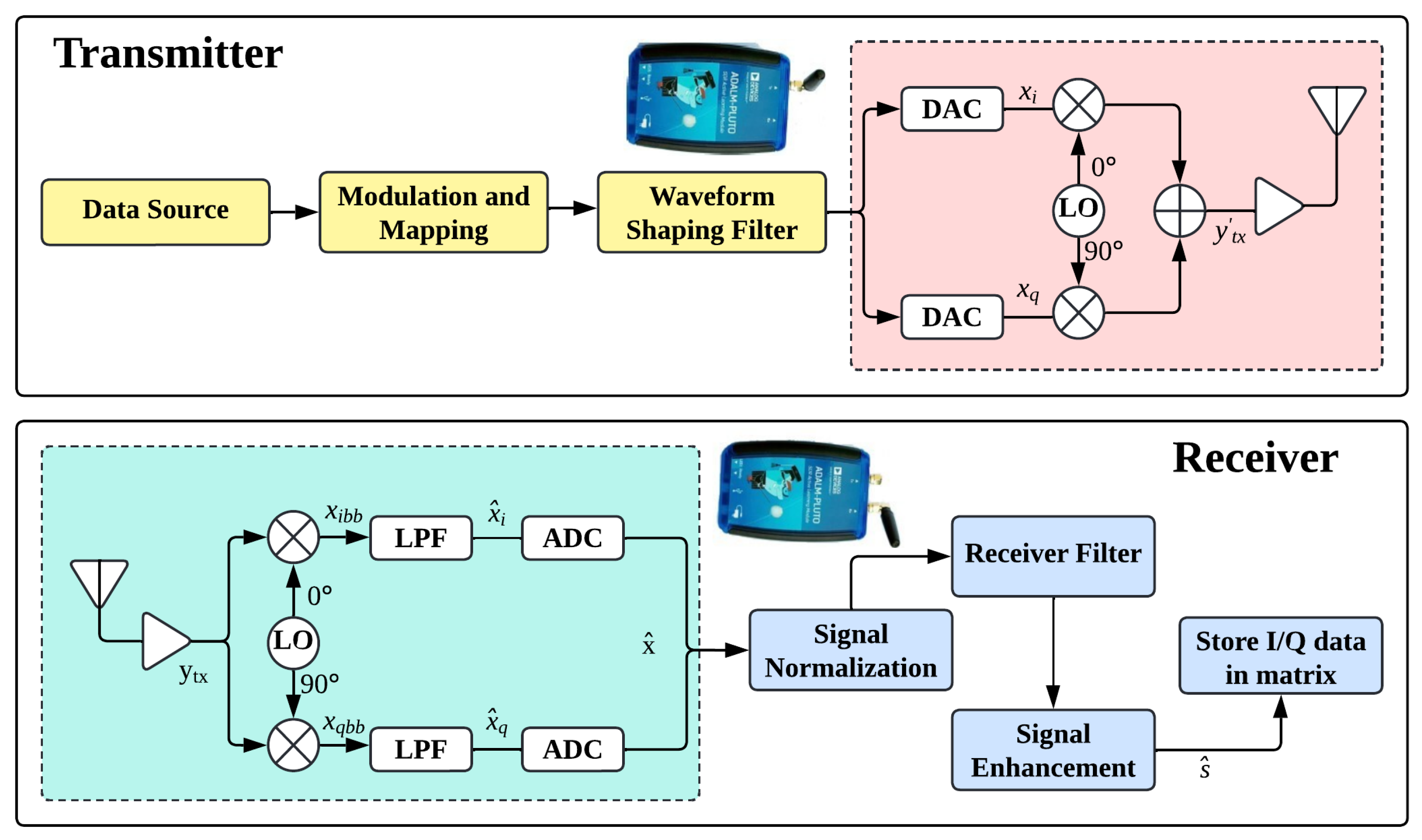
Figure 1 shows a block diagram of a general single-carrier transceiver system consisting of transmitter and receiver systems. The local oscillator (LO) generates a pair of orthogonal sine and cosine carrier waves. During transmission, these orthogonal waves convert the in-phase (I) and quadrature (Q) baseband signals to the passband. In contrast, at the receiver, they convert the received passband signal back to the baseband. Ideally, the LO at both transmitter and receiver should be perfectly synchronized in frequency and phase. In practice, however, small hardware variations cause mismatches, resulting in carrier frequency offset (CFO), carrier phase offset (CPO), and IQ imbalance. Similarly, the Analog-to-Digital Converter (ADC) and Digital-to-Analog Converter (DAC) at the transmitter and receiver are not perfectly synchronized, starting sampling at slightly different times, which leads to sampling frequency offset (SFO). Packet detection at the receiver may also be offset by some samples, producing packet boundary detection errors [39]. The magnitude and combination of these imperfections are determined by manufacturing tolerances, component aging, and environmental factors, which vary slightly from one transmitter to another. As a result, each device imprints a distinctive and stable distortion pattern onto its transmitted I/Q samples—its radio frequency fingerprint. RF fingerprinting algorithms exploit these device-specific signatures as unique identifiers and provide an additional layer of authentication in wireless communication systems. Next, we show the mathematical representation of the transmission and reception of a signal.

3.1. Transmitter-Side Signal Modeling

The continuous baseband I and Q signals on the transmitting side are denoted as $x_i\left(t\right)$ and $x_q\left(t\right)$, respectively. The ideal bandpass signal generated by the transmitter can be expressed as

$$y_{tx}\left(t\right)=\Re \left\{x\left(t\right)e^{j2\pi f_{c}t}\right\}=x_i\left(t\right)cos\left(2\pi f_{c}t\right)-x_q\left(t\right)sin\left(2\pi f_{c}t\right)$$

(1)

where $f_c$ is the carrier frequency that the LO generates. However, the I and Q branch signals suffer from unequal carrier amplitude and phase due to IQ imbalance. Considering the signal from the I channel as the reference, $\alpha$ represents the relative amplitude gain of the Q signal, and $\varphi$ indicates the relative phase difference between the I and Q signals. As a result, the transmitter’s imbalanced RF bandpass signal is expressed as

$${\tilde{y}}_{tx}\left(t\right)=x_i\left(t\right)cos\left(2\pi f_{c}t\right)-\alpha x_q\left(t\right)sin(2\pi f_{c}t+\varphi )$$

(2)

3.2. Receiver-Side Signal Modeling

The transmitted signal propagates through a channel with impulse response $h\left(t\right)$, and the received signal is affected by noise $n\left(t\right)$. Assuming an ideal channel $h\left(t\right)=1$, the received signal simplifies to

$$y_{rx}\left(t\right)={\tilde{y}}_{tx}\left(t\right)+n\left(t\right)$$

(3)

Substituting ${\tilde{y}}_{tx}\left(t\right)$ from Equation (2), the received signal can be expressed as

$$y_{rx}\left(t\right)=x_i\left(t\right)cos\left(2\pi f_{c}t\right)-\alpha x_q\left(t\right)sin(2\pi f_{c}t+\varphi )+n\left(t\right)$$

(4)

For simplicity, noise $n\left(t\right)$ is ignored in theoretical derivations. After mixing with the LO signals, the I and Q baseband components are extracted as follows:

$${\widehat{x}}_i\left(t\right)={\displaystyle \frac{x_i\left(t\right)}{2}}cos(2\pi \delta ft-\theta )-{\displaystyle \frac{\alpha x_q\left(t\right)}{2}}sin(2\pi \delta ft+\varphi -\theta ),$$

(5)

$${\widehat{x}}_q\left(t\right)={\displaystyle \frac{\beta x_i\left(t\right)}{2}}sin(2\pi \delta ft-\psi -\theta )-{\displaystyle \frac{\alpha \beta x_q\left(t\right)}{2}}cos(2\pi \delta ft+\varphi -\psi -\theta ),$$

(6)

Here, $\delta f$ is the carrier frequency offset (CFO) between the transmitter and receiver local oscillators, $\theta$ is the phase offset from the receiver’s local oscillator during downconversion, $\beta$ is the amplitude gain mismatch in the receiver’s I branch relative to the Q branch, and $\psi$ is the phase mismatch between the I and Q branches in the receiver. Finally, the discrete baseband signal is given as

$$\widehat{s}\left[k\right]={\widehat{x}}_i\left(k{T}_s\right)-j{\widehat{x}}_q\left(k{T}_s\right),$$

(7)

Here, ${\widehat{x}}_i\left(k{T}_s\right)$ and ${\widehat{x}}_q\left(k{T}_s\right)$ are the sampled I and Q components, and $T_s$ is the sampling period, given by $T_s=1/f_s$, where $f_s$ is the sampling rate. All Equations (1)–(7) are adapted from the signal modeling approach presented in [40].

3.3. I/Q Data Storage and Formatting

The received I/Q data is put into a structured format to be stored and analyzed further. This is conducted after preprocessing steps, compensating for unwanted impairments like CFO, CPO, DC offset, and timing clock skew. As shown in Equation (7), the I and Q components are the real and imaginary parts of the preprocessed signal $\widehat{s}\left[k\right]$. They are taken out and put into a 4D matrix with dimensions [$k\times 2\times 1\times \mathtt{total}\_\mathtt{frames}]$. Here, k corresponds to the frame length (i.e., the number of samples per frame), 2 represents the I and Q components, 1 represents a single data stream, and total_frames means the total number of frames captured. Finally, the matrices obtained from each device are saved in separate files to be used for the RF fingerprinting task.

3.4. System Model

Figure 2 illustrates the system model for training and testing the Siamese network. First, seven devices, i.e., devices 1–2 and 5–9, are considered known or in-library, and two devices, i.e., devices 3–4, are unknown or out-of-library devices. For training purposes, only data from in-library devices is used. The remaining device 10 is being used for validation purposes, which we will discuss later. From in-library devices, the data is split into training, testing, and validation sets in the proportion of 7:2:1. Data pairs are generated from training sets, creating positive and negative pairs. Positive pairs are created by randomly selecting two samples from the same class. Negative pairs are generated by selecting one sample from a particular class and another from the other six remaining classes. For similar samples (from the same class), a label of 1 is assigned, while pairs of dissimilar samples (from different classes) are assigned a label of 0. These data pairs train the Siamese network with a contrastive loss function described in Section 4.4.

The test dataset comprises 20% data from known devices (devices 1–2 and devices 5–9) and all data from unknown devices (devices 3–4) and is used to evaluate trained Siamese networks. The SBEC algorithm described in Section 4.5 is used to detect unknown devices and identify known devices.

4. Methodology

This section explains the data collection process, presents the Siamese network model implementation with the CNN base model, and outlines the workings of the SBEC algorithm for identifying known and unknown IoT devices.

4.1. ADALM-PLUTO Dataset

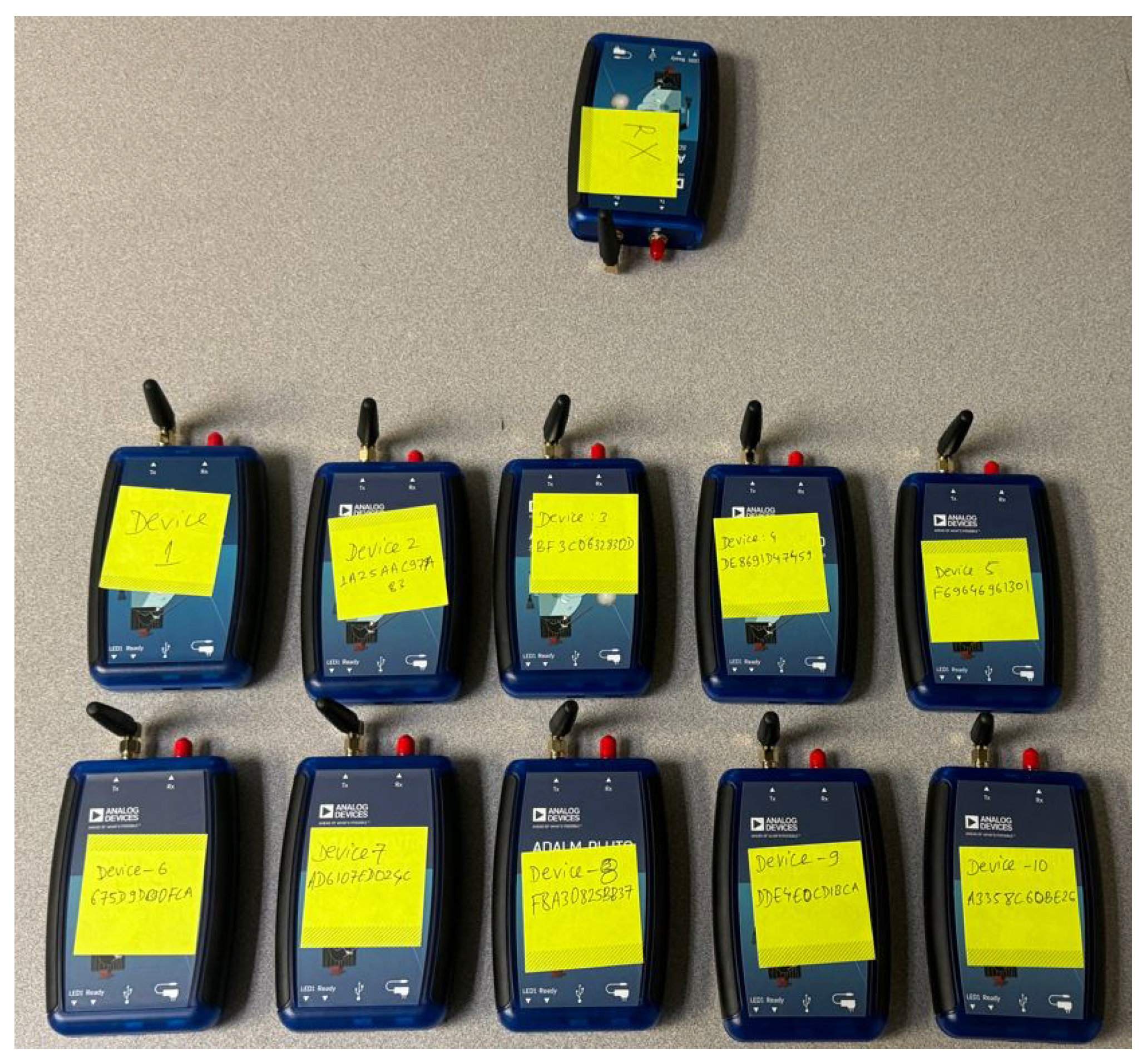
The data collection process involves 11 different ADALM-PLUTO Software-Defined Radios (SDRs) (see Figure 3) programmed and controlled via MATLAB R2024b. One ADALM-PLUTO functions as the receiver (RX), capturing the in-phase (I) and quadrature (Q) signal components transmitted by the remaining 10 TX SDRs. The TX transmits real-time Orthogonal Frequency Division Multiplexing (OFDM) signals. All data collection was conducted in an indoor office room with approximate dimensions of 6 feet width by 15 feet length. The TX and RX PLUTO devices were positioned in fixed locations, approximately 5 feet apart. Importantly, no surrounding wireless devices or access points were deliberately turned off during data collection. Wi-Fi routers, mobile phones, and other typical wireless sources in the lab environment remained operational, providing a realistic level of interference.

The transmitting and receiving devices were configured with a 128-point FFT, a 32-point cyclic prefix, 72 active subcarriers, 30 kHz subcarrier spacing, and a channel bandwidth of 1 MHz. After each nine subcarriers, a pilot signal was inserted to correct the phase at the receiving end. Each frame transmitted consisted of a synchronization signal generated using a Zadoff–Chu sequence, followed by a reference symbol for channel estimation. The header was encoded with BPSK at a 1/2 rate for robustness, followed by 30 QPSK-modulated data symbols encoded with convolutional coding at a 1/2 rate. There were null carriers at the DC and band edges to confine the spectral emissions. A carrier frequency of 1 GHz was used to mimic IoT nodes. The transmitter and receiver PLUTOs was set to 60 dB and 71 dB, respectively. Frames were repeated and buffered to meet the PLUTO hardware’s minimum waveform size requirement. The system performs synchronization, FFT demodulation, frequency offset correction, and signal decoding at the receiving end. The decoded and known transmitted header bits were compared using MATLAB’s comm.ErrorRate function. Overall Bit Error Rate (BER) was zero for each transmission for the collected data. From each TX device, 19,920 frames were collected, each consisting of 72 header I/Q samples and 1728 payload I/Q samples. Fingerprints were extracted exclusively from the header as it is well-suited for capturing hardware-specific imperfections.

Table 1. Parameters for OFDM transmission and reception.

Parameter	Value	Parameter	Value
FFT Length	128	Cyclic Prefix Length	32
Number of Subcarriers	72	Subcarrier Spacing	30 KHz
Channel Bandwidth	3 MHz	Pilot Subcarrier Spacing	9
Header Modulation	2 (BPSK)	Payload Modulation	4 (QPSK)
Coding Rate	1/2	Symbols per Frame	30
Frames Transmitted	19,920	Sample Rate	3.84 MHz
Tx Center Frequency	1 GHz	Rx Center Frequency	1 GHz
Transmit Gain	60 dB	Receive Gain	71 dB
Frames per device	19,920	Samples per frame in header	72
Samples per frame in payload	1728	Number of transmitters	10

summarizes the parameters used for the transmission and reception process.

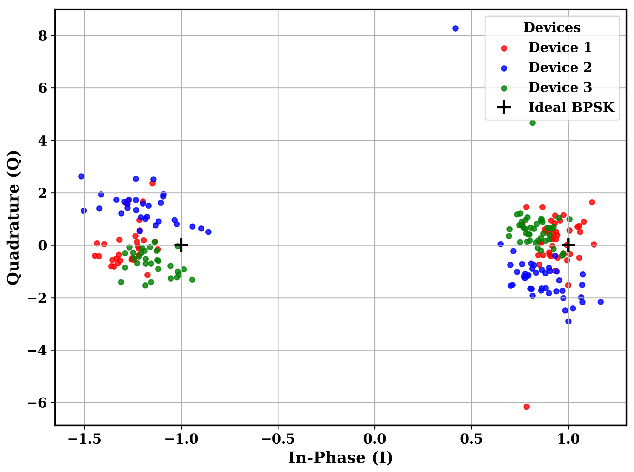
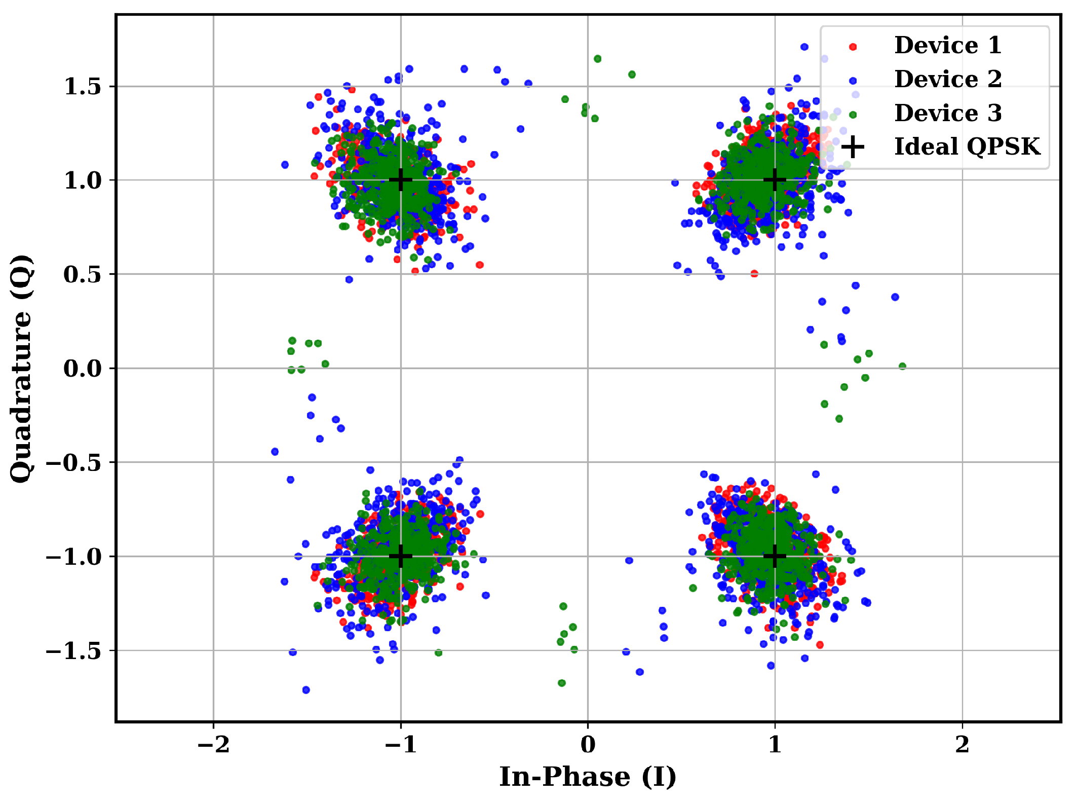
Figure 4 and Figure 5 show the I/Q scatterplots of the header and payload, respectively, of one single frame each from 3 devices, i.e., devices 1, 2, and 3. We can observe that each of the I/Q samples is deviated from the ideal point and shows minute variations among different devices, which represent the RF signatures of each device.

Figure 6 and Figure 7 show the histograms of the Probability Density Functions (PDFs) of header samples of all ten devices for I and Q components, respectively. We can observe variations in IQ signals among different devices, but the variations are minute.

In our actual implementation, we merge 10 consecutive frames to form a single frame, effectively increasing the feature space from 72 to 720 I/Q samples. This was necessary because the original header size of 72 was too short to capture meaningful RF fingerprints. Thus, the performance of our Siamese network improved significantly. After merging, each device ends up with 1992 frames, where each frame contains 720 I/Q samples, making the feature extraction more robust.

4.2. Base Model for Siamese Network

The CNN structure that acts as the base of the Siamese network is shown in Figure 8. The input layer is of size (frame_length, 2) and is followed by the batch normalization layer that standardizes the data. I and Q samples from each frame are arranged in the size of [frame_length, 2], where each row represents samples, and the two columns represent I and Q samples. For example, in the header part of our ADALM-PLUTO dataset, the frame_length is 72. Then, zero padding of size two is used after the input layer to preserve the edge for successive convolution layers. The architecture has four convolutional layers, each followed by RELU activation functions and max pooling layers for dimension reduction. The first two convolutional layers contain 64 filters with sizes of 2 and 4, respectively. The subsequent two layers each have 32 filters, with sizes of 16 and 32. A flattening layer follows these layers to prepare the data for the dense layer, which has 256 neurons and uses a sigmoid activation function. The final output layer also has 256 units. The hyperparameters for our model are adapted from the work of [41].

4.3. Siamese Network

The structure of the Siamese network is shown in Figure 9. Two identical CNNs take two inputs. Two outputs from two networks are used to calculate the Manhattan or L1 distance between them, called the similarity score of the given two inputs. The formula in Equation (8) is used to calculate the L1 distance [42]. The Siamese network is trained so that similar inputs yield output one, and different inputs generate output zero.

$$d({\mathbf{f}}_1,{\mathbf{f}}_2)=\sum _{i=1}^r\left|f_{1,i}-f_{2,i}\right|$$

(8)

where

• ${\mathbf{f}}_1$ and ${\mathbf{f}}_2$ represent the outputs from the two CNNs;
• $d({\mathbf{f}}_1,{\mathbf{f}}_2)$ is the Manhattan or L1 distance between ${\mathbf{f}}_1$ and ${\mathbf{f}}_2$;
• The indices i range from 1 to r, where r is the dimensionality of the fingerprint vectors.

The outputs of the two CNNs in the Siamese network, i.e., ${\mathbf{f}}_1$ and ${\mathbf{f}}_2$, are feature vectors representing the unique characteristics of the two input samples. Each element of these vectors corresponds to a specific learned feature, capturing patterns or attributes within the signal that help to distinguish between different devices. These feature vectors are optimized to ensure that similar samples (from the same device) have closer values and dissimilar samples (from different devices) have more distinct values by using the contrastive loss function, as discussed in Section 4.4.

The Siamese network is applied in this work because it is well-suited for comparing pairs and distinguishing between similar (known) and dissimilar (unknown) devices. Its contrastive loss function minimizes the distance between similar pairs and maximizes it for dissimilar pairs, enhancing the model’s ability to differentiate devices effectively. Additionally, the Siamese network is adaptable to new devices without retraining as it only needs comparison to reference samples. By creating a compact embedding space where similar signals are close together, the network enables reliable identification based on signal similarity, making it an efficient solution for this problem.

4.4. Contrastive Loss

Contrastive loss functions are widely used in Siamese networks to learn embedding, where the goal is to have similar inputs produce outputs that are close to each other in the embedding space. In contrast, dissimilar inputs generate embeddings that are farther apart. An embedding in this context refers to the output produced by each of the CNNs in the Siamese network. The contrastive loss ensures that similar inputs remain close together in the embedding space, whereas dissimilar inputs are pushed further apart. To prepare the data for this process, pairs of inputs $(x_1,x_2)$ are labeled such that $y=1$ if the pairs come from the same device (similar pairs) and $y=0$ if they come from different devices (dissimilar pairs). The Siamese network, consisting of two identical CNNs, generates two embeddings: $f_1$ and $f_2$. The contrastive loss L is formulated by [43] as

$$L={\displaystyle \frac{1}{2}}\left(y·D^2+(1-y)·max{(0,m-D)}^2\right)$$

(9)

where $D=d({\mathbf{f}}_1,{\mathbf{f}}_2)$ is the L1 distance between the embeddings (refer to Equation (8)), and $m>0$ is a margin parameter that defines the minimum distance that should be maintained between dissimilar pairs.

This formulation has two cases:

• For similar pairs ($y=1$), the loss reduces to $L={\displaystyle \frac{1}{2}}{D}^2$, which penalizes the model when similar pairs are far apart, encouraging the network to bring their embeddings closer together.
• For dissimilar pairs ($y=0$), the loss becomes $L={\displaystyle \frac{1}{2}}max{(0,m-D)}^2$, which penalizes the model only when the distance between dissimilar pairs is less than the margin m. This pushes embeddings of dissimilar pairs at least m units apart in the learned space.

By jointly minimizing both components, the contrastive loss helps the network to learn an embedding space where similar pairs are mapped close together and a defined margin separates dissimilar pairs. This enhances the discriminative capability of the Siamese network, allowing for effective verification or identification of devices based on embedding similarity.

4.5. Similarity-Based Embedding Classification (SBEC)

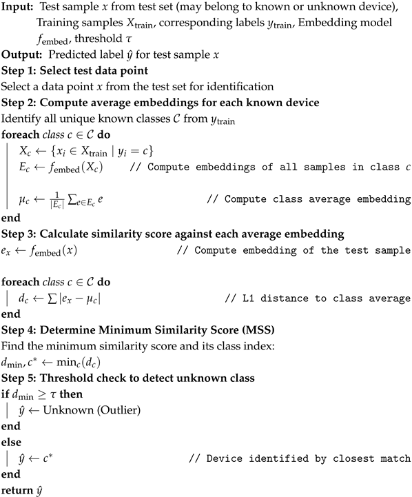
The SBEC shown in Algorithm 1 is used to identify known and unknown devices using the average embeddings of each in-library device. First, the average embedding for each of the known devices is calculated using data in the training set. For each data point from the test set, the similarity score is calculated against the average embeddings of each known device. The minimum among these similarity scores, i.e., minimum similarity score (MSS), and the corresponding labels of the known device are recorded. If the MSS exceeds the predefined threshold, the data point is classified as a fingerprint from an unknown device or outlier. If the minimum similarity score is less than the predefined threshold, the test data point is classified as the device corresponding to its index.

The existing device classification techniques, such as KNN, SVM, and CNN, are typically trained in a closed-set setting, allowing them to classify only devices that are included in the training set. To accommodate new devices, these techniques require complete retraining, making the system computationally expensive and impractical for dynamic IoT environments. In contrast, the proposed SBEC performs open-set classification by comparing the embedding of each sample with the average embedding of each known device. The existing works using Siamese networks [38,41,44,45] compare the sample to be tested with one randomly selected sample from each of the known devices. In contrast, our SBEC compares the embedding of the sample to be tested with the average embedding of each known device. Taking the average embedding from each known device, rather than selecting a single sample, enables the representation of the entire data distribution of the known devices rather than relying on just one individual sample.

Algorithm 1: Similarity-Based Embedding Classification (SBEC)

4.6. Threshold Calculation

Figure 10 demonstrates the steps involved in calculating the threshold using a validation set and the trained Siamese networks. First, we calculate the trained model embedding for each data point in the validation set. Then, the Manhattan distance between each of these embeddings is calculated against the average embeddings of each device from the training set, and the minimum distance, i.e., MSS, is recorded. Now, we have MSSs for known and unknown data points in the validation sets. The job is determining the threshold to differentiate between known and unknown devices. From the range of minimum and maximum MSS values, we selected 500 different threshold values in equal intervals and applied these thresholds to distinguish between known and unknown data points. The threshold value that provides the best f1-score value to differentiate between known and unknown devices is selected as the optimum threshold and applied in the SBEC algorithm. The validation data consists of 10% of data samples from each known device and all data from the device assigned as the validation device.

5. Results and Discussion

This section describes the performance of the proposed Siamese network in detecting and identifying known and unknown devices.

5.1. Siamese Network Training and Learning Curve

Each device contains 19,920 raw frames, with 72 I/Q samples per frame. To expand the feature space, we merge every 10 consecutive frames into one, resulting in 1992 merged frames per device, each with 720 I/Q samples. For our experiment, devices 1–2 and 5–9 (a total of seven known devices) are combined into a single pool of 13,944 frames. This pool is shuffled randomly and split into 70% for training (9760 frames), 10% for validation (1394 frames), and 20% for testing (2790 frames). Device 10 is used exclusively for validation and contributes an additional 1992 frames, bringing the total validation set to 3386 frames. Devices 3 and 4 are treated as unknown (rogue) and contribute 3984 frames (1992 each) to the test set. Thus, the final test set includes both known and unknown devices, totaling 6774 frames. As we mentioned earlier, our Siamese network is trained with positive and negative pairs of data. We create positive pairs by randomly selecting two different samples from the same class. Negative pairs are formed by selecting one sample from a particular class and another sample from any of the other six classes. Similar samples (from the same class) are assigned a label of 1, while pairs of dissimilar samples (from different classes) are assigned a label of 0. The learning curve shown in Figure 11 represents the training of a Siamese network trained with contrastive loss over 100 epochs. The blue line indicates the training loss, while the orange line represents the validation loss. Both losses start high initially and decrease rapidly within the first few epochs, indicating that the network is learning effectively. After approximately 20 epochs, the loss values stabilize, with both the training and validation losses remaining low and close to each other. This suggests that the model is not overfitting and generalizes well to unseen data. The green dotted line indicates the difference between training loss and validation loss.

5.2. Threshold Calculation

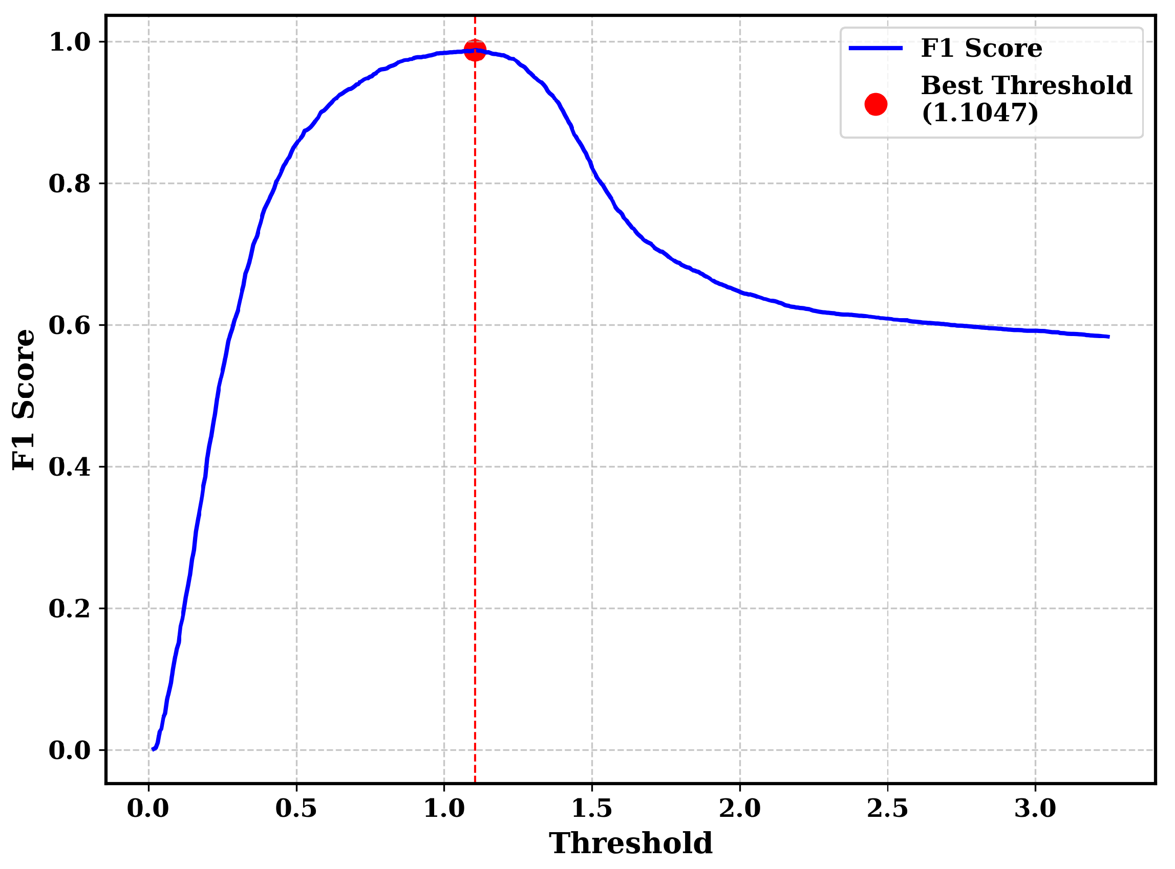
To determine the threshold value to distinguish between known and unknown devices, we used the steps shown in Figure 10 to obtain the f1-score vs. threshold curve, as shown in Figure 12. In this process, the validation sets comprise 10% data from each of the known devices, i.e., devices 1–2 and 5–9, and all the data from device 10. Altogether, the validation set consists of 3386 data frames with 720 I/Q samples in each frame (n = 10, i.e., combining 10 frames to make a single frame). The f1-score [46] combines precision and recall as follows:

$$\mathrm{F}1\text{-}\mathrm{score}=2\times {\displaystyle \frac{\mathrm{Precision}\times \mathrm{Recall}}{\mathrm{Precision}+\mathrm{Recall}}}$$

(10)

where precision is the ratio of true positive predictions to the total positive predictions.

$$\mathrm{Precision}={\displaystyle \frac{\mathrm{TP}}{\mathrm{TP}+\mathrm{FP}}}$$

(11)

and recall (or sensitivity) is the ratio of true positive predictions to the actual positives

$$\mathrm{Recall}={\displaystyle \frac{\mathrm{TP}}{\mathrm{TP}+\mathrm{FN}}}$$

(12)

The f1-score vs. threshold curve is obtained by plotting f1-score values for 500 different values of threshold, ranging from 0 to 3.3. The optimum threshold is the threshold for which we obtain the maximum value of the f1-score. We obtained the optimum threshold of 1.1047, indicated by the red vertical line in Figure 12.

Figure 13 illustrates the scatterplot of the MSSs of the known and unknown devices with SBEC for the validation set. Blue dots represent the MSSs of known devices, and red dots represent those of unknown devices. The horizontal line in the middle indicates the optimum threshold, i.e., 1.1047, for device identification. We can observe a clear distinction between the similarity scores of the known and unknown devices.

5.3. Performance of SBEC

The performance of SBEC in the trained Siamese network is tested in a test set that includes 20% of data from each of seven in-library devices and data from out-of-library devices, which we call “outliers”. The test set consists of a total of 6774 frames with 720 I/Q samples in each frame (n = 10, i.e., combining 10 frames to make a single frame).

5.3.1. Classification Dynamics with Confusion Matrices

The confusion matrix shown in Figure 14 shows the performance of SBEC in classifying in-library devices and out-of-library devices. Strong diagonal dominance is evident, demonstrating that SBEC accurately classifies devices. However, we can observe some misclassification. For example, out of 3984 samples from outlier devices, SBEC correctly detected 3922 (approx. 98.4%) samples. Similarly, SBEC misclassified twelve samples from device 1, seventeen samples from device 2, seven samples from device 5, eleven samples from device 6, and three samples from each of devices 7, 8, and 9 as outliers. No known device was misclassified as another known device; however, some unknown devices were classified as known, and some known devices were classified as unknown. Despite some misclassification, SBEC demonstrates strong performance in classifying known devices and detecting out-of-library devices, achieving an overall accuracy of 98.25%.

5.3.2. Comparison of Precision, Recall, F1-Score, and Accuracy of Each Class

The precision, recall, f1-score, and accuracy of using SBEC to identify in-library and out-of-library devices are shown in Figure 15. All performance metrics, precision, recall, f1-score, and accuracy, remain consistently high across devices, reflecting robust classification. Notably, the unknown class also demonstrates strong detection capability. Device 2 shows slightly lower precision, indicating room for improvement or deeper analysis.

5.4. Tuning Values of Margin (m) and Numbers of Frames Combined (n)

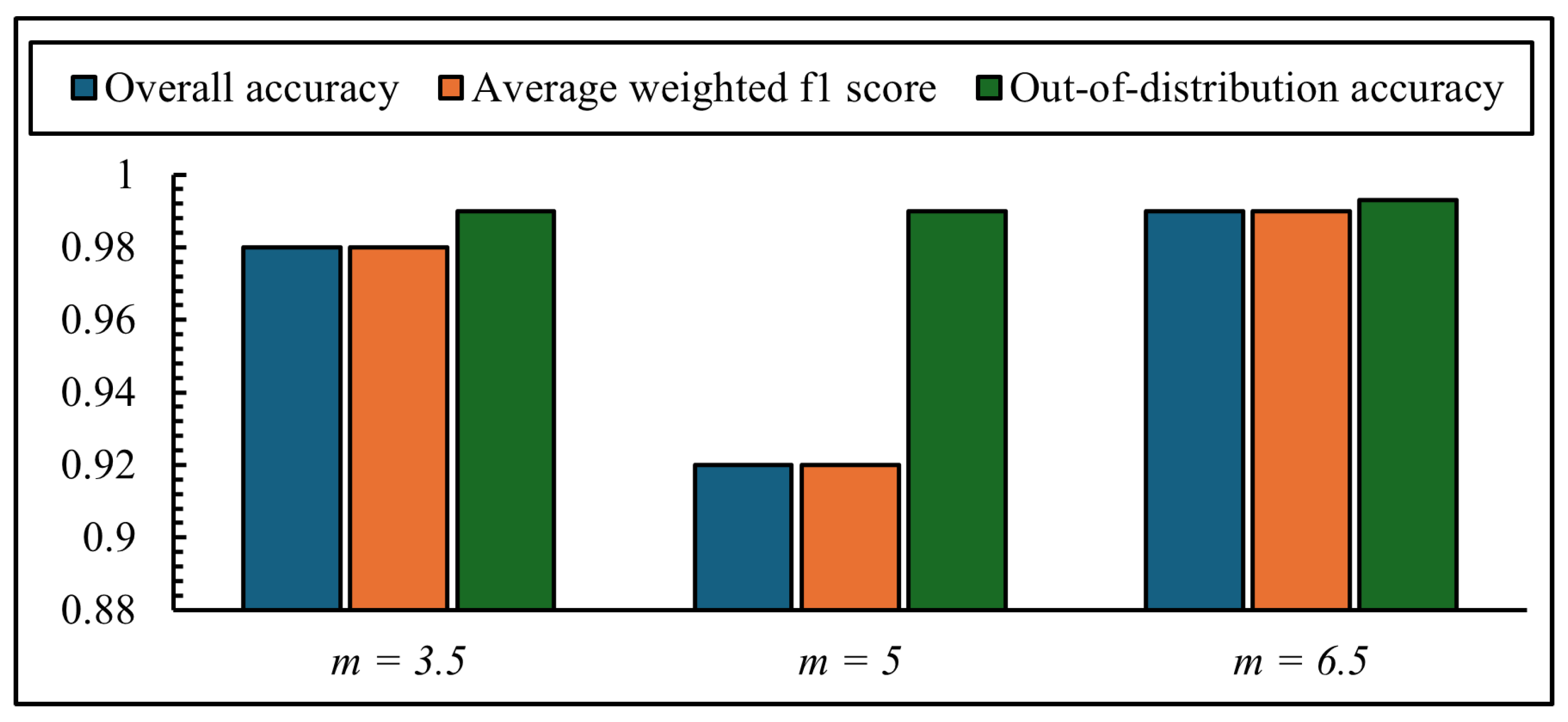
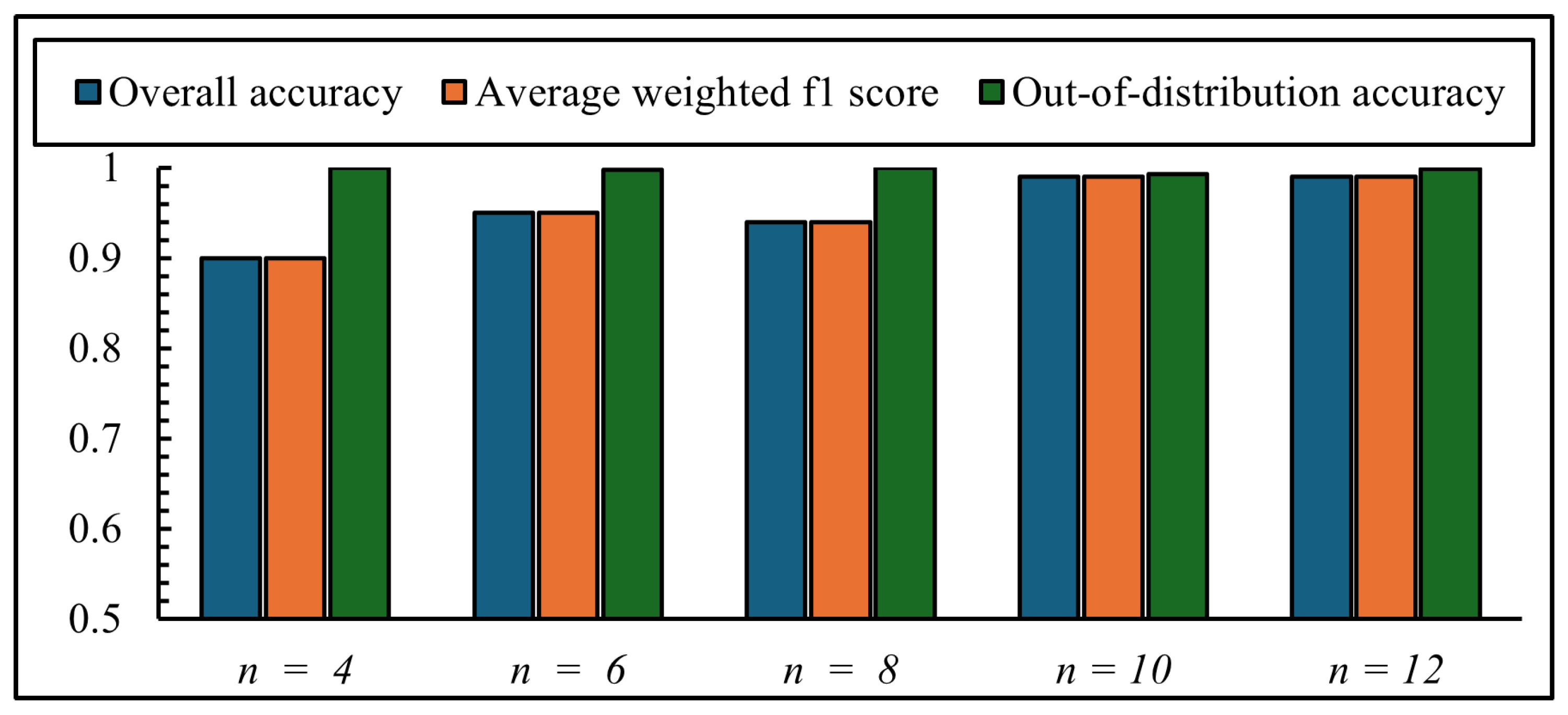
We repeated the experiments by using different values of margin m from 3.5 to 6.5 and the number of frames combined n from 4 to 12. Figure 16 demonstrates the performance of the proposed approach for different values of m. It can be identified that the best performance can be achieved when the value of m is 6.5. Also, Figure 17 shows the performance of the proposed approach for different values of the number of frames combined. It can be inferred from the results of tuning that increasing the value of n improves performance. Based on these results, we selected $m=6.5$ and $n=10$ as the optimal hyperparameters for our final model configuration.

5.5. Performance with Each Device as Unknown

To further test the effectiveness of SBEC, we treated each device as an unknown, one at a time, and checked their performance. Since showing all possible combinations of seven known and two unknown devices is not practical, we focused on key examples to highlight the method’s effectiveness.

Table 2. Performance when considering each device as unknown.

Out-of-Distribution Devices	Overall Accuracy (%)	Average Weighted f1-Score	Out-of-Distribution Accuracy (%)
Device 1	93.60	0.94	96.80
Device 2	95.73	0.96	90.30
Device 3	99.33	0.99	99.00
Device 4	97.72	0.98	100.00
Device 5	96.12	0.96	100.00
Device 6	98.76	0.99	100.00
Device 7	98.32	0.98	100.00
Device 8	98.76	0.99	100.00
Device 9	89.76	0.90	100.00
Device 10	92.80	0.92	91.00

shows the result of the SBEC algorithm when tested, making each of the devices an unknown device. Out-of-distribution accuracy refers to the accuracy in detecting unknown devices, and overall accuracy means the overall accuracy in detecting unknown and classifying known devices. We can observe that the overall performance in the case of devices 3, 4, 5, 6, 7, and 8, as outlier devices, is near perfect. In the case of devices 2, 9, and 10, accuracy remains high (more than 89%), but there is still room for improvement. Even though the model parameters are tuned for devices 3 and 4 as outliers, it works well for other devices as outliers. These findings demonstrate SBEC’s effectiveness in distinguishing unknown devices while maintaining strong overall classification performance.

5.6. Comparison with Existing RF Fingerprinting Methods

To evaluate the effectiveness of the proposed Siamese network model for RF fingerprinting, we compare it with existing methods based on overall accuracy and out-of-library detection capability.

Table 3. Comparison of RF fingerprinting methods, emphasizing out-of-library detection.

Study	Model/Method	Devices	Overall Accuracy (%)	Out-of-Distribution Accuracy (%)	Remarks
Huang et al. [40]	2D-CNN, 2D-CNN combined with bidirectional LSTM, and 3D-CNN	5 ADALM-PLUTO	97.6	N/A	No mechanism for rogue detection.
G. Sun et al. [38]	Combined Siamese networks	12 radios	87	87	Requires the N numbers of Siamese networks for N known devices.
Birnbarch et al. [41]	Siamese network	ADSB/RS485	N/A	81	Limited to differentiating legitimate and adversarial samples.
Roy et al. [47]	GAN, CNN, DNN, RNN	8 USRP B210	97.85 (classification excluding rogue)	99.99	Synthetic samples are considered as rogue.
This work (Proposed)	Siamese network	10 ADALM-PLUTO SDR	98.25	98.4	Learns pairwise similarity; scalable and effective for unseen device detection.

shows the summarized results.

Huang et al. [40] proposed wireless and wired device authentication using density trace plots obtained from constellation, eye, and phase trajectories. They utilized three different deep learning models: 2D-CNN, the combination of 2D-CNN and Long Short-Term Memory (LSTM), and 3D-CNN, achieving an accuracy of 96.7% using signals collected from five different ADALM-PLUTO devices. However, their work was solely focused on identifying known devices, and they did not propose any methods to detect unknown devices. G. Sun et al. [38] proposed to use combined Siamese networks to identify eight known devices and three unknown devices. Their approach achieved an accuracy of 87% by employing multiple Siamese networks, equal to the total number of known devices in the system. In contrast, our method achieved an improved accuracy of 98% while using only a single Siamese network with 5,546,728 parameters (approximately 21.16 MB), regardless of the number of known or unknown devices. For a system with seven known devices, their model requires seven Siamese networks, resulting in a total of $7\times \mathrm{3,113,672}=\mathrm{21,795,704}$ parameters (approximately $7\times 11.88=83.16$ MB). Our model is more efficient as it maintains a single model irrespective of the number of known and unknown devices, while their approach scales linearly with the number of known devices. Additionally, they did not verify the robustness of the approach by repeating the experiments, considering different devices as unknown. In contrast, we repeated the experiment 10 times, treating each device as unknown, and demonstrated the robustness of our work. Additionally, the model in [38] lacks scalability, necessitating retraining from scratch whenever new devices are added to the system as known devices. Birnbarch et al. [41] proposed an adaptable RF fingerprinting system using a Siamese network architecture for both wireless (ADS-B) and wired (RS-485) communication links. Their approach was primarily designed to distinguish between legitimate and adversarial (spoofed) transmissions under targeted attack scenarios. However, their method is limited to differentiating legitimate and adverse samples rather than performing generalized unknown device detection. Their work did not report a standard out-of-library detection accuracy metric; instead, spoofing success rates were used to evaluate performance, with a maximum attacker success rate of 19%, implying an approximate out-of-library detection rate of up to 81% in the worst case. However, this work cannot identify legitimate devices.

The Radio Frequency Adversarial Learning (RFAL) framework proposed by Roy et al. [47] presents the idea of generating synthetic samples using a GAN and exploiting the discriminator part of the trained GAN to differentiate between rogue devices and genuine devices. They verified the proposed system by using I/Q samples collected from eight different USRP B210 SDRs. They obtained an out-of-distribution accuracy of 99.99%. Furthermore, to classify the known devices, they trained three different deep learning models, namely CNN, Dense Neural Network (DNN), and Recurrent Neural Network (RNN), and achieved an accuracy of 97.85% in identifying known devices. Although they achieved higher accuracy in detecting unknown devices and identifying known ones, their test set does not comprise any samples from real devices, meaning that only synthetically generated samples are considered rogue or unknown. Additionally, they need to retrain the model from scratch whenever new devices are added to the environment as legitimate devices.

5.7. Model Complexity and Deployment Within IoT Security Architectures

The Siamese network used in this work consists of 5,546,728 parameters, which hold a memory size of approximately 21.1 MB. The model was trained by using a T4 GPU on Google Colab (High-RAM instance), with a total training time of 2407 s across 100 epochs. The inference behavior of the model after training is highly efficient, with a total inference time of 0.8907 s and an average inference time per sample of 0.000131 s. This rapid execution demonstrates the model’s capability for use in real-time applications. The fast inference time and compact size of the model make it highly suitable for deployment in IoT environments. The 21.1 MB size of the model aligns well with the computational capacity of modern edge devices, such as the Raspberry Pi, Jetson Nano, and AI-enabled microcontrollers. Once the model is trained on high-end devices, such as GPUs, it can be utilized by edge devices in IoT systems to authenticate wireless IoT devices based on their radio frequency fingerprints. Thus, the system enables lightweight and efficient device authentication without requiring extensive computational resources at the edge devices.

The proposed RFF approach, utilizing a Siamese network, can be integrated into existing IoT security frameworks to enhance device authentication at the physical layer. Traditional security approaches for IoT systems often include cryptographic methods such as pre-shared keys, digital certificates, or centralized authentication servers [48,49], which can be difficult to manage and scale, especially in large and heterogeneous networks. On the other hand, our RFF-based approach offers a lightweight and hardware-dependent alternative for authenticating devices based on RF characteristics, thereby eliminating the need for additional overhead or key management. Additionally, this approach can serve as a complementary layer to existing security protocols, thereby providing multi-level authentication that enhances resilience against spoofing and impersonation attacks.

6. Limitations and Future Works

Although promising results are observed, this work has certain limitations that can be addressed in future work. The experimental setup during data collection, when transmitting and receiving signals between stationary ADALM-PLUTO SDR devices, does not account for scenarios where devices are moving, operating in non-line-of-sight conditions, or experiencing a more complicated interference pattern, including multi-path interference, which can affect the performance of the Siamese network. Future research will incorporate data collection in mobile environments, at varying distances, as well as in non-line-of-sight conditions to examine the adaptability and robustness of the proposed algorithms [50]. Additionally, future research shall utilize adaptive signal processing techniques to mitigate the effects of Doppler shifts in the mobile environment [19]. Also, the current approach does not account for temporal variations such as device drift or changes in channel conditions over time. Thus, future work shall aim to incorporate long-term data collection and adaptive training methods to improve robustness against both device drift and dynamic channel environments [19,41]. The Siamese network-based RFF model is susceptible to adversarial attacks, where attackers may not always be rogue devices but could mimic genuine devices by generating signals similar to the original ones. To counter this, future research shall investigate training GANs to generate synthetic samples that closely resemble genuine signals, thereby making it more difficult for adversaries to bypass the system [47]. Furthermore, this work is confined to using data from ten SDRs (considering seven in-library and two out-of-library). However, real IoT environments can have vast numbers of devices. To prove the scalability of the proposed work, future research will expand the number of devices [17]. Additionally, future work can extend this research to demonstrate the scalability of Siamese networks by utilizing devices as in-library devices without involving them in the training process.

7. Conclusions

The use of RF fingerprinting-based authentication addresses the limitation of traditional cryptographic-based approaches, which are unsuitable in resource-constrained environments. In this work, we proposed using a Siamese network to identify RF fingerprints. The Siamese network is advantageous because it works with small datasets and eliminates the need to retrain the model when new legitimate devices are added to the system. We collected I/Q samples from 10 different ADALM-PLUTO SDRs and made them publicly available to contribute further to advancing the research in this domain. In addition, we developed the SBEC algorithm to detect unknown devices and identified known devices and verified their performance in the trained Siamese network using real-world datasets from SDRs. SBEC worked efficiently in identifying known devices and detecting unknown devices, with a high accuracy of 98%. Our study demonstrates that a Siamese network is an efficient and reliable method for device identification, particularly in resource-constrained environments.

References

1. Anani, W.; Ouda, A.; Hamou, A. A survey of wireless communications for IoT echo-systems. In Proceedings of the 2019 IEEE Canadian Conference of Electrical and Computer Engineering (CCECE), Edmonton, AB, Canada, 5–8 May 2019. [Google Scholar] [CrossRef]
2. Premkumar, M.; Arun, M.; Prathipa, R.; Badri Narayanan, D. Signal Transmission and Reception in Wireless Smart Cities. Mater. Today Proc. 2023, 80, 3837–3840. [Google Scholar]
3. Seçkin, A.Ç.; Ateş, B.; Seçkin, M. Review on Wearable Technology in sports: Concepts, Challenges and opportunities. Appl. Sci. 2023, 13, 10399. [Google Scholar] [CrossRef]
4. Pereira, C.E.; Diedrich, C.; Neumann, P. Communication protocols for automation. In Springer Handbook of Automation; Springer: Berlin/Heidelberg, Germany, 2023; pp. 535–560. [Google Scholar]
5. Bout, E.; Loscri, V.; Gallais, A. How Machine Learning Changes the Nature of Cyberattacks on IoT Networks: A Survey. IEEE Commun. Surv. Tutorials 2022, 24, 248–279. [Google Scholar] [CrossRef]
6. Ali, B.S.; Ullah, I.; Al Shloul, T.; Khan, I.A.; Khan, I.; Ghadi, Y.Y.; Abdusalomov, A.; Nasimov, R.; Ouahada, K.; Hamam, H. ICS-IDS: Application of big data analysis in AI-based intrusion detection systems to identify cyberattacks in ICS networks. J. Supercomput. 2024, 80, 7876–7905. [Google Scholar] [CrossRef]
7. Bhat, M.I.; Giri, K.J. Impact of computational power on cryptography. In Multimedia Security: Algorithm Development, Analysis and Applications; Springer: Singapore, 2021; pp. 45–88. [Google Scholar]
8. Zhang, J.; Shen, G.; Saad, W.; Chowdhury, K. Radio frequency fingerprint identification for device authentication in the internet of things. IEEE Commun. Mag. 2023, 61, 110–115. [Google Scholar] [CrossRef]
9. Abbas, S.; Abu Talib, M.; Nasir, Q.; Idhis, S.; Alaboudi, M.; Mohamed, A. Radio frequency fingerprinting techniques for device identification: A survey. Int. J. Inf. Secur. 2024, 23, 1389–1427. [Google Scholar] [CrossRef]
10. Chatterjee, B.; Das, D.; Maity, S.; Sen, S. RF-PUF: Enhancing IoT security through authentication of wireless nodes using in-situ machine learning. IEEE Internet Things J. 2018, 6, 388–398. [Google Scholar] [CrossRef]
11. Ezuma, M.; Erden, F.; Anjinappa, C.K.; Ozdemir, O.; Guvenc, I. Micro-UAV Detection and Classification from RF Fingerprints Using Machine Learning Techniques. In Proceedings of the 2019 IEEE Aerospace Conference, Big Sky, MT, USA, 2–9 March 2019. [Google Scholar] [CrossRef]
12. Jagannath, A.; Jagannath, J.; Kumar, P.S.P.V. A comprehensive survey on radio frequency (RF) fingerprinting: Traditional approaches, deep learning, and open challenges. Comput. Netw. 2022, 219, 109455. [Google Scholar] [CrossRef]
13. Guo, G.; Wang, H.; Bell, D.; Bi, Y.; Greer, K. KNN model-based approach in classification. In Proceedings of the On The Move to Meaningful Internet Systems 2003: CoopIS, DOA, and ODBASE: OTM Confederated International Conferences, CoopIS, DOA, and ODBASE 2003, Catania, Sicily, Italy, 3–7 November 2003; pp. 986–996. [Google Scholar]
14. Vishwanathan, S.; Narasimha Murty, M. SSVM: A simple SVM algorithm. In Proceedings of the 2002 International Joint Conference on Neural Networks. IJCNN’02 (Cat. No.02CH37290), Honolulu, HI, USA, 12–17 May 2002; Volume 3, pp. 2393–2398. [Google Scholar] [CrossRef]
15. Li, Z.; Liu, F.; Yang, W.; Peng, S.; Zhou, J. A Survey of Convolutional Neural Networks: Analysis, Applications, and Prospects. IEEE Trans. Neural Netw. Learn. Syst. 2022, 33, 6999–7019. [Google Scholar] [CrossRef] [PubMed]
16. Kandel, L.N.; Zhang, Z.; Yu, S. Exploiting CSI-MIMO for Accurate and Efficient Device Identification. In Proceedings of the 2019 IEEE Global Communications Conference (GLOBECOM), Waikoloa, HI, USA, 9–13 December 2019; pp. 1–6. [Google Scholar] [CrossRef]
17. Jian, T.; Rendon, B.C.; Ojuba, E.; Soltani, N.; Wang, Z.; Sankhe, K.; Gritsenko, A.; Dy, J.; Chowdhury, K.; Ioannidis, S. Deep learning for RF fingerprinting: A massive experimental study. IEEE Internet Things Mag. 2020, 3, 50–57. [Google Scholar] [CrossRef]
18. Zhao, C.; Yu, J.; Luo, G.; Wu, Z. Radio Frequency Fingerprinting Identification of Few-Shot Wireless Signals Based on Deep Metric Learning. Wirel. Commun. Mob. Comput. 2023, 2023, 2132148. [Google Scholar] [CrossRef]
19. Soltani, N.; Reus-Muns, G.; Salehi, B.; Dy, J.; Ioannidis, S.; Chowdhury, K. RF Fingerprinting Unmanned Aerial Vehicles with Non-Standard Transmitter Waveforms. IEEE Trans. Veh. Technol. 2020, 69, 15518–15531. [Google Scholar] [CrossRef]
20. Cai, Z.; Wang, Y.; Gui, G.; Sha, J. Toward Robust Radio Frequency Fingerprint Identification via Adaptive Semantic Augmentation. IEEE Trans. Inf. Forensics Secur. 2025, 20, 1037–1048. [Google Scholar] [CrossRef]
21. Al-Shawabka, A.; Pietraski, P.; Pattar, S.B.; Restuccia, F.; Melodia, T. DeepLoRa: Fingerprinting LoRa Devices at Scale Through Deep Learning and Data Augmentation. In Proceedings of the MobiHoc ’21, Shanghai, China, 26–29 July 2021; pp. 251–260. [Google Scholar] [CrossRef]
22. Gu, J.; Soltani, N.; Naderi, M.Y.; Chowdhury, K.R. It’s a Bird, It’s a Plane, It’s “That” UAV: RF Fingerprinting During Flight. In Proceedings of the 2021 55th Asilomar Conference on Signals, Systems, and Computers, Pacific Grove, CA, USA, 31 October–3 November 2021; pp. 300–304. [Google Scholar] [CrossRef]
23. Tian, Q.; Lin, Y.; Guo, X.; Wang, J.; AlFarraj, O.; Tolba, A. An Identity Authentication Method of a MIoT Device Based on Radio Frequency (RF) Fingerprint Technology. Sensors 2020, 20, 1213. [Google Scholar] [CrossRef]
24. Chicco, D. Siamese neural networks: An overview. In Artificial Neural Networks; Humana: New York, NY, USA, 2021; pp. 73–94. [Google Scholar]
25. Wang, S.; Peng, L.; Fu, H.; Hu, A.; Zhou, X. A convolutional neural network-based RF fingerprinting identification scheme for mobile phones. In Proceedings of the IEEE INFOCOM 2020-IEEE Conference on Computer Communications Workshops (INFOCOM WKSHPS), Toronto, ON, Canada, 6–9 July 2020; pp. 115–120. [Google Scholar]
26. Shen, G.; Zhang, J.; Marshall, A.; Peng, L.; Wang, X. Radio frequency fingerprint identification for LoRa using deep learning. IEEE J. Sel. Areas Commun. 2021, 39, 2604–2616. [Google Scholar] [CrossRef]
27. Huang, D.; Al-Hourani, A.; Sithamparanathan, K.; Rowe, W.S.; Bulot, L.; Thompson, A. Deep learning methods for device authentication using RF fingerprinting. In Proceedings of the 2021 15th International Conference on Signal Processing and Communication Systems (ICSPCS), Sydney, Australia, 13–15 December 2021. [Google Scholar] [CrossRef]
28. Yu, J.; Hu, A.; Li, G.; Peng, L. A multi-sampling convolutional neural network-based RF fingerprinting approach for low-power devices. In Proceedings of the IEEE INFOCOM 2019-IEEE Conference on Computer Communications Workshops (INFOCOM WKSHPS), Paris, France, 29 April–2 May 2019. [Google Scholar] [CrossRef]
29. Yang, J.; Gu, H.; Hu, C.; Zhang, X.; Gui, G.; Gacanin, H. Deep complex-valued convolutional neural network for drone recognition based on RF fingerprinting. Drones 2022, 6, 374. [Google Scholar] [CrossRef]
30. Li, B.; Cetin, E. Design and evaluation of a graphical deep learning approach for RF fingerprinting. IEEE Sens. J. 2021, 21, 19462–19468. [Google Scholar] [CrossRef]
31. Lee, W.; Baek, S.Y.; Kim, S.H. Deep-learning-aided RF fingerprinting for NFC security. IEEE Commun. Mag. 2021, 59, 96–101. [Google Scholar] [CrossRef]
32. Jafari, H.; Omotere, O.; Adesina, D.; Wu, H.H.; Qian, L. IoT devices fingerprinting using deep learning. In Proceedings of the MILCOM 2018-2018 IEEE Military Communications Conference (MILCOM), Los Angeles, CA, USA, 29–31 October 2018. [Google Scholar] [CrossRef]
33. Otto, A.; Rananga, S.; Masonta, M. Deep Learning vs. Traditional Learning for Radio Frequency Fingerprinting. In Proceedings of the 2024 IST-Africa Conference (IST-Africa), Dublin, Ireland, 20–24 May 2024. [Google Scholar] [CrossRef]
34. Morge-Rollet, L.; Le Roy, F.; Le Jeune, D.; Gautier, R. Siamese network on I/Q signal for RF fingerprinting. In Proceedings of the Conference on Artificial Intelligence for Defense (CAID) 2020, Rennes, France, 26–28 August 2020. [Google Scholar]
35. Alhoraibi, L.; Alghazzawi, D.; Alhebshi, R.; Rabie, O.B.J. Physical layer authentication in wireless networks-based machine learning approaches. Sensors 2023, 23, 1814. [Google Scholar] [CrossRef]
36. Langford, Z.; Eisenbeiser, L.; Vondal, M. Robust Signal Classification Using Siamese Networks. In Proceedings of the WiseML 2019: Proceedings of the ACM Workshop on Wireless Security and Machine Learnin, Miami, FL, USA, 15–17 May 2019. [Google Scholar] [CrossRef]
37. Meng, Q.; Li, G.; Shi, J.; Hu, A. Enhancing RF Fingerprinting with a Simulated Attack Detection Strategy for Few Labeled Signals. In Proceedings of the 2023 IEEE 23rd International Conference on Communication Technology (ICCT), Wuxi, China, 20–22 October 2023; pp. 281–285. [Google Scholar] [CrossRef]
38. Sun, G. RF Transmitter Identification Using Combined Siamese Networks. IEEE Trans. Instrum. Meas. 2022, 71, 1–13. [Google Scholar] [CrossRef]
39. Sankhe, K.; Belgiovine, M.; Zhou, F.; Angioloni, L.; Restuccia, F.; D’Oro, S.; Melodia, T.; Ioannidis, S.; Chowdhury, K. No radio left behind: Radio fingerprinting through deep learning of physical-layer hardware impairments. IEEE Trans. Cogn. Commun. Netw. 2019, 6, 165–178. [Google Scholar] [CrossRef]
40. Huang, D.; Al-Hourani, A.; Sithamparanathan, K.; Rowe, W.S.T. Deep Learning Methods for IoT Device Authentication Using Symbols Density Trace Plot. IEEE Internet Things J. 2024, 11, 18167–18179. [Google Scholar] [CrossRef]
41. Birnbach, S.; Smailes, J.; Baker, R.; Martinovic, I. Adaptable Hardware Fingerprinting for Radio Data Links and Avionics Buses in Adversarial Settings. In Proceedings of the 2023 IEEE/AIAA 42nd Digital Avionics Systems Conference (DASC), Barcelona, Spain, 1–5 October 2023. [Google Scholar] [CrossRef]
42. Nixon, M.S.; Aguado, A.S. 12 - Distance, classification and learning. In Feature Extraction and Image Processing for Computer Vision, 4th ed.; Nixon, M.S., Aguado, A.S., Eds.; Academic Press: Cambridge, MA, USA, 2020; pp. 571–604. [Google Scholar] [CrossRef]
43. Hadsell, R.; Chopra, S.; LeCun, Y. Dimensionality reduction by learning an invariant mapping. In Proceedings of the 2006 IEEE Computer Society Conference on Computer Vision and Pattern Recognition (CVPR’06), New York, NY, USA, 17–22 June 2006; Volume 2, pp. 1735–1742. [Google Scholar]
44. Dhakal, R.; Devkota, B.P.; Niure Kandel, L. Radio Frequency Fingerprinting with Siamese Network. In Proceedings of the 2025 International Conference on Computing, Networking and Communications (ICNC), Honolulu, HI, USA, 17–20 February 2025; pp. 212–216. [Google Scholar] [CrossRef]
45. Jiang, R.; Hu, J.; Huang, H.; Zhang, C.; Wang, L.; Xu, S. A Generalized Radio Frequency Fingerprint-Based Wireless Device Identification Using Siamese-Based Neural Network. IEEE Sens. J. 2025, 25, 23262–23275. [Google Scholar] [CrossRef]
46. Goutte, C.; Gaussier, E. A Probabilistic Interpretation of Precision, Recall and F-Score, with Implication for Evaluation. In Proceedings of the Advances in Information Retrieval, Santiago de Compostela, Spain, 21–23 March 2005; pp. 345–359. [Google Scholar]
47. Roy, D.; Mukherjee, T.; Chatterjee, M.; Blasch, E.; Pasiliao, E. RFAL: Adversarial Learning for RF Transmitter Identification and Classification. IEEE Trans. Cogn. Commun. Netw. 2020, 6, 783–801. [Google Scholar] [CrossRef]
48. Khari, M.; Garg, A.K.; Gandomi, A.H.; Gupta, R.; Patan, R.; Balusamy, B. Securing Data in Internet of Things (IoT) Using Cryptography and Steganography Techniques. IEEE Trans. Syst. Man Cybern. Syst. 2020, 50, 73–80. [Google Scholar] [CrossRef]
49. Mustafa, G.; Ashraf, R.; Mirza, M.A.; Jamil, A.; Muhammad. A review of data security and cryptographic techniques in IoT based devices. In Proceedings of the ICFNDS ’18, Amman, Jordan, 26–27 June 2018. [Google Scholar] [CrossRef]
50. Guo, X.; Zhang, Z.; Chang, J. Survey of Mobile Device Authentication Methods Based on RF Fingerprint. In Proceedings of the IEEE INFOCOM 2019—IEEE Conference on Computer Communications Workshops (INFOCOM WKSHPS), Paris, France, 29 April–2 May 2019. [Google Scholar] [CrossRef]
Figure 1. Transmission and reception of I/Q samples.
Iot 06 00047 g001
Figure 2. Training and testing of Siamese network.
Iot 06 00047 g002
Figure 3. Experimental setup for data collection using ADALM-PLUTO.
Iot 06 00047 g003
Figure 4. Header I/Q samples of one frame from devices 1, 2, and 3.
Iot 06 00047 g004
Figure 5. Payload I/Q samples of one frame from devices 1, 2, and 3.
Iot 06 00047 g005
Figure 6. Probability distribution of in-phase (I) component of header.
Iot 06 00047 g006
Figure 7. Probability distribution of quadrature (Q) component of header.
Iot 06 00047 g007
Figure 8. Convolution layers.
Iot 06 00047 g008
Figure 9. Structure of Siamese network.
Iot 06 00047 g009
Figure 10. Steps to calculate threshold that differentiates between known and unknown devices.
Iot 06 00047 g010
Figure 11. Learning curve of trained Siamese network.
Iot 06 00047 g011
Figure 12. F1-score vs. threshold.
Iot 06 00047 g012
Figure 13. Minimum similarity scores (MSSs) of the data points of known and unknown devices in validation set.
Iot 06 00047 g013
Figure 14. Confusion matrix obtained with SBEC using the test set with known and unknown devices.
Iot 06 00047 g014
Figure 15. Precision, recall, f1-score, and accuracy with SBEC algorithm.
Iot 06 00047 g015
Figure 16. Performance for different values of m.
Iot 06 00047 g016
Figure 17. Performance for different values of n.
Iot 06 00047 g017