Data-Bound Adaptive Federated Learning: FedAdaDB

Abstract

Federated Learning (FL) enables decentralized Machine Learning (ML), focusing on preserving data privacy, but faces a unique set of optimization challenges, such as dealing with non-IID data, communication overhead, and client drift. Adaptive optimizers like AdaGrad, Adam, and Adam variations have been applied in FL, showing good results in convergence speed and accuracy. However, it can be quite challenging to combine good convergence, model generalization, and stability in an FL setup. Data-bound adaptive methods like AdaDB have demonstrated promising results in centralized settings by incorporating dynamic, data-dependent bounds on Learning Rates (LRs). In this paper, FedAdaDB is introduced, which is an FL version of AdaDB aiming to address the aforementioned challenges. FedAdaDB uses the AdaDB optimizer at the server-side to dynamically adjust LR bounds based on the aggregated client updates. Extensive experiments have been conducted comparing FedAdaDB with FedAvg and FedAdam on three different datasets (EMNIST, CIFAR100, and Shakespeare). The results show that FedAdaDB consistently offers better and more robust outcomes, in terms of the measured final validation accuracy across all datasets, for a trade-off of a small delay in the convergence speed at an early stage.

1. Introduction

Obtaining good user data has always been a critical task for Machine Learning (ML) applications. Innovative model architectures like Diffusion models and Transformers are trained on an enormous amount of data to provide satisfying results. Data can be obtained either from well-curated datasets or by crawling the open internet. Furthermore, accessing new end-user data or data collected or generated by Internet of Things (IoT) devices can be beneficial, especially in terms of fine-tuning and personalization. However, there is a vital matter of privacy when handling user data, therefore, Federated Learning (FL) has been proposed as a solution [1], enabling decentralized training across multiple clients while maintaining data privacy. With the FL approach, clients train a shared global model on their local data, with the coordination of a central server. Clients send only the model weight updates, and their raw data are not shared with other clients or the central server. This method can be beneficial, especially in cases where data privacy and security are prioritized, such as in healthcare, finance, and mobile applications [2,3].

FL may offer some important advantages; however, it also presents several distinctive challenges compared to centralized or classic Distributed Machine Learning (DML), particularly in the realm of optimization [4]. The primary obstacles include handling non-independent and identically distributed (non-IID) data across clients, managing communication overhead, and ensuring model convergence despite intermittent partial client participation [5,6,7,8,9]. Classic optimization techniques like Stochastic Gradient Descent (SGD) tend to be more sensitive to hyperparameter selection and tuning; therefore, they often struggle in such environments [10]. Additionally, client data heterogeneity and the decentralized nature of FL tend to worsen troubling issues such as client drift, where local model updates diverge from the global objective, leading to suboptimal performance and slower convergence [11,12].

To overcome these challenges, adaptive optimization methods have gained popularity in FL. These methods dynamically adjust Learning Rates (LRs) based on the historical gradient information, therefore enhancing convergence speed and model generalization [13,14,15]. Adaptive optimizers such as Adam, Yogi, or Adagrad have been proposed as server optimizers in FL settings [10], showing positive findings by tackling issues related to hyperparameter sensitivity and gradient noise. However, convergence speed and generalization are more challenging issues when dealing with non-IID data in an FL setting. Adabound and AdaDB have been proposed as a way to address these challenges, and they demonstrate promising results in centralized and DML training [16,17]. These methods introduced the concept of bound adaptive optimization, an innovative strategy adding an element-wise clipping operation, thus providing faster convergence and better generalization. Traditional adaptive optimizers do not consider the variability in data distribution across clients, which can lead to inefficient updates and slower convergence.

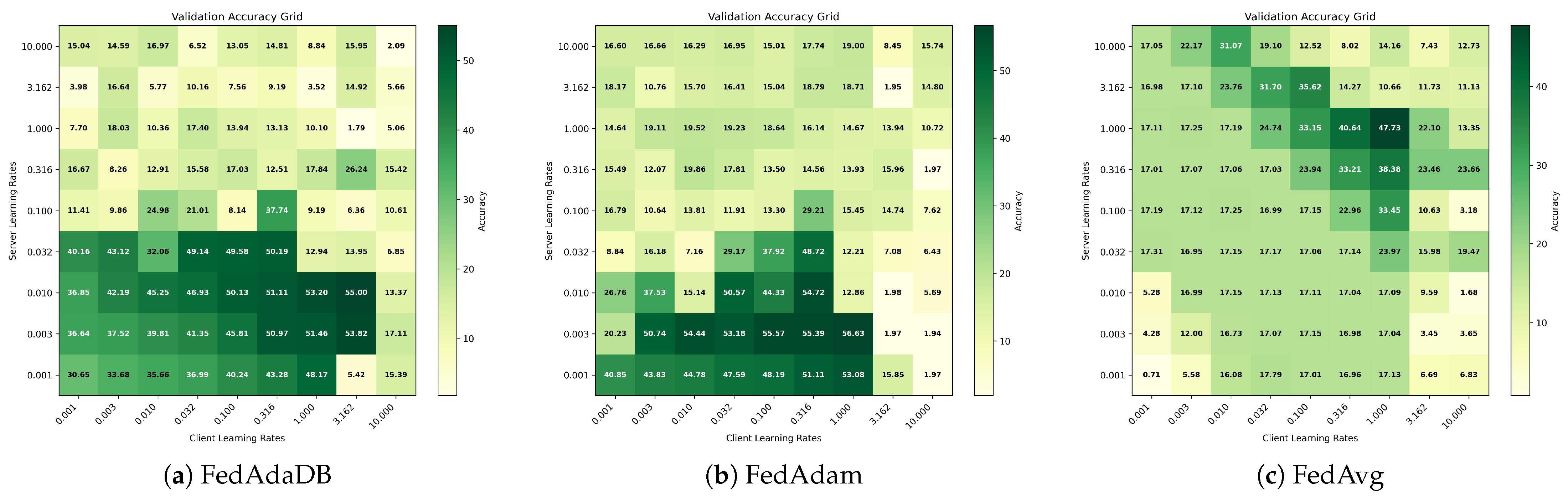
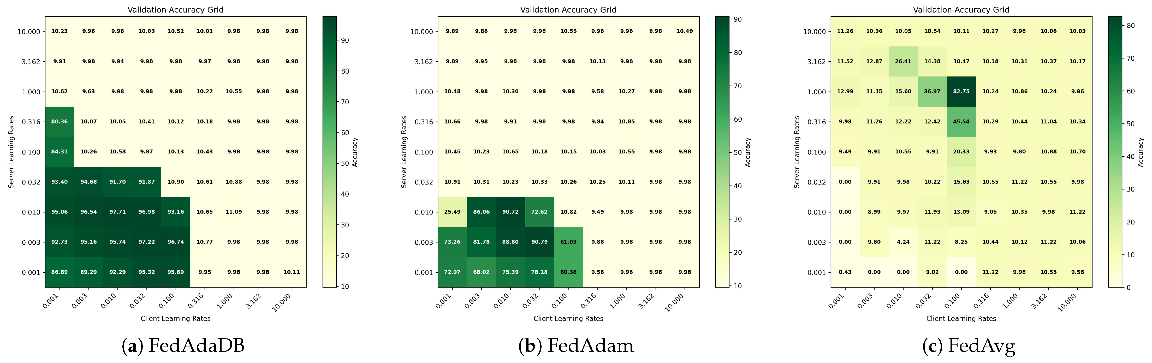
In this research, AdaDB is adapted in the FL setting (FedAdaDB), investigating the power of a data-bound adaptive optimizer in an FL setting. The proposed data-bound adaptive algorithm, FedAdaDB, incorporates data-specific characteristics into the optimization process. By adapting LRs not just based on gradient history but also indirectly based on the nature of the data of each client, this algorithm attempts to achieve faster convergence and more robust performance in the FL context. This paper demonstrates notable advancements in the field of federated optimization through the development and evaluation of FedAdaDB. Some of the paper contributions are as follows: (1) Algorithm Innovation: The introduction of the FedAdaDB algorithm, which leverages data-bound techniques to dynamically adjust optimization strategies based on client-specific data characteristics, improving the efficiency and effectiveness of the learning process. (2) Empirical Validation: Through extensive experiments on diverse FL benchmarks, it is shown that FedAdaDB can improve convergence speed, model accuracy, and robustness to data heterogeneity compared to traditional and existing adaptive federated optimizers. (3) Algorithm comparison: FedAdaDB results are compared with the results of the baseline non-adaptive algorithm FedAvg and the widely used FedAdam adaptive algorithm on three different datasets and learning tasks. The algorithms’ hyperparameters are meticulously fine-tuned via grid search to ensure a balanced comparison of every algorithm’s best performance.

2. Related Work

2.1. Adaptive Optimizers

Adaptive optimizers were developed to overcome the limitations of traditional gradient descent methods like SGD, which use a fixed LR for all parameters throughout training. Selecting a fixed small LR may lead to slow convergence or sticking to a suboptimal local minimum. Similarly, using a fixed large LR can cause overshooting and instability [18,19]. Adaptive optimizers have been suggested as a way to address these issues [20]. Adaptive optimizers adjust the LR dynamically, based on the gradient history. Therefore, they can achieve faster and more stable convergence, especially when dealing with sparse or noisy data. Adaptive Gradient Algorithm (AdaGrad) is an adaptive algorithm that adapts the LR based on the historical gradients accumulated during training [21]. This approach provides larger updates for infrequent features and smaller updates for frequent ones. Accumulating all past squared gradients in the AdaGrad denominator may force the LR to monotonically decrease over time. This behavior could cause the training process to slow down at an early stage or even stop, especially when dealing with non-convex optimization landscapes. RMSProp was proposed as a solution to the aforementioned issue [22]. RMSProp modifies AdaGrad’s approach by utilizing a moving average of squared gradients to normalize the gradient, instead of using the entire history. By taking only recent gradient information into consideration, RMSProp maintains higher LRs when needed, helping to avoid premature convergence. A significant leap forward for adaptive optimizers came with the introduction of Adaptive Moment Estimation (Adam) [23]. Adam combined the advantages of AdaGrad and RMSProp, maintaining running averages of both the gradients and their squared values. This approach provides an adaptive LR that converges faster and generalizes better [24]. As Adam gained widespread adoption, many variants have been proposed to improve Adam’s performance in different scenarios. Notable extensions include AdaMax, which uses the infinity norm for parameter updates, and Nadam, which integrates Nesterov momentum into Adam [25]. Yogi was proposed as an alternative to Adam, designed to better control the update magnitude, especially in noisy environments [26] and, therefore, achieve better stability and convergence. More recently, AdaScale was presented, focusing on the challenges of large-batch training scenarios [27]. AdaScale adjusts the LR based on the effective batch size, maintaining the benefits of adaptive methods in large-scale training.

2.2. Optimizers with Learning Rate Bound

AdaBound uses a similar adaptive LR like Adam, but it alternates it by introducing dynamic lower and upper bounds that tighten as training progresses [16,28,29]. Initially, these bounds are broad, enabling rapid learning similar to Adam. As the training rounds pass, the bounds shrink gradually, making the LR more stable and similar to SGD. This transition prevents overly aggressive updates that can occur with adaptive methods, while offering better generalization by eventually adopting the stable LR behavior of SGD. AdaDB further extended the previous idea [17]. AdaDB introduces a novel approach by implementing data-dependent bounds. It utilizes normalized momentum information to create individualized upper and lower bounds for each parameter’s LR. This approach allows AdaDB to be more responsive to the specific characteristics of the data and gradient information. Like AdaBound, it gradually converges to SGD-like behavior but does so in a way that is more aligned to the actual data. This data-dependent strategy potentially leads to better generalization and stability across various training scenarios, although it might present a slight decrease in convergence speed compared to AdaBound.

2.3. Federated Adaptive Optimization

The first FL algorithms, like FedAvg, used an SGD for both server-side and client-side optimizers [1]. However, similarly to centralized learning, FL can also benefit from the use of adaptive optimizers. Therefore, researchers introduced a set of federated adaptive optimizers that extend traditional adaptive methods to the FL setup [10]. These include FedAdam, FedYogi, and FedAdaGrad, each optimized to handle the complexities of federated environments. FedAdam incorporates server-side adaptive updates to manage non-IID data. FedYogi adapts the Yogi optimizer, benefiting from its stability and robustness to noisy gradients in an FL context. And FedAdaGrad extends the AdaGrad algorithm, maintaining adaptive LRs across devices to effectively manage local data distributions. Theoretical and empirical analyses have shown significant improvements in terms of convergence and robustness, despite the inherent heterogeneity in federated data. Another study proposed FedUR [30]. Rather than directly extending centralized methods, the authors analyze the convergence upper bounds associated with both local iterations and global aggregations. By carefully tuning the momentum and adaptive LR parameters, FedUR minimizes the non-vanishing solution bias introduced by multiple local updates. Experimental results confirm that FedUR enhances convergence accuracy while also lowering communication overhead. Another adaptive optimizer in the FL setup is AdaBest [31], a novel reduced-variance local SGD method that counters client drift by adaptively estimating and correcting the bias in local updates. This approach introduces a stabilizing factor that not only mitigates the explosive growth seen in previous methods but also generalizes FedAvg by dynamically adapting to changes in client participation. This results in both faster convergence and improved performance. FedLion is another adaptive FL algorithm that is based on the centralized Lion optimizer [13]. By employing sign-based gradient updates, FedLion reduces the communication payload while achieving a significantly accelerated convergence rate compared to traditional FedAvg. A novel approach was presented with the introduction of FedCAda [32], which enhances FL by applying an Adam-like adaptive optimization directly on the client-side. By carefully constraining the adaptive parameters, especially in the early training stages, the algorithm achieves both rapid convergence and improved stability under non-IID conditions. This method addresses instability and excessive communication overhead by reducing the need to transmit multiple full-precision vectors. Another suggestion for client-side adaptive optimization was introduced in [33], where the authors proposed FAFED, an FL algorithm that uses a shared adaptive learning rate across all clients during their local updates to achieve faster and more stable convergence.

3. Data-Bound Adaptive Federated Learning

In this section, the basic FL problem is formulated, and the role of the FedAdaDB optimizer in addressing this optimization problem is discussed. The notations used throughout the paper are introduced, and the algorithmic steps of the data-bound adaptive optimizers in the FL setup are presented and described.

3.1. Federated Learning Problem Formulation

FL deals with an optimization problem of the form

$$\underset{w}{min}f\left(w\right)=\sum _{i=1}^n{F}_i\left(w\right),$$

(1)

where n is the total number of clients and $F_i\left(w\right)$ is the local objective function of the i-th client. For each client $i\in \{1,2,\dots ,n\}$, an unbiased stochastic gradient $g_i\left(w\right)$ of the client’s true gradient $\nabla F_i\left(w\right)$ is assumed. The following assumptions should apply to guarantee convergence: (1) Each $F_i\left(w\right)$ is L-smooth for all $x,y\in {\mathbb{R}}^d$; that is, $\parallel \nabla F_i\left(x\right)-\nabla F_i\left(y\right)\parallel \le L\parallel x-y\parallel$. (2) The function $F_i\left(x\right)$ satisfies $\parallel \nabla F_i\left(x\right)\parallel \le G$ for all $x\in {\mathbb{R}}^d$.

A typical FL training round begins with the server initializing the global model $w\left(0\right)$. Then, in each round t, a subset $S\left(t\right)=\{1,2,\dots ,C\}$ of randomly sampled clients is selected, and each client $c\in S\left(t\right)$ performs local training on its data for E epochs, resulting in a local model $w_c^{(t,E)}$. Local model change is defined as ${\Delta }_c^{\left(t\right)}=w_c^{(t,E)}-w_c^{(t,0)}$. Afterward, each client sends ${\Delta }_c^{\left(t\right)}$ back to the server. The server then aggregates these local changes and updates the global model as

$$w^{(t+1)}=w^{\left(t\right)}+{\displaystyle \frac{{\sum }_{c\in S\left(t\right)}{p}_c{\Delta }_c^{\left(t\right)}}{{\sum }_{c\in S\left(t\right)}{p}_c}},$$

(2)

where $p_c$ is a relative weight for client c. This procedure continues in a loop until the global model converges.

3.2. Overview of Data-Bound Approach

As stated before, FL faces a unique set of challenges compared to centralized or other distributed ML settings. Client data in FL are usually unevenly distributed and are subject to great heterogeneity (non-IID). This characteristic, alongside client hardware limitations and differences, can lead to local models converging to different optima or enhance a phenomenon called client drift, a situation where local models diverge significantly from the global model, rendering global convergence even more challenging [5,7,12,31]. AdaDB attempts to mitigate some of these challenges by incorporating a data-dependent bounded learning rate $\eta$ [17]. AdaDB operates similarly to the Adam optimizer. Therefore, it calculates $m^{\left(t\right)}$, which is the exponential moving averages of the gradient ${\Delta }^{\left(t\right)}$, and the second moment $v^{\left(t\right)}$. Then, $m^{\left(t\right)}$ and $v^{\left(t\right)}$ are bias-corrected by dividing them by the respective decay rates ($1-{\beta }_1^t$ and $1-{\beta }_2^t$). The main difference resides in the update rule for the model parameters $w^{(t+1)}=w^{\left(t\right)}+\eta ·{\widehat{m}}^{\left(t\right)}$. The crucial part of this rule is the effective LR $\eta$, which is calculated element-wise by clipping an LR vector ${\eta }_s/\sqrt{{\widehat{v}}^{\left(t\right)}}$, between a constant lower bound ${\eta }_l$ and a dynamic upper bound ${\eta }_u$.

$$\eta =\mathrm{clip}\left({\eta }_l,{\displaystyle \frac{{\eta }_s}{\sqrt{{\widehat{v}}^{\left(t\right)}}}},{\eta }_u\right),$$

(3)

where:

• ${\eta }_s$ is the initially selected LR,
• ${\widehat{v}}^{\left(t\right)}={\displaystyle \frac{v^{\left(t\right)}}{1-{\beta }_2^t}}$ is the bias corrected second moment calculation:
  $v^{\left(t\right)}={\beta }_2{v}^{(t-1)}+(1-{\beta }_2){\left({\Delta }^{\left(t\right)}\right)}^2$,
• ${\eta }_u=r+{\eta }_f$ is the dynamic upper bound,
• ${\eta }_l={\eta }_f$ is the constant lower bound.

The r term in the upper bound calculation is the normalized momentum ${\widehat{m}}^{\left(t\right)}$ and is defined as:

$$r={\displaystyle \frac{{\widehat{m}}^{\left(t\right)}}{max\left(|{\widehat{m}}^{\left(t\right)}|\right)·ϵ·t}}$$

(4)

Here, $ϵ·t$ is a decay factor, where $ϵ$ is a small constant for numerical stability and t is the current round index.

A key aspect of this upper bound is its dependence on the magnitude of the momentum. A larger momentum for a particular parameter leads to a larger upper bound on its LR, permitting larger step sizes in that direction, and a smaller momentum results in a smaller upper bound, respectively, thus encouraging smaller updates. The lower bound for every element of the LR vector is simply the constant final LR, ${\eta }_f$. As training progresses, the difference between the upper and lower bounds of both parameters will diminish. At this stage, the optimization process resembles standard SGD with a fixed LR. This mechanism highlights AdaDB’s ability to provide a more tailored and responsive learning process for individual parameters compared to optimizers with static or uniformly changing LR constraints.

3.3. Application to Federated Learning

In a typical FL setup, there are usually two types of optimizers that have to be selected: a client-side optimizer and a server-side optimizer. During each communication round, clients perform several steps of the client-side optimizer on their local datasets and subsequently send their updated model parameters or gradients back to a central server. Then, the server aggregates the updates and updates the global model using the server-side optimizer. Although using adaptive optimizers on the client side might seem beneficial for accelerating local training, it presents certain drawbacks in the federated context. A primary concern is the potential increase in communication costs [34]. Adaptive optimizers often maintain additional state variables, such as momentum and variance estimates, which would need to be communicated to the server along with the model updates, potentially increasing the upload communication overhead. Therefore, adaptive optimizers are usually selected as server-side optimizers, while a simple SGD is usually preferred for the client-side [10,30,31]. Accordingly, AdaDB was used as a server-side optimizer in the context of this paper. Since AdaDB dynamically updates the LR bounds based on the clients’ data, it would be intuitively fair to assume that AdaDB would not be fully exploited on the server side. Even though the server in an FL setting does not have direct access to the clients’ raw data, the aggregated weight updates received from the clients provide valuable information about the learning progress. These aggregated updates essentially represent the average direction and magnitude of the SGD performed across all participating clients in that round. While the updates are based on local data distributions, their collective movement reflects the descent tendency of the global objective function. By employing an AdaDB optimizer on the server side, the server can track the model weight changes and the momentum based on the history of the aggregated weights over multiple rounds. Therefore, the central server can infer the overall progress and the general direction of improvement for the global model and accelerate learning in this direction.

3.4. Proposed Algorithm FedAdaDB

AdaDB dynamically adjusts its LR bounds based on the momentum $m^{\left(t\right)}$ of the gradients, making it responsive to the client data being processed. FedAdaDB uses AdaDB as a server-side optimizer. Although the server lacks direct access to individual client gradients, the aggregated updates ${\Delta }^{\left(t\right)}$ maintain useful information about the underlying client data distributions. They provide valuable insights into the learning progress and the characteristics of the global loss function. These aggregated updates essentially represent the average direction and magnitude of the SGD performed across all participating clients. Their collective movement reflects the descent tendency of the global objective function. The vector difference of the global model in successive rounds serves as a strong proxy for collective learning progress and data characteristics. Research substantiates the idea that this aggregated information is a valuable asset. The authors in [35] leverage the aggregated gradient not just as a direction but also as a strategic tool to explore the loss landscape and guide the global model toward more general solutions. Furthermore, the FedBSS method is built on the premise that the global model, which results from aggregation, can be used to infer the quality and characteristics of individual data samples at the client level by measuring their loss against the global model [36]. This explicitly links the aggregated knowledge back to the bias of local samples. The information richness of these aggregates is further underscored by privacy research. Studies show that it is possible for a malicious server to deconstruct aggregated updates to infer the private data of a specific cohort by manipulating the parameters of the distributed model and using predictable differences in client behavior [37]. Additionally, there is a connection between the properties of the loss landscape and model generalization. Solutions that generalize well have been observed to reside in flat minima of the loss landscape, as opposed to sharp minima [38,39]. The work in [35] suggests that, even with non-IID client data, the loss landscapes of individual clients often share similarities, and importantly, the flat optimal regions of different clients are more likely to partially overlap than sharp optimal regions. If the aggregated gradients effectively guide the global model towards these overlapping flat areas, they are, in effect, reflecting a desirable global property that is indirectly shaped by the collective characteristics of the client data landscapes. In the context of FedAdaDB, the momentum of aggregated weight updates is observed as a meaningful, data-informed signal. This momentum, derived from the gradient updates of all participating clients, reflects the dominant trends and data-driven directions in the weight space. By using this signal to dynamically set the bounds of the LR, FedAdaDB effectively implements a server-side, data-dependent optimization strategy, leveraging the implicit information about client data heterogeneity and learning dynamics embedded within the aggregated updates to achieve more stable and robust convergence.

3.4.1. Algorithm Description

The pseudocode of the suggested FedAdaDB algorithm is presented in Algorithm 1.

Algorithm 1: FedAdaDB Psuedocode
	Input: $w_0,v_{-1},{\beta }_1,{\beta }_2\in [0,1),ϵ,{\eta }_s,{\eta }_f,{\eta }_c$
	Output: Global model $w_T$
1	foreach round $t\in \{1,2,\dots ,T\}$  do
2			$S^{\left(t\right)}\leftarrow \{1,2,\dots ,C\}$
3			foreach client $c\in S^{\left(t\right)}$in parallel  do
4					/* Initialize local model on client c		*/
5					$w_c^{(t,0)}\leftarrow w^{\left(t\right)}$
6					foreach epoch $e\in \{1,2,\dots ,E\}$  do
7						/* Compute stochastic gradient on client c	*/
8						$g_c^{(t,e)}\leftarrow \nabla f_c\left(w_c^{(t,e)}\right)$
9						/* Perform local update (SGD) on client c	*/
10						$w_c^{(t,e+1)}\leftarrow SGD\left(w_c^{(t,e)},g_c^{(t,e)},{\eta }_c,t\right)$
11					end
12					/* Compute local model change after E epochs		*/
13					${\Delta }_c^{\left(t\right)}\leftarrow w_c^{(t,E)}-w_c^{(t,0)}$
14			end
15			/* Aggregate local model changes				*/
16			${\displaystyle {\Delta }^{\left(t\right)}\leftarrow \frac{{\sum }_{c\in S^{\left(t\right)}}{p}_c{\Delta }_c^{\left(t\right)}}{{\sum }_{c\in S^{\left(t\right)}}{p}_c}}$
17			/* Update first and second moment estimators				*/
18			$m^{\left(t\right)}\leftarrow {\beta }_1{m}^{(t-1)}+(1-{\beta }_1){\Delta }^{\left(t\right)}$
19			$v^{\left(t\right)}\leftarrow {\beta }_2{v}^{(t-1)}+(1-{\beta }_2){\left({\Delta }^{\left(t\right)}\right)}^2$
20			/* Bias correction				*/
21			${\widehat{m}}^{\left(t\right)}\leftarrow {\displaystyle \frac{m^{\left(t\right)}}{1-{\beta }_1^t}}$
22			${\widehat{v}}^{\left(t\right)}\leftarrow {\displaystyle \frac{v^{\left(t\right)}}{1-{\beta }_2^t}}$
23			/* Compute adaptive learning rate $\eta$ and clipping				*/
24			$r\leftarrow {\displaystyle \frac{{\widehat{m}}^{\left(t\right)}}{max\left(|{\widehat{m}}^{\left(t\right)}|\right)·ϵ·t}}$
25			${\eta }_u\leftarrow r+{\eta }_f$
26			${\eta }_l\leftarrow {\eta }_f$
27			$\eta =\mathrm{clip}\left({\eta }_l,{\displaystyle \frac{{\eta }_s}{\sqrt{{\widehat{v}}^{\left(t\right)}}}},{\eta }_u\right)$
28			/* Update global model				*/
29			$w^{(t+1)}\leftarrow w^{\left(t\right)}+\eta ·{\widehat{m}}^{\left(t\right)}$
30	end
31	return  $w_T$

The $\eta$ vector computed in code line 27 represents the effective LR and is used for the element-wise weight update in code line 29. It is described in more detail on Equation (3).

3.4.2. On the Convergence of FedAdaDB

A formal, extended convergence analysis of FedAdaDB in the FL setting presents unique challenges and is an open task for future work. However, strong parallels can be extended based on AdaDB’s convergence analysis [17]. The experimental results obtained in this study further lend empirical support to FedAdaDB’s stable convergence. The authors of the AdaDB paper establish two conditions under which Adam-like optimizers can converge in a non-convex setting. More specifically, Adam-like optimizers can converge if their effective learning step ${\displaystyle \frac{{\eta }_s}{\sqrt{v^{(}t)}}}$ is bounded by two functions, (${\eta }_l\left(t\right)$ and ${\eta }_u\left(t\right)$), under the following two conditions:

• ${\eta }_l\left(t\right)$ and ${\eta }_u\left(t\right)$ are two limited functions, and for any $t\ge 0$, ${\eta }_l\left(t\right)\le {\eta }_u\left(t\right)$.
• There is a constant integer quantity $M>0$, when $t\ge M$, ${\eta }_u\left(t\right)-{\eta }_l\left(t\right)\le C{\displaystyle \frac{1}{t}}$.

Based on those two conditions, ${\eta }_l\left(t\right)$ and ${\eta }_u\left(t\right)$ have been proven to converge to the constant final learning rate ${\eta }_f$. Furthermore, the AdaDB paper states that AdaDB’s specific construction of its data-dependent bounds adheres to the above conditions. In AdaDB, the lower bound for each element i is equal to the final learning rate (${\eta }_l\left(t\right)={\eta }_f$), and the upper bound is ${\eta }_u\left(t\right)={\eta }_f+r_i/(ϵ·t)$, where $r_i$ is derived from the normalized momentum, such that $0<r_i\le 1$. Thus, ${\eta }_f+r_i\le {\eta }_f+{\displaystyle \frac{1}{ϵ·t}}$. These two functions satisfy the aforementioned conditions; therefore, AdaDB can converge. In FedAdaDB, the AdaDB optimizer is employed at the server level. The core mechanism of AdaDB, namely the data-dependent upper bound (${\eta }_u=r+{\eta }_f$) and the constant lower bound (${\eta }_l={\eta }_f$), exists as in the server-side update rule of FedAdaDB. The term r in FedAdaDB is derived from the aggregated momentum. Since these bounding structures and their adaptive nature based on momentum are directly adopted by FedAdaDB, it is assumed that FedAdaDB can also converge. Although this does not replace a formal proof that models client drift and suffer from partial participation, it does provide a solid rationale for why the core bounding mechanism of AdaDB remains effective in the FL setting, and it is empirically validated by the extended experiments conducted in the current research.

4. Experimental Setup

FedAdaDB was evaluated and compared with other popular FL algorithms, against different datasets and learning tasks. More specifically, FedAdaDB was compared with the baseline non-adaptive algorithm FedAvg and the widespread adaptive FedAdam. In this section, a detailed description of the experimental setup will be presented. The section includes information about the training hardware, the datasets used, the ML models, and the learning tasks. Moreover, there is a subsection dedicated to the algorithms’ hyperparameter tuning procedure. The experiments were conducted on an Nvidia DGX V100 Workstation using a single Tesla V100 DGXS 32GB GPU (supplied by NVIDIA Corporation, Santa Clara, CA, USA). The implementation of all algorithms and models was carried out using the TensorFlow Federated (TFF) framework [40]. All the algorithms were tested against the same ML tasks to ensure a balanced comparison. Additionally, statistical tests were conducted to assure the statistical significance of the results.

4.1. Datasets and Models

For the task of character recognition, a federated version of the EMNIST dataset [41], with 62 classes and 3383 total clients, is used. The training and testing split occurs per example number. Both training and testing datasets have all 3383 clients, but their examples are split, keeping 671,585 examples for training and 77,483 examples for testing, respectively. EMNIST is used to train a Convolutional Neural Network (CNN) model. The CNN consists of two 5 × 5 convolution layers. The first convolution layer has 32 channels, and the second has 64 channels. Each convolution layer is followed by a 2 × 2 max-pooling layer. After the convolutional layers, there is a fully connected layer with 512 units and ReLU activation, and a final softmax output layer. The total number of parameters in the model is 1,690,046.

For the image classification task, a federated version of the CIFAR100 dataset was used [42]. The CIFAR100 dataset consists of 60,000 32 × 32 color images in 100 classes. For the FL setup, the dataset is split into 500 clients for training and 100 clients for testing, with 100 images on each client. CIFAR100 is used to train a CNN model. The CNN model consists of two main convolutional blocks followed by a dense classification head. The first convolutional block begins with two consecutive 3 × 3 convolution layers, both using 32 channels and ReLU activation. This block is followed by a 2 × 2 max-pooling layer and a dropout layer with a rate of 0.25. The second convolutional block mirrors the first, while also increasing the channel depth. It has two 3 × 3 convolution layers, both with 64 channels and ReLU activation. It is also followed by a 2 × 2 max-pooling layer and a dropout layer. After the convolutional blocks, the feature maps are flattened. The classification head consists of a fully connected layer with 512 units and ReLU activation, followed by a dropout layer with a rate of 0.5. The final layer is a dense output layer with 100 units, corresponding to the 100 CIFAR100 classes. The total number of parameters in this model is 2,214,532.

For the Next-Character-Prediction (NCP) task, a federated version of the Shakespeare dataset is used [43]. The Shakespeare dataset consists of 715 total clients. Instead of using different users for training and testing splits, all 715 clients appear in both datasets, but with different examples. Namely, there are 16,068 examples in the training set and 2356 examples in the testing set. The Shakespeare dataset is used to train a Recurrent Neural Network (RNN). This RNN has an input layer that takes variable-length sequences of words. The Embedding layer transforms each token into a 256-dimensional vector. Following this embedding stage, the sequences traverse through a Gated Recurrent Unit (GRU) layer with 1024 units. The GRU layer delivers sequences of equal length, with each step generating a 1024-dimensional vector. Then, there is a dense layer comprising 66 nodes, aligning with the dimensionality of the output vocabulary. The model has a total of 4,022,850 trainable parameters.

Data Distribution on Different Clients

All three federated datasets have non-IID data. In this subsection, an example of the dataset’s unbalanced nature will be presented, by selecting a random sample of 10 clients and analyzing their local data. More specifically, Figure 1, Figure 2 and Figure 3 visualize the following: (a) The Number of Samples for every client. This is the total count of data points (e.g., images for EMNIST and CIFAR100, or characters for Shakespeare). This metric reflects the quantity of data on each client, highlighting imbalances in data contribution. (b) The Number of Classes, or Unique Characters. A measure of label diversity per client. (c) The Normalized Entropy. This uses the Shannon entropy of a client’s local data distribution to quantify the diversity of the client’s data. (d) The Gini Coefficient. It describes how balanced the samples are in each class. (e) The Kullback–Leibler (KL) Divergence. This metric quantifies how different a client’s data distribution is from the average global distribution. (f) The Dominant Class/Character Percentage. The proportion of a client’s local data that belongs to the most frequent class or character.

4.2. Learning Rate Tuning

In FL, there are usually at least two LRs that need to be tuned, the client optimizer’s LR (${\eta }_c$) and the server optimizer’s LR (${\eta }_s$). To make sure that the best client–server LR pair is selected, a grid search was employed [44] on a 9 × 9 grid, with LRs logarithmically spaced between ${10}^{-3}$ and ${10}^1$. Each algorithm was fine-tuned separately for every learning task, so that its performance is optimized in every scenario. Additionally, AdaDB has a third LR—the final LR (${\eta }_f$)—that also needs to be tuned. The best ${\eta }_f$ was selected among the same range as the other LRs, ${10}^{-3}$ and ${10}^1$. The final LR ${\eta }_f=0,1$ was selected for every dataset. The grid search was performed by training every algorithm on every dataset, for 250 rounds with each LR pair. The selection was based on the average validation accuracy over the last 10 rounds. Throughout the tuning process, the cohort and epoch sizes were fixed to 10 and 1, respectively. A heat-map with the results of the grid search for the CIFAR100 dataset can be found in Figure 4, for Shakespeare in Figure 5, and for the EMNIST dataset in Figure 6.

4.3. Training Setup

For all five FL algorithms, a weighted average was used as the aggregation method, weighting by number of examples. For FedAdam and FedAdaDB, ${\beta }_1,{\beta }_2$, and $ϵ$ were fixed to ${\beta }_1=0.9,{\beta }_2=0.99,ϵ=0.001$ throughout the experiments [10]. For all algorithms, the training process was iterated over 2000 rounds for all datasets.

The results of an FL algorithm also depend on other parameters, such as the epoch size and the cohort size. The epoch size is the local number of training rounds before each communication with the central server, and the cohort size is the number of clients selected on every training round [44,45]. Selecting a very small epoch size can lead to slower convergence and increased communication overhead [46], while using a very large epoch size may increase the bias towards specific clients, leading to client drift. Similarly, the selection of the cohort size also plays an important role. Using a very large cohort size may lead to unique challenges, like generalization issues or catastrophic training [47]. In real-life scenarios, the client participation is typically less than 1% of the total available clients [44]. Empirical results indicate that increasing epoch or cohort size can lead to improved results. However, after a specific number in both parameters, diminishing returns were observed. To save time and computational resources, it was considered more efficient to execute the tests for a specific combination of epoch and cohort sizes for all the algorithms. During the test preparations, trial runs with epoch sizes of 1, 2, 4, 8, and 16 and cohort sizes of 5, 10, and 50 were conducted. Taking all the aforementioned trade-offs into account, an epoch size of 4 and a cohort size of 10 were selected. In the EMNIST dataset, there is a total of 3383 clients; therefore, a cohort size of 10 is 0.296% of the total clients. In the Shakespeare dataset, there are 715 clients in total. Thus, a cohort size of 10 is 1.399% of client participation. In the CIFAR100 dataset, there are 500 clients in total, so a cohort size of 10 is 2% of the total clients during training. Additional tests were executed for FedAdaDB on all three datasets using different cohort sizes in order to see how FedAdaDB is affected by different client participation percentages. Three different cohort sizes were tested, $C=5,C=10$, and $C=50$.

4.4. Evaluation Metrics

Three different metrics are considered to capture various aspects of the results and ensure a fair comparison. The metrics are based on the model’s accuracy on the validation set. The first metric is the “Final Accuracy”. This is the average validation accuracy calculated over the final 100 communication rounds. This metric serves as an indication of which algorithm offers the greatest validation accuracy at the end of the training process. The second metric is the “Round to Threshold”. This is the number of communication rounds required for the validation accuracy to reach a specified threshold consistently. In the scope of this metric, “consistently” means that the average accuracy over a small window (4 rounds) is above the specified threshold. The goal of this metric is to highlight the convergence speed of each algorithm at an early stage. Two different thresholds have been selected, based on the visual representation of the results. For the EMNIST dataset, the thresholds are 75% and 85%. For the CIFAR100 dataset, the selected thresholds are 20% and 35%, and for the Shakespeare dataset, 35% and 45% were chosen. Finally, the third metric is the “Late-stage Sustained Performance”. This is the average validation accuracy over the rounds after the slowest algorithm reached a satisfactory threshold. The intuition behind this metric is to capture how well algorithms maintain or improve their performance at later stages after converging to whatever is considered a good threshold. By starting the calculation only after the slowest algorithm hits the threshold, an interval-length bias is avoided. Since the differences in the algorithms’ performance can be relatively small, additional statistical significance tests were executed. Every algorithm was tested against the same dataset five consecutive times under the same data split and seed. Then, to determine whether or not there is a statistical significance in the algorithms’ performance, paired t-tests were conducted. The paired t-test compares the means of two related samples and can be used when the differences are normally distributed, like in this case [48]. In a paired t-test, the null hypothesis $H_0$ assumes the mean difference is zero: $H_0:{\mu }_D=0$, where $D_i=X_i-Y_i$ is the difference in performance for run i between algorithms X and Y. The test statistic t is calculated by:

$$t={\displaystyle \frac{\overline{D}}{s_D/\sqrt{n}}}$$

(5)

where $\overline{D}$ is the sample mean of differences, $s_D$ is the standard deviation of differences, and n is the number of paired samples (runs). Significance was assessed at the $\alpha =0.05$ level. If the p-value is smaller than the selected significance level, there is statistical significance.

5. Results

In this section, the results of the executed tests are presented and described in detail.

5.1. Algorithms Comparison

Figure 7, Figure 8 and Figure 9 depict a combined plot of the validation accuracy of the three algorithms in 2000 communication rounds. Five runs were performed per algorithm; therefore, the main curve represents the mean validation accuracy and the shaded areas highlight the standard deviation.

Figure 10 presents the comparison of the final validation accuracy distributions using box plots for the FedAvg, FedAdam, and FedAdaDB algorithms, evaluated over the last 100 rounds (1901–2000).

The results of the CIFAR100 dataset are presented in Figure 10a. The FedAdaDB algorithm demonstrated better performance, with a median accuracy of approximately 42.36%. FedAdam achieved a median accuracy of 38.19%, with a smaller variance, and FedAvg showed the lowest median accuracy at about 35.64%. Outliers can be observed on the FedAdam plot, depicted as points outside the box. The results of the Shakespeare dataset are presented in Figure 10b. The FedAdaDB algorithm demonstrated superior performance, with a median accuracy of approximately 62.67%. FedAdam achieved a median accuracy of 58.06%, with a slightly larger variance compared to FedAvg, which showed the lowest median accuracy at about 53.32%. Outliers are visible on the FedAvg plot. EMNIST dataset results are presented in Figure 10c. The FedAdaDB algorithm showcased the highest performance, with a median accuracy of approximately 99.19% and a higher variance than the other two algorithms. FedAdam attained a median accuracy of 99.07%, and FedAvg displayed the lowest median accuracy at about 99.06%, while demonstrating the lowest variance. Outliers can be observed on the FedAvg and FedAdaDB plots.

Table 1. Metrics comparison on CIFAR100 dataset.

Algorithm	Avg Final Accuracy	Rounds to 20.0%	Rounds to 35.0%	Avg Acc Post-35.0%
FedAvg	35.64%	155	1465	35.37%
FedAdam	38.19%	135	605	38.11%
FedAdaDB	42.36%	220	565	41.91%

,

Table 2. Metrics comparison on Shakespeare dataset.

Algorithm	Avg Final Accuracy	Rounds to 35.0%	Rounds to 45.0%	Avg Acc Post-45.0%
FedAvg	53.32%	60	200	52.25%
FedAdam	58.06%	50	60	57.07%
FedAdaDB	62.67%	50	70	60.65%

and

Table 3. Metrics comparison on EMNIST dataset.

Algorithm	Avg Final Accuracy	Rounds to 75.0%	Rounds to 85.0%	Avg Acc Post-85.0%
FedAvg	99.06%	20	30	98.52%
FedAdam	99.07%	70	85	98.18%
FedAdaDB	99.19%	30	45	98.89%

present a concentrated view of the three selected evaluation metrics. The “Avg Final Accuracy” column shows each algorithm’s validation accuracy average over the last 100 rounds. The next two columns show the “Rounds to Threshold” metric, translating to how many rounds it takes for each algorithm to reach the specified threshold. This offers valuable input about early convergence at two different stages. The last column, “Avg Acc post-Threshold” presents the average validation accuracy of each algorithm after every algorithm reached the specified threshold. This allows interpretation of the algorithm’s stability after reaching a satisfactory accuracy percentage.

5.2. Comparison of FedAdaDB Performance on Different Cohort Sizes

Figure 11 showcases FedAdaDB validation accuracy on three different datasets (CIFAR100, EMNIST, Shakespeare), over 1000 training rounds, using three different cohort sizes.

5.3. Statistical Significance Tests

In this subsection, the results of the paired t-test will be presented in order to evaluate the importance of the aforementioned results. For every dataset, the two pairs under test are FedAdaDB vs. FedAdam and FedAdaDB vs. FedAvg

Based on the results presented in

Table 4. Paired t-test results on CIFAR100 dataset.

Comparison	t-Statistic	p-Value
FedAdaDB vs. FedAdam	12.500	$2.357\times {10}^{-4}$
FedAdaDB vs. FedAvg	22.485	$2.317\times {10}^{-5}$

,

Table 5. Paired t-test results on Shakespeare dataset.

Comparison	t-Statistic	p-Value
FedAdaDB vs. FedAdam	4.314	$1.250\times {10}^{-2}$
FedAdaDB vs. FedAvg	20.431	$3.389\times {10}^{-5}$

and

Table 6. Paired t-test results on EMNIST dataset.

Comparison	t-Statistic	p-Value
FedAdaDB vs. FedAdam	1.689	$1.665\times {10}^{-1}$
FedAdaDB vs. FedAvg	2.174	$9.539\times {10}^{-2}$

, the paired t-test results indicate that there is a statistically significant difference on the performance of FedAdaDB over both FedAdam and FedAvg for the CIFAR100 dataset, since the p-values are smaller than the significance level $p<\alpha$. The same applies for the Shakespeare dataset. More specifically, the very low p-values on the aforementioned comparisons suggest strong evidence against the null hypothesis. On the EMNIST dataset, however, there seems to be no statistical significance on the performance of FedAdaDB compared to FedAdam and FedAvg since the p-values are above the significance level of 0.05.

Histogram plots are also presented in Figure 12, Figure 13 and Figure 14 to offer a visual representation of the accuracy differences between the FedAdaDB and the two other algorithms, for every dataset. The x-axis represents the validation accuracy difference. Positive values indicate instances where FedAdaDB outperformed the other algorithms. The y-axis shows the count of these differences occurring across executed runs. An overlaid curve provides an estimated probability distribution of these differences. Observing the distribution, particularly whether or not it is centered around positive values, helps assess if FedAdaDB consistently achieves better accuracy.

6. Discussion

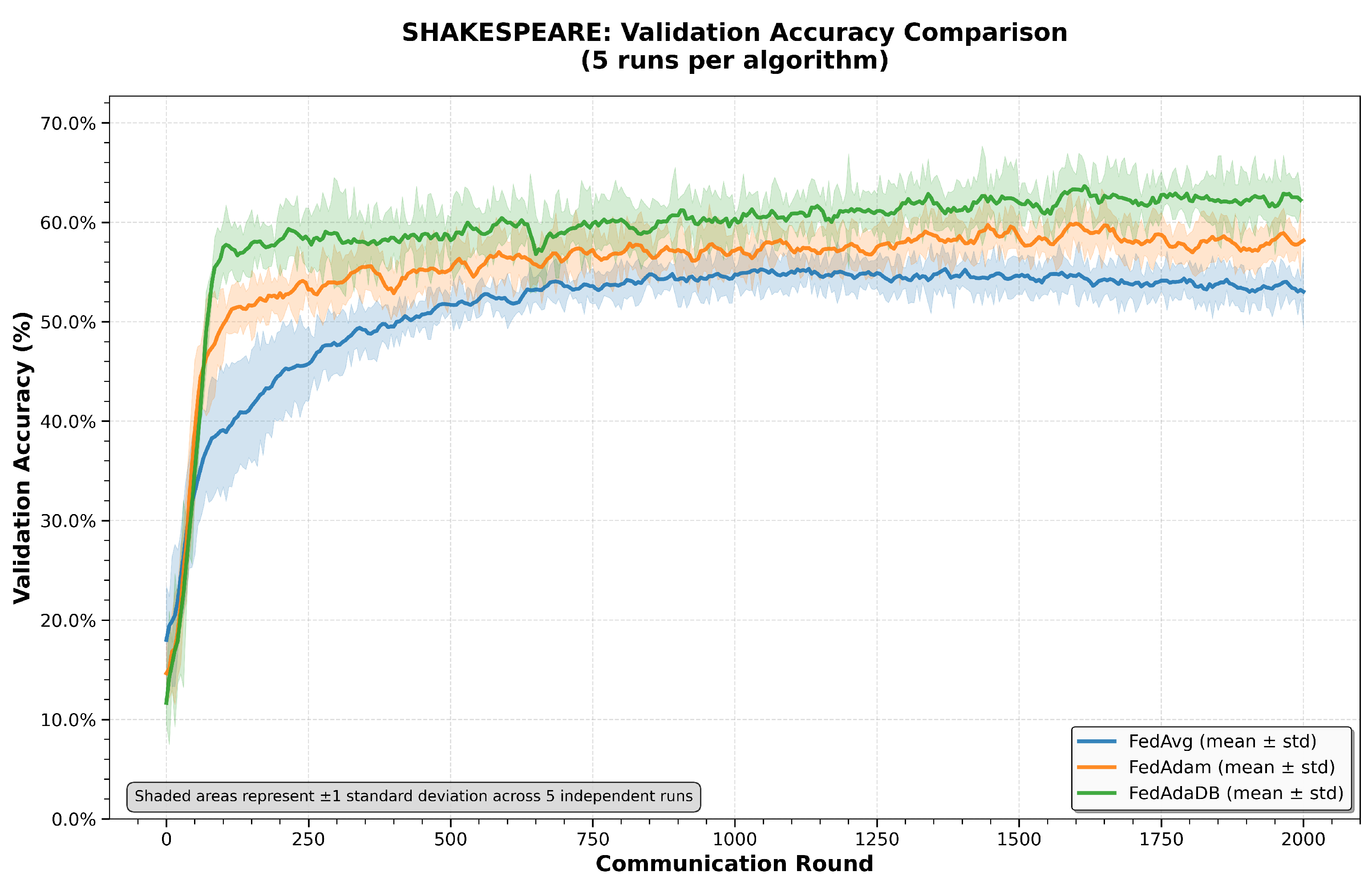
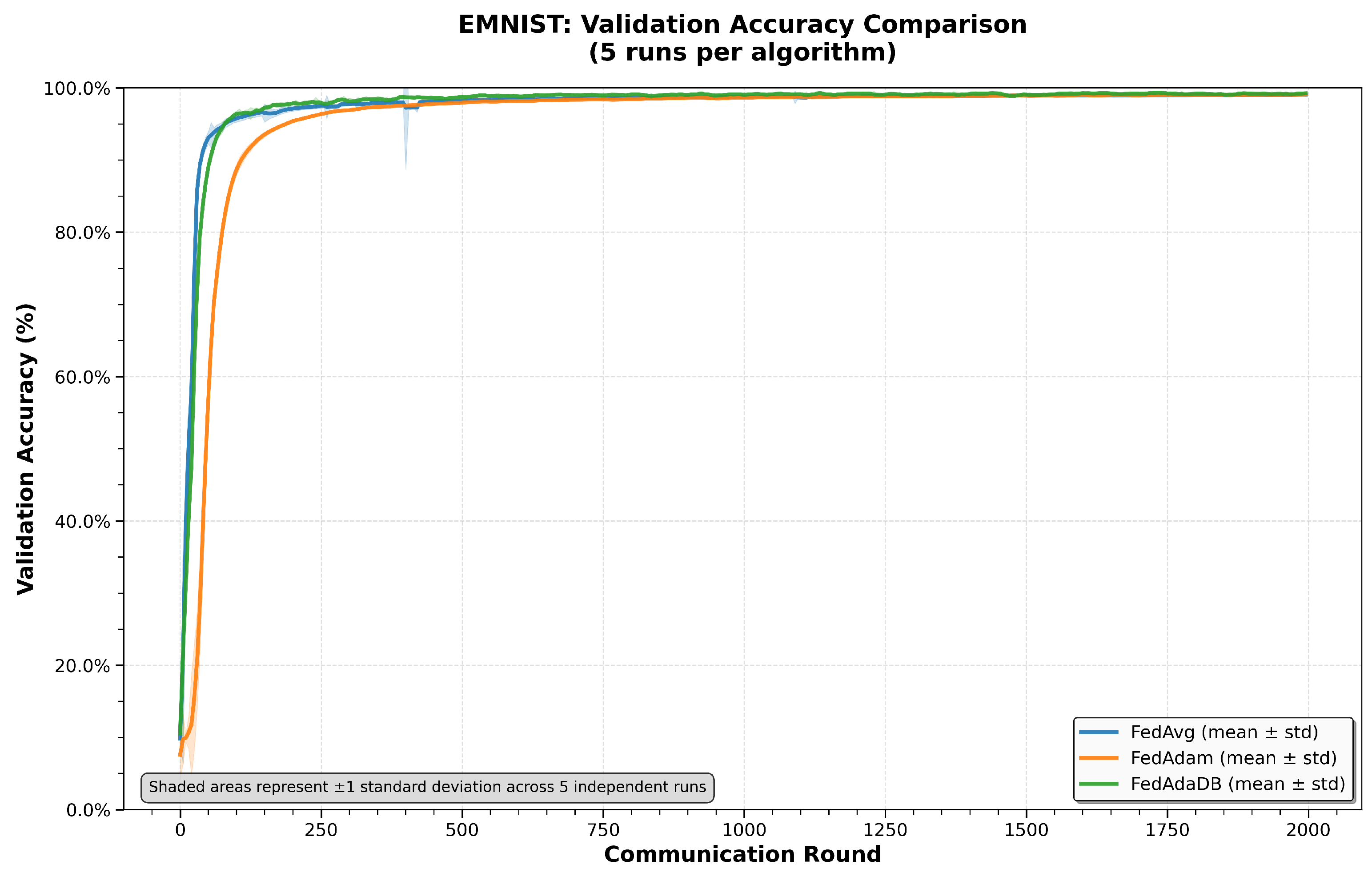
In this section, the results of the executed tests will be discussed and analyzed in depth to investigate the initial hypotheses, stating that the data-bound adaptive optimizer in the FL environment can be proven beneficial, compared to other FL algorithms, like the baseline non-adaptive FedAvg and the widely used adaptive FedAdam. The overall comparison across CIFAR100, Shakespeare, and EMNIST datasets indicates that FedAdaDB’s data-bound learning-rate clipping consistently improves validation accuracy, while also enhancing stability once a satisfactory performance level is reached. There is an apparent trade-off in the early convergence, where FedAdaDB sacrifices some convergence speed due to the clipping mechanism, which will be discussed in more detail later in this section. Moreover, paired t-tests confirm that the results are statistically significant on more challenging, heterogeneous tasks such as NCP using the Shakespeare dataset and image classification with the CIFAR100 dataset. On the other hand, on relatively easier tasks, like handwritten character recognition, using the EMNIST dataset, every algorithm performs fairly well, and FedAdaDB’s improvements are smaller and do not hold a strong statistical significance.

Regarding the final validation accuracy metric, according to Table 1, FedAdaDB demonstrates the highest average values over the last 100 rounds. These results highlight that, given enough communication rounds, server-side clipping leads to better results on the global model. While the server operates on aggregated updates rather than on raw client data, these aggregates still carry valuable information about the collective gradient landscape. FedAdaDB’s bounding technique likely mitigates the impact of divergent or noisy updates [49] stemming from client non-IID data and client drift, which can lead optimizers without clipping to converge to suboptimal solutions. The clipping prevents overly aggressive steps in the global model update, offering a more stable trajectory towards better generalizing minima, especially in complex, non-convex landscapes typical of the deep learning models used in FL. Moreover, SGD tends to achieve better generalization than Adam [50], and FedAdaDB’s data-bound clipping dictates the server optimizer to act more like Adam in the early stages and gradually move to an SGD-like behavior.

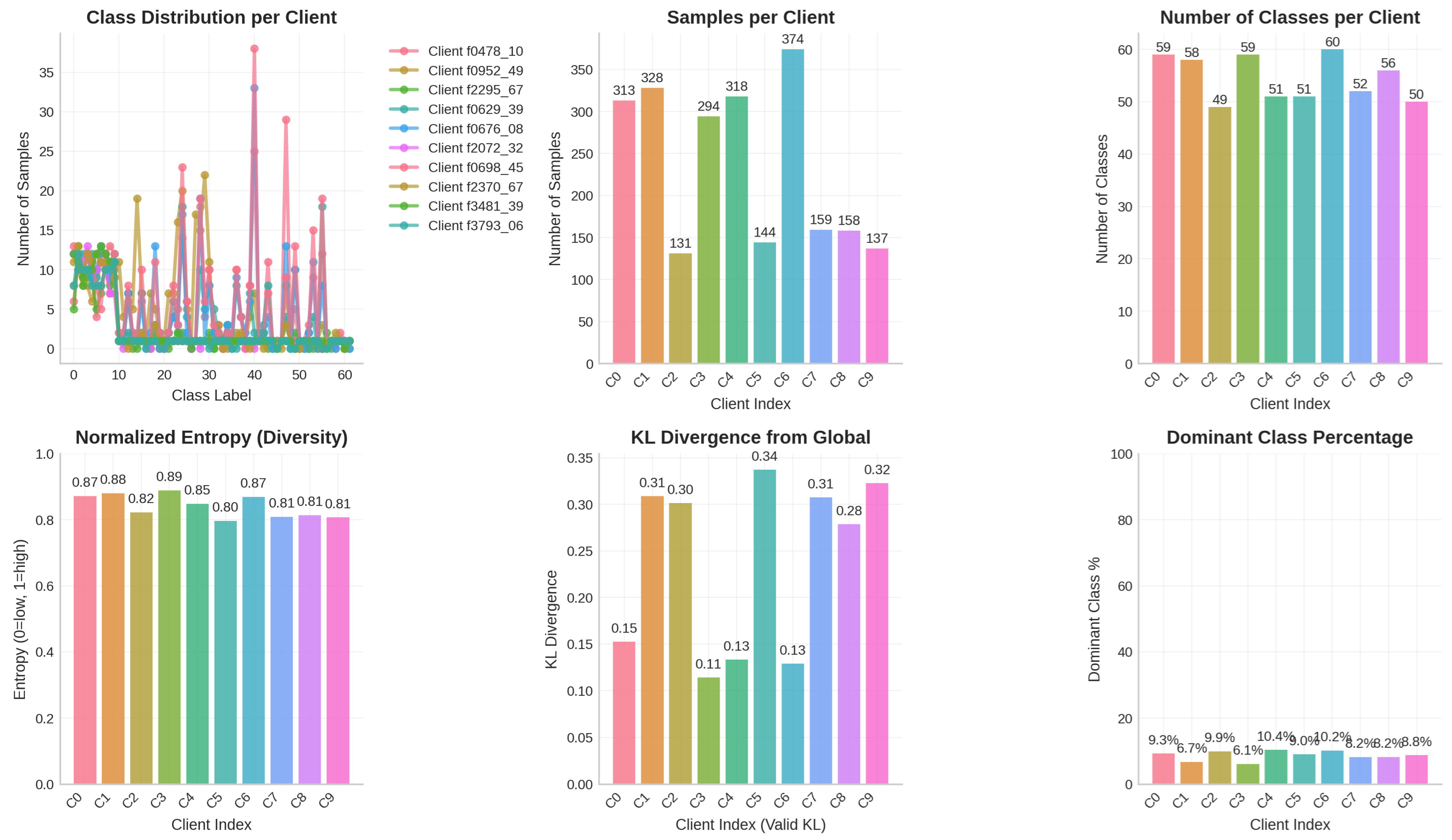
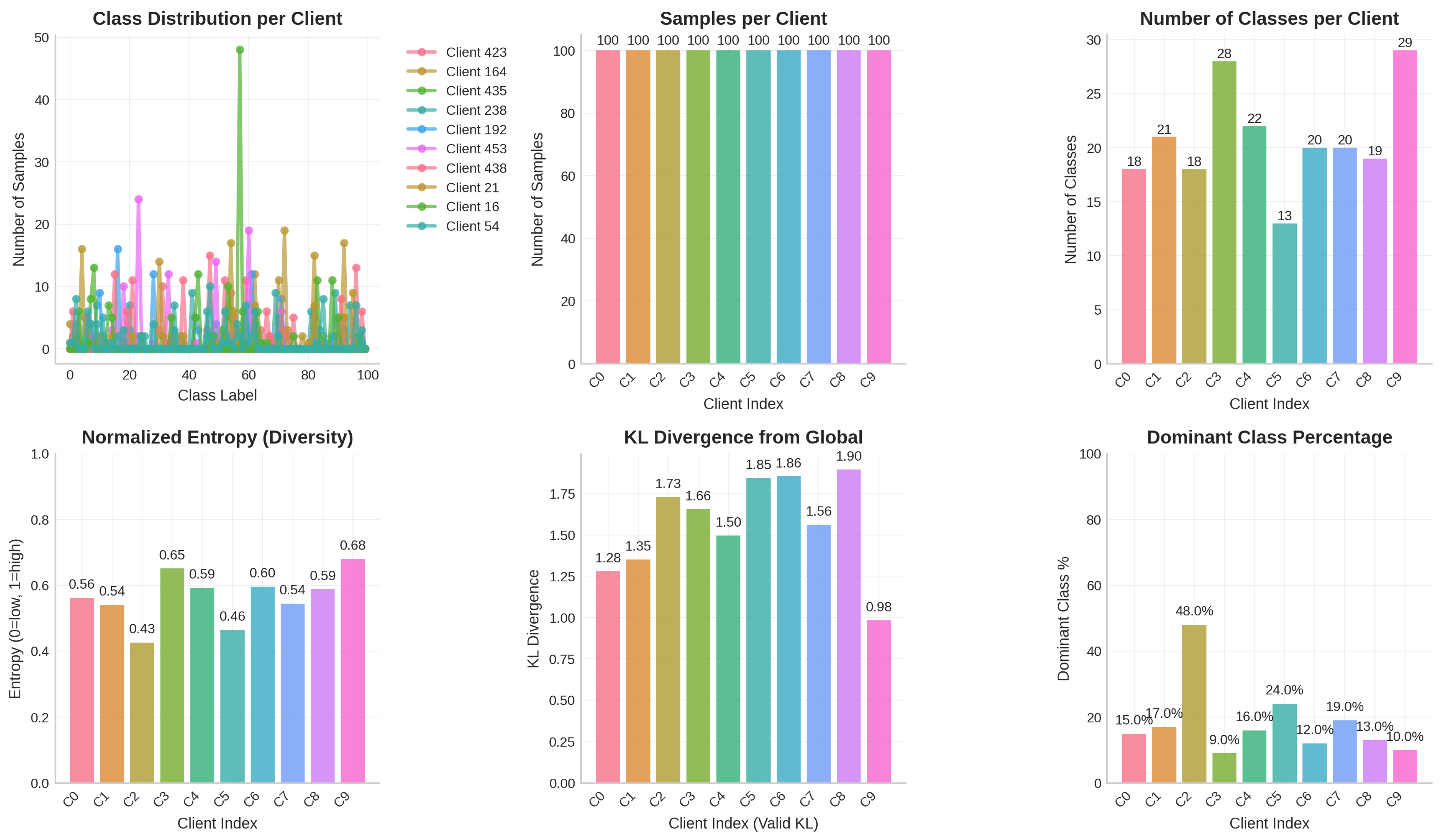
The convergence at an early stage indicates the algorithm’s convergence speed, and it is measured by the “Rounds to Threshold” metric. By examining the CIFAR100 dataset results, the FedAdaDB algorithm needs 220 rounds to reach 20% of validation accuracy, which is slower than both FedAdam and FedAvg, which require 135 and 155 rounds, respectively. The results are shifted when examining the 35% threshold where FedAdaDB requires only 565 rounds, which is significantly faster than FedAvg and even FedAdam, with 1465 and 605 rounds, respectively. As expected, FedAdaDB’s clipping mechanism has an impact on the convergence speed [17]. Clipping can lead to slower but often better convergence [51], since very large or noisy gradients are getting cut. However, after some training rounds, once past initial noise, the data-bound clipping seems to accelerate the meaningful learning. Similarly, on the EMNIST dataset, FedAdaDB needs 30 rounds to reach the 75% threshold and 45 rounds to achieve 85%, while FedAvg reaches 75% in 20 rounds and 85% in 30%. In this task, FedAdaDB outperformed FedAdam, which required 70 rounds to reach the 75% threshold and 85 rounds for the 85%. On this relatively easier task, FedAvg had an advantage and managed to converge faster since the clipping mechanism delayed FedAdaDB at the early stage. However, it offered an advantage over the FedAdam algorithm at an early stage. Finally, on the Shakespeare dataset the convergence dynamics present a different pattern. For the first threshold of 35% validation accuracy, both FedAdaDB and FedAdam demonstrate fast convergence, reaching the target in 50 rounds, surpassing FedAvg, which required 60 rounds. This suggests that, for the specific challenges of the Shakespeare dataset, characterized by significant data heterogeneity across clients [43], the stabilizing effect of FedAdaDB’s data-bound clipping might immediately counteract potential instability or excessively large gradients that could impose difficulties on other methods. The adaptive nature of both FedAdaDB and FedAdam provides an early advantage over the simpler FedAvg in the task of NCP. Moving to the higher 45% accuracy threshold, FedAdaDB achieves this in 70 rounds. While FedAdam reaches this slightly faster at 60 rounds, FedAdaDB maintains a substantial lead over FedAvg, which lags significantly, requiring 200 rounds. This indicates that while FedAdam’s adaptive learning rates might provide a slight edge in pure speed during this phase, FedAdaDB’s clipping mechanism continues to ensure robust and efficient progress. The data-bound clipping appears to achieve a good balance, preventing harmful model updates without overly restricting progress, leading to strong performance throughout the training process on this dataset.

The third metric, “Avg Acc Post-Threshold”, is an index of how stable are an algorithm’s results once the model has surpassed a satisfactory performance level. Across all datasets (Table 1, Table 2 and Table 3), FedAdaDB consistently reaches higher average accuracies post-threshold compared to FedAvg and FedAdam. In the CIFAR100 dataset, FedAdaDB attains a post-35% accuracy of 41.91%, outperforming FedAdam (38.11%) and FedAvg (35.37%). The same behavior is more apparent on Shakespeare, with a FedAdaDB average accuracy of 60.65% vs. 57.07% and 52.25% on FedAdam and FedAvg, respectively. Accordingly, on the EMNIST dataset an average of 98.89% vs. 98.82% and 98.52%. These results are strongly linked to FedAdaDB’ s adaptive gradient clipping mechanism, which gradually transitions toward a plain SGD behavior as training progresses. When the LR decays or gradients become sparse, for example, in latter training rounds of an SGD, its generalization performance is closely tied to its stability. SGD tends to maintain or improve stability under the aforementioned conditions, especially when aided by regularization, like clipping or weight decay [52]. FedAdaDB’ s design allows for aggressive adaptation in early rounds, while converging toward a more stable, SGD-like regime later. This is likely why FedAdaDB performs better in the post-threshold phase. In contrast, FedAdam, though initially fast in convergence, presents less stability in the post-threshold metric, possibly due to the adaptivity of its momentum-based updates, which may introduce some variance. FedAvg, which lacks any adaptive mechanism to regulate instability, results in consistently lower post-threshold accuracy.

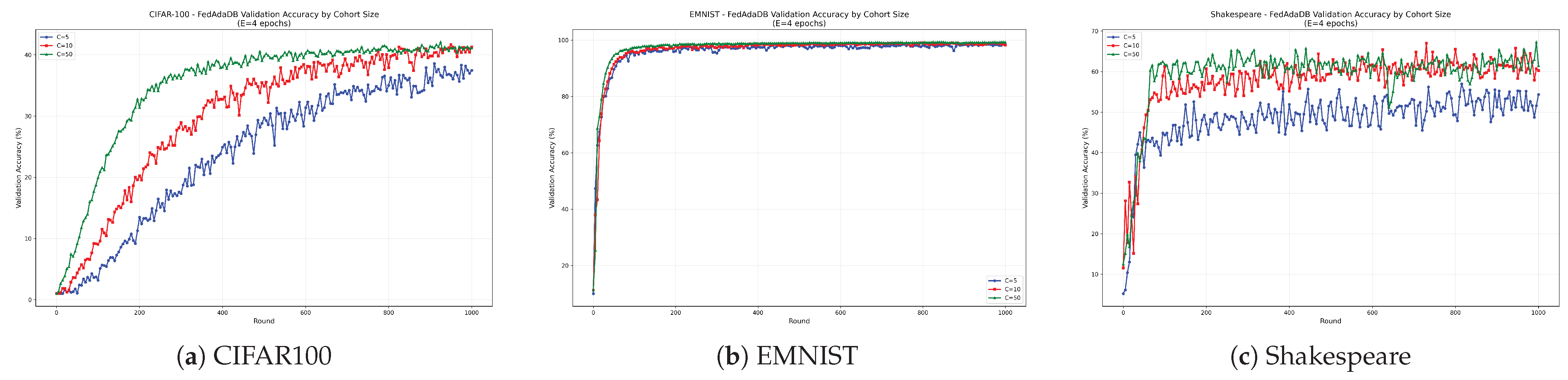
Analyzing FedAdaDB’s behavior under varying client participation levels, as presented in Figure 11, reveals that the algorithm generally benefits from larger cohort sizes, particularly on more complex datasets like CIFAR100 and Shakespeare. Increasing the number of participating clients per round (from C = 5 to C = 10 and C = 50) typically led to faster convergence and improved validation accuracy. This is aligned with the expectation that aggregating updates from a larger and more diverse set of clients per round can enhance the learning process. These findings suggest that, while FedAdaDB is robust, its convergence speed and the quality of the global model can be further optimized in practice by increasing client participation in each training round, where feasible. On the other hand, it is worth mentioning that, while increasing client participation leads to faster convergence, it has a limited impact on the final validation accuracy. Therefore, this is another trade-off that should be taken into consideration. Increasing the cohort size results in more client power consumption and increased data transfer and communication overhead. Additionally, continuously increasing the cohort size may introduce side effects such as generalization issues, diminishing returns, or catastrophic training [47].

While the empirical evidence supports the effectiveness and convergence of FedAdaDB, a formal and rigorous theoretical convergence analysis within the FL constraints and characteristics remains an important task for future investigation. Such an analysis would need to explicitly account for factors like data heterogeneity, partial client participation, and the impact of communication rounds on the convergence rate and quality. Proving that AdaDB’s convergence conditions are strictly met by the server-side optimizer using aggregated updates would solidify the theoretical concepts of FedAdaDB.

6.1. Statistical Significance

Analyzing the paired t-test results on the final validation accuracy, there seems to be a confirmation of the practical relevance of the observed improvements of FedAdaDB over the other two algorithms. Regarding the CIFAR100 dataset in Table 4, FedAdaDB against FedAdam returns a p-value of $p=2.36\times {10}^{-4}$, and against FedAvg, $p=2.32\times {10}^{-5}$. Therefore, the gains of FedAdaDB are considered significant. Similarly, on the Shakespeare dataset in Table 5, the statistical significance is also strong, with a p-value of $p=1.25\times {10}^{-2}$ when comparing FedAdaDB with FedAdam and $p=3.39\times {10}^{-5}$ when comparing with FedAvg. On the EMNIST dataset in Table 6, neither comparison crosses the typical $\alpha =0.05$ threshold (FedAdaDB vs. FedAdam $p=0.1665$; FedAdaDB vs. FedAvg $p=0.0954$), which reflects the marginal statistical importance of FedAdaDB’s improvements in a relatively easy learning task.

6.2. Limitations and Future Work

This paper demonstrates that FedAdaDB’s data-bound clipping mechanism can significantly improve the final model’s accuracy and stability when applied on the server-side optimizer. The results underlined that FedAdaDB shows a slower convergence at an early stage due to the clipping mechanism that penalizes aggressive updates. This characteristic of slower initial convergence warrants further discussion, particularly in the context of real-world FL deployments, which often suffer from communication impairments, such as packet losses or variable channel quality [53,54]. In such challenging communication environments, the slightly increased number of communication rounds that FedAdaDB might require to reach initial performance thresholds could become a more pronounced limitation. If communication rounds are frequently disrupted, delayed, or costly, an algorithm that takes longer to exhibit substantial gains in its early phases might be less practical, as each successful communication round becomes more critical. Therefore, if an application instructs that the initial convergence speed should be prioritized over the achieved final accuracy, then the selection of the most suitable server-side optimizer should be re-evaluated. Moreover, FedAdaDB architecture introduces an additional hyperparameter, the final LR ${\eta }_f$. Tuning an extra hyperparameter will increase the time and computational resources needed to achieve the ideal settings of the optimizer. Future researchers and practitioners could expand the application of the data-bound clipping mechanism to other adaptive optimizers like Yogi. Additionally, FedAdaDB could be evaluated in settings with more strict communication constraints, potentially combining it with techniques to reduce communication overhead. Techniques such as gradient sparsification or quantization have been proven to be beneficial [55]. Jump transmission is another promising approach in this domain, where only the model parameter differences are sent to the server, significantly reducing the volume of transmitted data without impacting model performance [56]. Furthermore, to more comprehensively investigate FedAdaDB’s universality and superiority, future work should include empirical comparisons against a wider range of recent federated optimization algorithms, such as FedYogi or FedLion. Such comparisons would provide deeper insights into the relative strengths of different adaptive and debiasing strategies in FL.

7. Conclusions

This paper introduced FedAdaDB, a new federated optimization algorithm that adapts the data-bound adaptive optimizer AdaDB in an FL setup and is used as the server-side optimizer. Using FedAdaDB, the server LR is dynamically clipped based on a lower and an upper bound derived from the aggregated client model updates. The goal of FedAdaDB is to improve the convergence and stability of a model in an FL setting. Through extensive experiments on the CIFAR100, Shakespeare, and EMNIST datasets, it was showcased that FedAdaDB is able to achieve statistically significant improvements in terms of the final validation accuracy, compared to the baseline FedAvg and the popular FedAdam algorithms, especially on tasks with higher complexity and data heterogeneity. While a slight delay in the initial convergence should be expected in most cases due to the clipping mechanism, FedAdaDB consistently exhibited improved performance and stability in later stages of training. The results suggest that FedAdaDB’s data-dependent clipping mechanism is effective for balancing adaptation and stability, leading to more robust and accurate global models in FL.

References

1. McMahan, B.; Moore, E.; Ramage, D.; Hampson, S.; y Arcas, B.A. Communication-efficient learning of deep networks from decentralized data. In Proceedings of the 20th International Conference on Artificial Intelligence and Statistics (AISTATS) 2017, Ft. Lauderdale, FL, USA, 20–22 April 2017; PMLR, 2017; pp. 1273–1282. Available online: https://proceedings.mlr.press/v54/mcmahan17a/mcmahan17a.pdf (accessed on 23 June 2025).
2. Yang, Q.; Liu, Y.; Chen, T.; Tong, Y. Federated machine learning: Concept and applications. ACM Trans. Intell. Syst. Technol. 2019, 10, 1–19. [Google Scholar] [CrossRef]
3. Li, L.; Fan, Y.; Tse, M.; Lin, K.Y. A review of applications in federated learning. Comput. Ind. Eng. 2020, 149, 106854. [Google Scholar] [CrossRef]
4. Zhu, H.; Xu, J.; Liu, S.; Jin, Y. Federated learning on non-IID data: A survey. Neurocomputing 2021, 465, 371–390. [Google Scholar] [CrossRef]
5. Wen, J.; Zhang, Z.; Lan, Y.; Cui, Z.; Cai, J.; Zhang, W. A survey on federated learning: Challenges and applications. Int. J. Mach. Learn. Cybern. 2023, 14, 513–535. [Google Scholar] [CrossRef]
6. Kairouz, P.; McMahan, H.B.; Avent, B.; Bellet, A.; Bennis, M.; Bhagoji, A.N.; Bonawitz, K.; Charles, Z.; Cormode, G.; Cummings, R.; et al. Advances and open problems in federated learning. Found. Trends® Mach. Learn. 2021, 14, 1–210. [Google Scholar] [CrossRef]
7. Zhang, T.; Gao, L.; He, C.; Zhang, M.; Krishnamachari, B.; Avestimehr, A.S. Federated learning for the internet of things: Applications, challenges, and opportunities. IEEE Internet Things Mag. 2022, 5, 24–29. [Google Scholar] [CrossRef]
8. Sattler, F.; Wiedemann, S.; Müller, K.R.; Samek, W. Robust and communication-efficient federated learning from non-iid data. IEEE Trans. Neural Netw. Learn. Syst. 2019, 31, 3400–3413. [Google Scholar] [CrossRef]
9. Zhang, J.; Guo, S.; Qu, Z.; Zeng, D.; Zhan, Y.; Liu, Q.; Akerkar, R. Adaptive federated learning on non-iid data with resource constraint. IEEE Trans. Comput. 2021, 71, 1655–1667. [Google Scholar] [CrossRef]
10. Reddi, S.; Charles, Z.; Zaheer, M.; Garrett, Z.; Rush, K.; Konečnỳ, J.; Kumar, S.; McMahan, H.B. Adaptive federated optimization. arXiv 2020, arXiv:2003.00295. [Google Scholar] [CrossRef]
11. Karimireddy, S.P.; Kale, S.; Mohri, M.; Reddi, S.; Stich, S.; Suresh, A.T. Scaffold: Stochastic controlled averaging for federated learning. In Proceedings of the 37th International Conference on Machine Learning, Online, 13–18 July 2020; PMLR: Cambridge, MA, USA, 2020; pp. 5132–5143. Available online: https://proceedings.mlr.press/v119/karimireddy20a.html (accessed on 23 June 2025).
12. Shi, Y.; Zhang, Y.; Xiao, Y.; Niu, L. Optimization strategies for client drift in federated learning: A review. Procedia Comput. Sci. 2022, 214, 1168–1173. [Google Scholar] [CrossRef]
13. Tang, Z.; Chang, T.H. Fedlion: Faster adaptive federated optimization with fewer communication. In Proceedings of the ICASSP 2024—IEEE International Conference on Acoustics, Speech and Signal Processing (ICASSP), Seoul, Republic of Korea, 14–19 April 2024; pp. 13316–13320. [Google Scholar] [CrossRef]
14. Jin, J.; Ren, J.; Zhou, Y.; Lyu, L.; Liu, J.; Dou, D. Accelerated federated learning with decoupled adaptive optimization. In Proceedings of the 39th International Conference on Machine Learning, Baltimore, MD, USA, 17–23 July 2022; PMLR: Cambridge, MA, USA, 2022; pp. 10298–10322. Available online: https://icml.cc/media/icml-2022/Slides/17540.pdf (accessed on 23 June 2025).
15. Wang, Y.; Lin, L.; Chen, J. Communication-efficient adaptive federated learning. In Proceedings of the International Conference on Machine Learning, Baltimore, MD, USA, 17–23 July 2022; PMLR: Cambridge, MA, USA, 2022; pp. 22802–22838. Available online: https://proceedings.mlr.press/v162/wang22o/wang22o.pdf (accessed on 23 June 2025).
16. Luo, L.; Xiong, Y.; Liu, Y.; Sun, X. Adaptive gradient methods with dynamic bound of learning rate. arXiv 2019, arXiv:1902.09843. [Google Scholar] [CrossRef]
17. Yang, L.; Cai, D. AdaDB: An adaptive gradient method with data-dependent bound. Neurocomputing 2021, 419, 183–189. [Google Scholar] [CrossRef]
18. Wu, Y.; Liu, L.; Bae, J.; Chow, K.H.; Iyengar, A.; Pu, C.; Wei, W.; Yu, L.; Zhang, Q. Demystifying learning rate policies for high accuracy training of deep neural networks. In Proceedings of the 2019 IEEE International Conference on Big Data (Big Data), Los Angeles, CA, USA, 9–12 December 2019; pp. 1971–1980. [Google Scholar] [CrossRef]
19. Wu, Y.; Liu, L. Selecting and composing learning rate policies for deep neural networks. ACM Trans. Intell. Syst. Technol. 2023, 14, 1–25. [Google Scholar] [CrossRef]
20. Wu, X.; Zhang, Y.; Shi, M.; Li, P.; Li, R.; Xiong, N.N. An adaptive federated learning scheme with differential privacy preserving. Future Gener. Comput. Syst. 2022, 127, 362–372. [Google Scholar] [CrossRef]
21. Duchi, J.; Hazan, E.; Singer, Y. Adaptive subgradient methods for online learning and stochastic optimization. J. Mach. Learn. Res. 2011, 12, 2121–2159. Available online: https://jmlr.org/papers/v12/duchi11a.html (accessed on 23 June 2025).
22. Hinton, G.; Srivastava, N.; Swersky, K. Neural Networks for Machine Learning Lecture 6a Overview of Mini-Batch Gradient Descent. 2012. Available online: https://www.cs.toronto.edu/~tijmen/csc321/slides/lecture_slides_lec6.pdf (accessed on 23 June 2025).
23. Kingma, D.P.; Ba, J. Adam: A method for stochastic optimization. arXiv 2014, arXiv:1412.6980. [Google Scholar] [CrossRef]
24. Chen, X.; Liu, S.; Sun, R.; Hong, M. On the Convergence of A Class of Adam-Type Algorithms for Non-Convex Optimization. In Proceedings of the International Conference on Learning Representations, New Orleans, LA, USA, 6– 9 May 2019; Available online: https://openreview.net/forum?id=H1x-x309tm (accessed on 23 June 2025).
25. Dozat, T. Incorporating Nesterov Momentum into Adam. In Proceedings of the 4th International Conference on Learning Representations (ICLR) Workshop, San Juan, Puerto Rico, 2–4 May 2016; pp. 1–4. [Google Scholar] [CrossRef]
26. Zaheer, M.; Reddi, S.; Sachan, D.; Kale, S.; Kumar, S. Adaptive methods for nonconvex optimization. Adv. Neural Inf. Process. Syst. 2018, 31, 9793–9803. Available online: https://papers.nips.cc/paper_files/paper/2018/hash/90365351ccc7437a1309dc64e4db32a3-Abstract.html (accessed on 23 June 2025).
27. Johnson, T.; Agrawal, P.; Gu, H.; Guestrin, C. AdaScale SGD: A user-friendly algorithm for distributed training. In Proceedings of the 37th International Conference on Machine Learning, Online, 13–18 July 2020; PMLR: Cambridge, MA, USA, 2020; pp. 4911–4920. Available online: http://proceedings.mlr.press/v119/johnson20a/johnson20a.pdf (accessed on 23 June 2025).
28. Liu, J.; Kong, J.; Xu, D.; Qi, M.; Lu, Y. Convergence analysis of AdaBound with relaxed bound functions for non-convex optimization. Neural Netw. 2022, 145, 300–307. [Google Scholar] [CrossRef]
29. Chakrabarti, K.; Chopra, N. Analysis and synthesis of adaptive gradient algorithms in machine learning: The case of AdaBound and MAdamSSM. In Proceedings of the 2022 IEEE 61st Conference on Decision and Control (CDC), Cancun, Mexico, 6–9 December 2022; pp. 795–800. [Google Scholar] [CrossRef]
30. Zhang, H.; Zeng, K.; Lin, S. FedUR: Federated learning optimization through adaptive centralized learning optimizers. IEEE Trans. Signal Process. 2023, 71, 2622–2637. [Google Scholar] [CrossRef]
31. Varno, F.; Saghayi, M.; Rafiee Sevyeri, L.; Gupta, S.; Matwin, S.; Havaei, M. Adabest: Minimizing client drift in federated learning via adaptive bias estimation. In Proceedings of the 17th European Conference on Computer Vision, Tel Aviv, Israel, 23–27 October 2022; Springer: Cham, Switzerland, 2022; pp. 710–726. [Google Scholar] [CrossRef]
32. Zhou, L.; He, Y.; Zhai, K.; Liu, X.; Liu, S.; Ma, X.; Ye, G.; Chai, H. FedCAda: Adaptive Client-Side Optimization for Accelerated and Stable Federated Learning. In Proceedings of the IEEE International Conference on Acoustics, Speech and Signal Processing (ICASSP), Hyderabad, India, 6–11 April 2025; pp. 1–5. [Google Scholar] [CrossRef]
33. Wu, X.; Huang, F.; Hu, Z.; Huang, H. Faster Adaptive Federated Learning. Proc. AAAI Conf. Artif. Intell. 2023, 37, 10379–10387. [Google Scholar] [CrossRef]
34. Lu, Z.; Pan, H.; Dai, Y.; Si, X.; Zhang, Y. Federated learning with non-iid data: A survey. IEEE Internet Things J. 2024, 11, 19188–19209. [Google Scholar] [CrossRef]
35. Hu, M.; Cao, Y.; Li, A.; Li, Z.; Liu, C.; Li, T.; Chen, M.; Liu, Y. FedMut: Generalized Federated Learning via Stochastic Mutation. Proc. AAAI Conf. Artif. Intell. 2024, 38, 12528–12537. [Google Scholar] [CrossRef]
36. Xu, H.; Li, J.; Wu, W.; Ren, H. Federated Learning with Sample-level Client Drift Mitigation. arXiv 2025, arXiv:2501.11360. [Google Scholar] [CrossRef]
37. Haldankar, A.; Riasi, A.; Nguyen, H.D.; Phuong, T.; Hoang, T. Breaking Privacy in Model-Heterogeneous Federated Learning. In Proceedings of the 27th International Symposium on Research in Attacks, Intrusions and Defenses, Padua, Italy, 30 September–2 October 2024. [Google Scholar] [CrossRef]
38. Hochreiter, S.; Schmidhuber, J. Flat Minima. Neural Comput. 1997, 9, 1–42. [Google Scholar] [CrossRef]
39. Cha, J.; Chun, S.; Lee, K.; Cho, H.C.; Park, S.; Lee, Y.; Park, S. SWAD: Domain Generalization by Seeking Flat Minima. Adv. Neural Inf. Process. Syst. 2021, 34, 22405–22418. Available online: https://proceedings.neurips.cc/paper_files/paper/2021/file/bcb41ccdc4363c6848a1d760f26c28a0-Paper.pdf (accessed on 23 June 2025).
40. TensorFlow. TensorFlow Federated. 2019. Available online: https://www.tensorflow.org/federated (accessed on 23 June 2025).
41. Cohen, G.; Afshar, S.; Tapson, J.; Van Schaik, A. EMNIST: Extending MNIST to handwritten letters. In Proceedings of the 2017 International Joint Conference on Neural Networks (IJCNN), Anchorage, AK, USA, 14–19 May 2017; pp. 2921–2926. [Google Scholar] [CrossRef]
42. Krizhevsky, A.; Hinton, G. Learning Multiple Layers of Features from Tiny Images. 2009. Available online: https://www.cs.toronto.edu/~kriz/learning-features-2009-TR.pdf (accessed on 23 June 2025).
43. Caldas, S.; Duddu, S.M.K.; Wu, P.; Li, T.; Konečnỳ, J.; McMahan, H.B.; Smith, V.; Talwalkar, A. Leaf: A benchmark for federated settings. arXiv 2018, arXiv:1812.01097. [Google Scholar] [CrossRef]
44. Wang, J.; Charles, Z.; Xu, Z.; Joshi, G.; McMahan, H.B.; Al-Shedivat, M.; Andrew, G.; Avestimehr, S.; Daly, K.; Data, D.; et al. A field guide to federated optimization. arXiv 2021, arXiv:2107.06917. [Google Scholar] [CrossRef]
45. Kundroo, M.; Kim, T. Federated learning with hyper-parameter optimization. J. King Saud Univ. Comput. Inf. Sci. 2023, 35, 101740. [Google Scholar] [CrossRef]
46. Haddadpour, F.; Kamani, M.M.; Mahdavi, M.; Cadambe, V. Local SGD with periodic averaging: Tighter analysis and adaptive synchronization. Adv. Neural Inf. Process. Syst. 2019, 32, 11082–11094. Available online: https://openreview.net/pdf?id=rkfixBHlLS (accessed on 23 June 2025).
47. Charles, Z.; Garrett, Z.; Huo, Z.; Shmulyian, S.; Smith, V. On large-cohort training for federated learning. Adv. Neural Inf. Process. Syst. 2021, 34, 20461–20475. Available online: https://openreview.net/pdf?id=Kb26p7chwhf (accessed on 23 June 2025).
48. Hsu, H.; Lachenbruch, P.A. Paired t test. In Wiley StatsRef: Statistics Reference Online; John Wiley & Sons, Ltd.: Hoboken, NJ, USA, 2014. [Google Scholar] [CrossRef]
49. Qian, J.; Wu, Y.; Zhuang, B.; Wang, S.; Xiao, J. Understanding gradient clipping in incremental gradient methods. In Proceedings of the 24th International Conference on Artificial Intelligence and Statistics, Virtual, 13–15 April 2021; PMLR: Cambridge, MA, USA, 2021; pp. 1504–1512. Available online: https://proceedings.mlr.press/v130/qian21a.html (accessed on 23 June 2025).
50. Zhou, P.; Feng, J.; Ma, C.; Xiong, C.; Hoi, S.C.H.; E, W. Towards Theoretically Understanding Why Sgd Generalizes Better Than Adam in Deep Learning. Adv. Neural Inf. Process. Syst. 2020, 33, 21285–21296. Available online: https://proceedings.neurips.cc/paper_files/paper/2020/file/f3f27a324736617f20abbf2ffd806f6d-Paper.pdf (accessed on 23 June 2025).
51. Chen, X.; Wu, S.Z.; Hong, M. Understanding gradient clipping in private sgd: A geometric perspective. Adv. Neural Inf. Process. Syst. 2020, 33, 13773–13782. Available online: https://proceedings.neurips.cc/paper/2020/file/9ecff5455677b38d19f49ce658ef0608-Paper.pdf (accessed on 23 June 2025).
52. Zhang, Y.; Zhang, W.; Bald, S.; Pingali, V.; Chen, C.; Goswami, M. Stability of sgd: Tightness analysis and improved bounds. In Proceedings of the Thirty-Eighth Conference on Uncertainty in Artificial Intelligence, Eindhoven, The Netherlands, 1–5 August 2022; PMLR: Cambridge, MA, USA, 2022; pp. 2364–2373. Available online: https://proceedings.mlr.press/v180/zhang22b/zhang22b.pdf (accessed on 23 June 2025).
53. Amiri, M.M.; Gündüz, D. Federated Learning Over Wireless Fading Channels. IEEE Trans. Wirel. Commun. 2020, 19, 3546–3557. [Google Scholar] [CrossRef]
54. Rodio, A.; Neglia, G.; Busacca, F.; Mangione, S.; Palazzo, S.; Restuccia, F.; Tinnirello, I. Federated Learning with Packet Losses. In Proceedings of the 2023 26th International Symposium on Wireless Personal Multimedia Communications (WPMC), Tampa, FL, USA, 19–22 November 2023; IEEE: Piscataway, NJ, USA, 2023; pp. 1–6. [Google Scholar] [CrossRef]
55. Jia, J.; Liu, J.; Zhou, C.; Tian, H.; Dong, M.; Dou, D. Efficient asynchronous federated learning with sparsification and quantization. Concurr. Comput. Pract. Exp. 2024, 36, e8002. [Google Scholar] [CrossRef]
56. Zhang, C.; Shan, G.; Roh, B. Communication-efficient federated multi-domain learning for network anomaly detection. Digit. Commun. Netw. 2024, in press. [Google Scholar] [CrossRef]
Figure 1. Non-IID Analysis: EMNIST Dataset (10 clients).
Iot 06 00035 g001
Figure 2. Non-IID analysis: CIFAR100 dataset (10 clients).
Iot 06 00035 g002
Figure 3. Character analysis: Shakespeare dataset (10 clients).
Iot 06 00035 g003
Figure 4. CIFAR100: Client–server ( η c η s ) learning rate tuning via grid search.
Iot 06 00035 g004
Figure 5. Shakespeare: Client–server ( η c η s ) learning rate tuning via grid search.
Iot 06 00035 g005
Figure 6. EMNIST: Client–server ( η c η s ) learning rate tuning via grid search.
Iot 06 00035 g006
Figure 7. CIFAR100 algorithms comparison: Validation accuracy over communication rounds.
Iot 06 00035 g007
Figure 8. Shakespeare algorithms comparison: Validation accuracy over communication rounds.
Iot 06 00035 g008
Figure 9. EMNIST algorithms comparison: Validation accuracy over communication rounds.
Iot 06 00035 g009
Figure 10. Box plot comparison of final validation accuracy for every dataset.
Iot 06 00035 g010
Figure 11. Validation accuracy comparison for FedAdaDB on (a) CIFAR100, (b) EMNIST, and (c) Shakespeare datasets across different cohort sizes (C = 5, C = 10, C = 50).
Iot 06 00035 g011
Figure 12. Histograms of accuracy difference for (a) FedAdaDB vs. FedAvg and (b) FedAdaDB vs. FedAdam on the CIFAR100 dataset.
Iot 06 00035 g012
Figure 13. Histograms of accuracy difference for (a) FedAdaDB vs. FedAvg and (b) FedAdaDB vs. FedAdam on the Shakespeare dataset.
Iot 06 00035 g013
Figure 14. Histograms of accuracy difference for (a) FedAdaDB vs. FedAvg and (b) FedAdaDB vs. FedAdam on the EMNIST dataset.
Iot 06 00035 g014