
Low-Memory-Footprint CNN-Based Biomedical Signal Processing for Wearable Devices †

 , ,
, , 
Abstract
1. Introduction
2. Background and Related Work
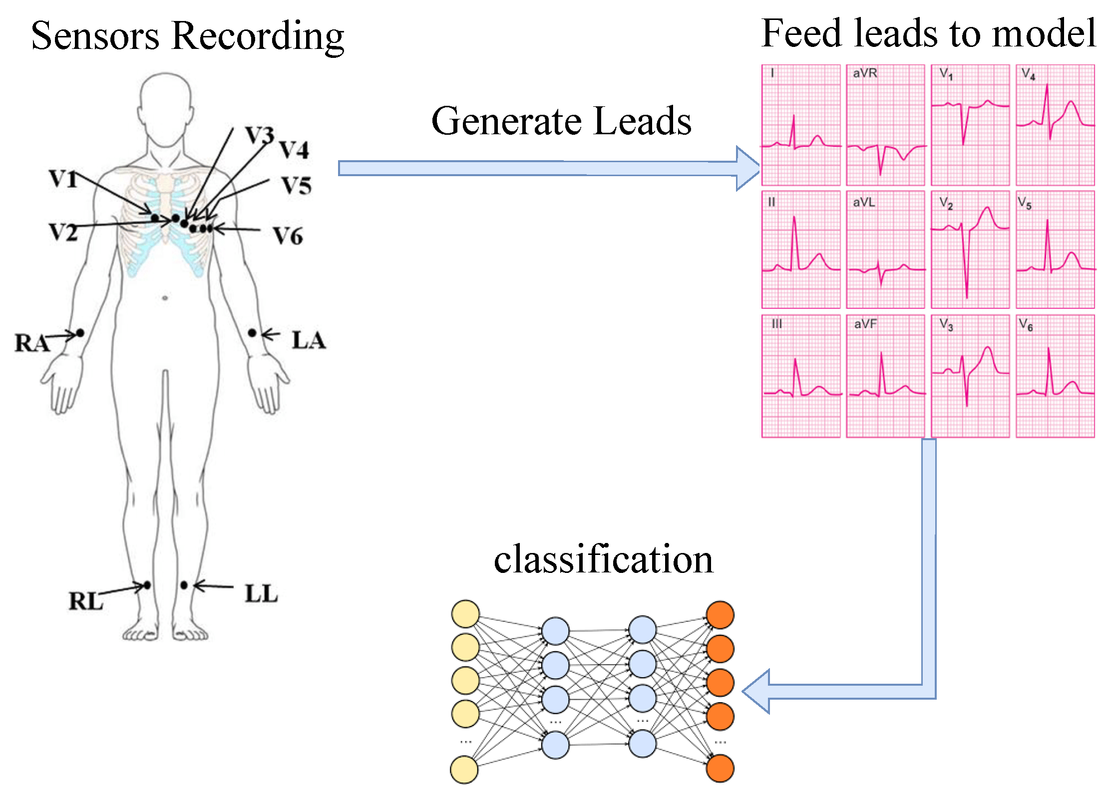
2.1. Biomedical Applications
2.2. Dataset and Preprocessing
3. CNN Compression Techniques
4. Evaluation Framework and Baseline Models
4.1. Evaluation Framework
4.2. Baseline Models
5. Investigating Alternative Model Architectures: Extracting the Lean and Fat Models
5.1. HAR Models
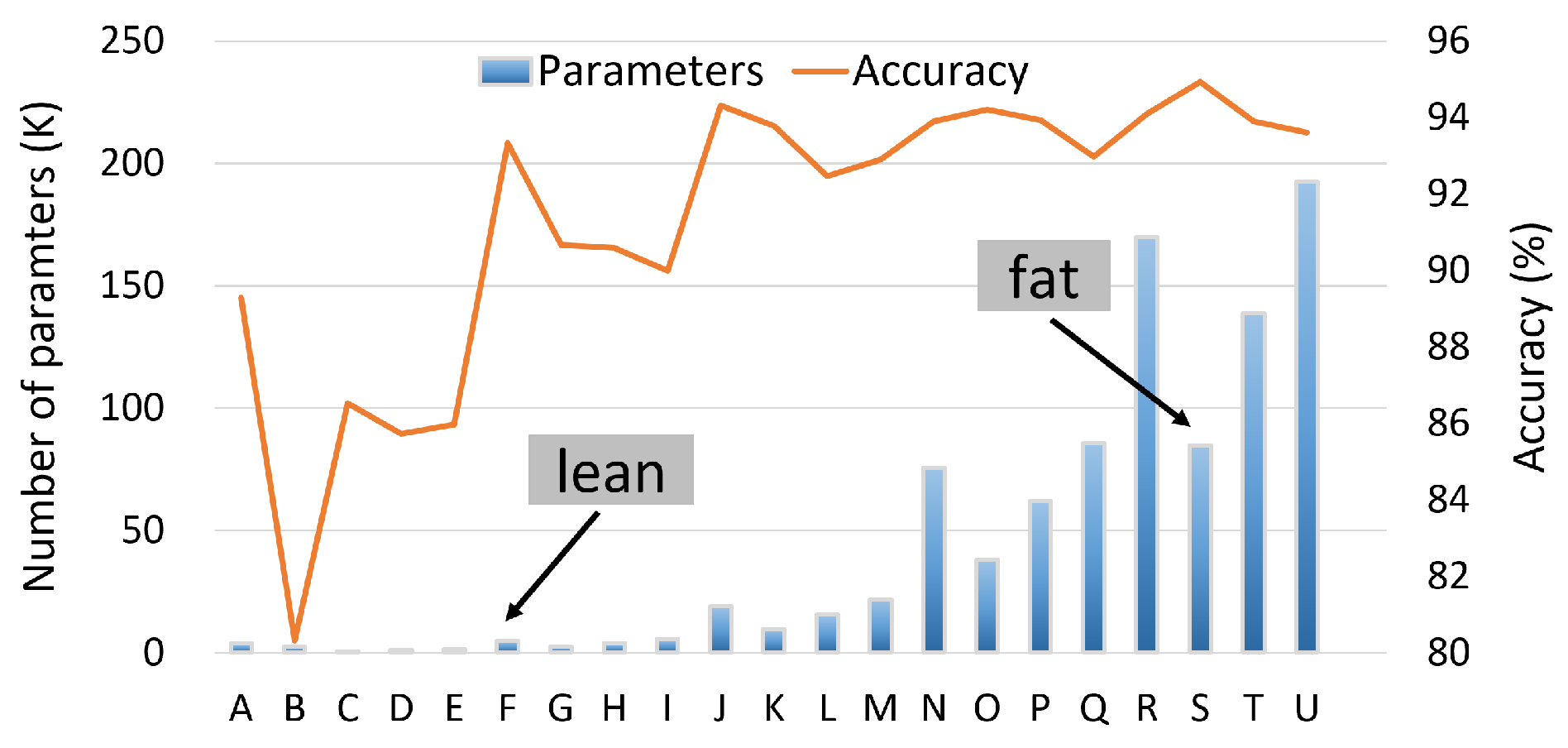
5.2. CDC Models
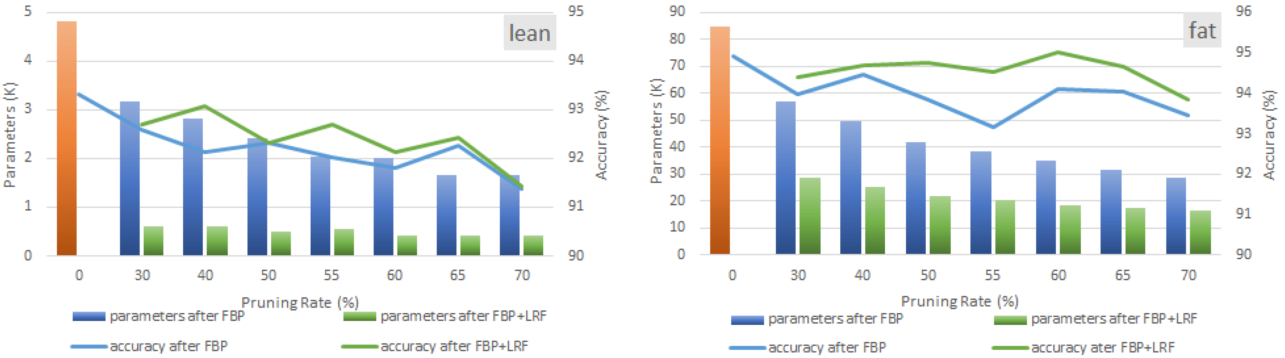
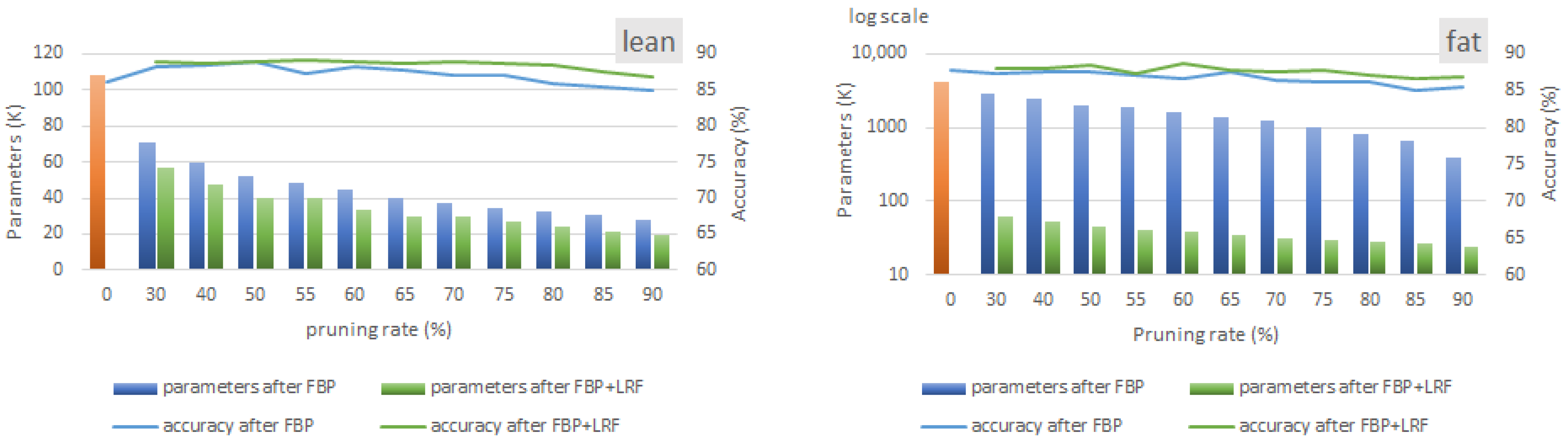
6. Synergistic Compression of Lean and Fat Models
6.1. Layer-Level Analysis
6.2. Discussion
7. Conclusions
Author Contributions
Funding
Data Availability Statement
Conflicts of Interest
References
- Number of Users of Smartwatches Worldwide from 2020 to 2029. Available online: https://www.statista.com/forecasts/1314339/worldwide-users-of-smartwatches (accessed on 15 January 2023).
- Wang, Y.; Cang, S.; Yu, H. A Survey on Wearable Sensor Modality Centred Human Activity Recognition in Health Care. Expert Syst. Appl. 2019, 137, 167–190. [Google Scholar] [CrossRef]
- Jethanandani, M.; Sharma, A.; Perumal, T.; Chang, J.R. Multi-Label Classification based Ensemble Learning for Human Activity Recognition in Smart Home. J. Internet Things 2020, 12, 100324. [Google Scholar] [CrossRef]
- Lentzas, A.; Vrakas, D. Non-Intrusive Human Activity Recognition and Abnormal Behavior Detection on Elderly People: A Review. Artif. Intell. Rev. 2020, 53, 1975–2021. [Google Scholar] [CrossRef]
- Perez, A.J.; Zeadally, S. Recent Advances in Wearable Sensing Technologies. Sensors 2021, 21, 6828. [Google Scholar] [CrossRef]
- Fitbit.com Updates. Available online: https://www.fitbit.com/global/eu/products/trackers/inspire3 (accessed on 15 January 2023).
- Abderazzak, A.; Bouattane, O.; Youssfi, M. Automatic Cardiac Cine MRI Segmentation and Heart Disease Classification. J. Comput. Med. Imaging Graph. 2021, 88, 101864. [Google Scholar]
- Neha, G.; Rathore, M.; Suman, U. MHCNLS-HAR: Multi-Headed CNN-LSTM Based Human Activity Recognition Leveraging a Novel Wearable Edge Device for Elderly Health Care. IEEE Sens. J. 2024, 24, 35394–35405. [Google Scholar]
- Dua, N.; Singh, S.N.; Semwal, V.B.; Challa, S.K. Inception Inspired CNN-GRU Hybrid Network for Human Activity Recognition. J. Multimed. Tools Appl. 2023, 82, 5369–5403. [Google Scholar] [CrossRef]
- Davide, M.; Campobello, G.; Gugliandolo, G.; Celesti, A.; Villari, M.; Donato, N. Comparison of Noise Reduction Techniques for Dysarthric Speech Recognition. In Proceedings of the 2022 IEEE International Symposium on Medical Measurements and Applications (MeMeA), Messina, Italy, 22–24 June 2022. [Google Scholar]
- Yu, J.; Zheng, X.; Wang, S. A Deep Autoencoder Feature Learning Method for Process Pattern Recognition. J. Process Control 2019, 79, 1–15. [Google Scholar] [CrossRef]
- Dargan, S.; Kumar, M.; Ayyagari, M.R.; Kumar, G. A Survey of Deep Learning and its Applications: A New Paradigm to Machine Learning. Arch. Comput. Methods Eng. 2020, 27, 1071–1092. [Google Scholar] [CrossRef]
- Hu, Z.; Zou, X.; Xia, W.; Zhao, Y.; Zhang, W.; Wu, D. Smart-DNN: Efficiently Reducing the Memory Requirements of Running Deep Neural Networks on Resource-Constrained Platforms. In Proceedings of the 2021 IEEE 39th International Conference on Computer Design (ICCD), Storrs, CT, USA, 24-27 October 2021. [Google Scholar]
- Hossain, S.M.; Islam, S.K.; Cheng, J.; Morshed, B.I. Efficient Acceleration of Deep Learning Inference on Resource-Constrained Edge Devices: A Review. Proc. IEEE 2023, 111, 42–91. [Google Scholar]
- Muck, T.; Donyanavard, B.; Moazzemi, K.; Rahmani, A.M.; Jantsch, A.; Dutt, N. Design Methodology for Responsive and Robust MIMO Control of Heterogeneous Multicores. Trans.-Multi-Scale Comput. Syst. 2018, 4, 944–951. [Google Scholar] [CrossRef]
- Suwannarat, K.; Kurdthongmee, W. Optimization of Deep Neural Network-based Human Activity Recognition for a Wearable Device. Heliyon 2021, 7, e07797. [Google Scholar] [CrossRef] [PubMed]
- Marino, G.C.; Petrini, A.; Malchiodi, D.; Frasca, M. Deep Neural Networks Compression: A Comparative Survey and Choice Recommendations. J. Neurocomput. 2023, 520, 152–170. [Google Scholar] [CrossRef]
- Kokhazadeh, M.; Keramidas, G.; Kelefouras, V.; Stamoulis, I. A Design Space Exploration Methodology for Enabling Tensor Train Decomposition in Edge Devices. In Conference in Embedded Computer Systems: Architectures, Modeling, and Simulation; Springer: Cham, Switzerland, 2022. [Google Scholar]
- Kokhazadeh, M.; Keramidas, G.; Kelefouras, V.; Stamoulis, I. Denseflex: A Low Rank Factorization Methodology for Adaptable Dense Layers in DNNs. In Proceedings of the CF ’24: 21st ACM International Conference on Computing Frontiers, Ischia, Italy, 7–9 May 2024. [Google Scholar]
- Niu, W.; Zhao, P.; Zhan, Z.; Lin, X.; Wang, Y.; Ren, B. Towards Real-Time DNN Inference on Mobile Platforms with Model Pruning and Compiler Optimization. arXiv 2020, arXiv:2004.11250. [Google Scholar]
- Gong, C.; Chen, Y.; Lu, Y.; Li, T.; Hao, C.; Chen, D. VecQ: Minimal Loss DNN Model Compression with Vectorized Weight Quantization. IEEE Trans. Comput. 2020, 70, 696–710. [Google Scholar] [CrossRef]
- Bai, S.; Kolter, J.Z.; Koltun, V. An Empirical Evaluation of Generic Convolutional and Recurrent Networks for Sequence Modeling. arXiv 2018, arXiv:1803.01271. [Google Scholar]
- Luo, J.H.; Zhang, H.; Zhou, H.Y.; Xie, C.W.; Wu, J.; Lin, W. Thinet: Pruning CNN Filters for a Thinner Net. IEEE Trans. Pattern Anal. Mach. Intell. 2018, 41, 2525–2538. [Google Scholar] [CrossRef]
- Shan, L.; Zhang, M.; Deng, L.; Gong, G. A Dynamic Multi-Precision Fixed-Point Data Quantization Strategy for Convolutional Neural Network. In Communications in Computer and Information Science; Springer: Singapore, 2016. [Google Scholar]
- He, K.; Zhang, X.; Ren, S.; Sun, J. Deep Residual Learning for Image Recognition. In Proceedings of the 2016 IEEE Conference on Computer Vision and Pattern Recognition (CVPR), Las Vegas, NV, USA, 27–30 June 2024. [Google Scholar]
- Gkountelos, D.; Kokhazadeh, M.; Bournas, C.; Keramidas, G.; Kelefouras, V. Towards Highly Compressed CNN Models for Human Activity Recognition in Wearable Devices. In Proceedings of the 2023 Signal Processing: Algorithms, Architectures, Arrangements, and Applications (SPA), Poznan, Poland, 20–22 September 2023. [Google Scholar]
- Jegan, R.; Nimi, W.S. On the Development of Low Power Wearable Devices for Assessment of Physiological Vital Parameters: A Systematic Review. J. Public Health 2023, 32, 1093–1108. [Google Scholar] [CrossRef]
- Guk, K.; Han, G.; Lim, J.; Jeong, K.; Kang, T.; Lim, E.K.; Jung, J. Evolution of Wearable Devices with Real-Time Disease Monitoring For Personalized Healthcare. J. Nanomater. 2019, 9, 813. [Google Scholar] [CrossRef]
- Laput, G.; Harrison, C. Sensing Fine-Grained Hand Activity with Smartwatches. In Proceedings of the CHI ’19: CHI Conference on Human Factors in Computing Systems, Glasgow Scotland, UK, 4–9 May 2019. [Google Scholar]
- Agarwal, P.; Alam, M. A Lightweight Deep Learning Model for Human Activity Recognition on Edge Devices. Conf. Comput. Sci. 2020, 167, 2364–2373. [Google Scholar] [CrossRef]
- Mekruksavanich, S.; Jitpattanakul, A.; Youplao, P.; Yupapin, P. Enhanced Hand-Oriented Activity Recognition based on Smartwatch Sensor Data using LSTMs. Symmetry 2020, 12, 1570. [Google Scholar] [CrossRef]
- Coelho, Y.L.; Santos, F.D.A.S.d.; Frizera-Neto, A.; Bastos-Filho, T.F. A Lightweight Framework for Human Activity Recognition on Wearable Devices. IEEE Sens. J. 2021, 21, 24471–24481. [Google Scholar] [CrossRef]
- Zebin, T.; Scully, P.J.; Peek, N.; Casson, A.J.; Ozanyan, K.B. Design and Implementation of a Convolutional Neural Network on an Edge Computing Smartphone for Human Activity Recognition. IEEE Access 2019, 7, 133509–133520. [Google Scholar] [CrossRef]
- Zhu, Y.; Mo, L. A Review of Wearable Sensor-based Human Activity Recognition using Deep Learning. In Proceedings of the 2022 International Conference on Sensing, Measurement & Data Analytics in the era of Artificial Intelligence (ICSMD), Harbin, China, 30 November–2 December 2022. [Google Scholar]
- Weiss, G.M.; Yoneda, K.; Hayajneh, T. Smartphone and Smartwatch-Based Biometrics Using Activities of Daily Living. IEEE Access 2019, 7, 133190–133202. [Google Scholar] [CrossRef]
- Ignatov, A. Real-Time Human Activity Recognition from Accelerometer Data using Convolutional Neural Networks. J. Appl. Soft Comput. 2018, 62, 915–922. [Google Scholar] [CrossRef]
- Shah, H.; Mubeen, I.; Ullah, N.; Shah, S.S.U.D.; Khan, B.A.; Zahoor, M.; Ullah, R.; Khan, F.A.; Sultan, M.A. Modern Diagnostic Imaging Technique Applications and Risk Factors in the Medical Field: A Review. BioMed Res. Int. 2022, 2022, 5164970. [Google Scholar]
- Iqbal, T.; Aaleen, K.; Ihsan, U. Explaining Decisions of a Light-Weight Deep Neural Network for Real-Time Coronary Artery Disease Classification in Magnetic Resonance Imaging. J. Real-Time Image Process. 2024, 21, 31. [Google Scholar] [CrossRef]
- Alamatsaz, N.; Tabatabaei, L.; Yazdchi, M.; Payan, H.; Alamatsaz, N.; Nasimi, F. A Lightweight Hybrid CNN-LSTM Explainable Model for ECG-based Arrhythmia Detection. J. Biomed. Signal Process. Control 2024, 90, 105884. [Google Scholar] [CrossRef]
- Mostayed, A.; Luo, J.; Shu, X.; Wee, W. Classification of 12-lead ECG signals with bi-directional LSTM network. arXiv 2018, arXiv:1811.02090. [Google Scholar]
- Moura, V.; Almeida, V.; Santos, D.B.S.; Costa, N.; Sousa, L.L.; Pimentel, P.C. Mobile Device ECG Classification using Quantized Neural Networks. J. Comput. Biol. Med. 2022. [Google Scholar] [CrossRef]
- Liu, Y.; Liu, J.; Tian, Y.; Jin, Y.; Li, Z.; Zhao, L.; Liu, C. Pruned Lightweight Neural Networks for Arrhythmia Classification with Clinical 12-Lead ECGs. J. Appl. Soft Comput. 2024, 154, 111340. [Google Scholar] [CrossRef]
- PhysioNet. Available online: https://physionet.org/ (accessed on 15 March 2023).
- The ECG Leads: Electrodes, Limb Leads, Chest (Precordial) Leads and the 12-Lead ECG. Available online: https://ecgwaves.com/topic/ekg-ecg-leads-electrodes-systems-limb-chest-precordial/ (accessed on 15 March 2023).
- Kumar, S.S.; Gupta, R. Artificial Intelligence Methods for Analysis of Electrocardiogram Signals for Cardiac Abnormalities: State-of-the-Art and Future Challenges. Artif. Intell. Rev. 2022, 55, 1519–1565. [Google Scholar]
- Sobolev, K.; Ermilov, D.; Phan, A.H.; Cickocki, A. PARS: Proxy-Based Automatic Rank Selection for Neural Network Compression via Low-Rank Weight Approximation. Mathematics 2022, 10, 3801. [Google Scholar] [CrossRef]
- Jin, H.; Wu, D.; Zhang, S.; Zou, X.; Jin, S.; Tao, D.; Liao, Q.; Xia, W. Design of a Quantization-based DNN Delta Compression Framework for Model Snapshots and Federated Learning. IEEE Trans. Parallel Distrib. Syst. 2023, 34, 923–937. [Google Scholar] [CrossRef]
- Karimzadeh, F.; Raychowdhury, A. Towards Energy Efficient DNN Accelerator via Sparsified Gradual Knowledge Distillation. In Proceedings of the 2022 IFIP/IEEE 30th International Conference on Very Large Scale Integration (VLSI-SoC), Patras, Greece, 3–5 October 2022. [Google Scholar]
- Li, D.; Wang, X.; Kong, D. Deeprebirth: Accelerating Deep Neural Network Execution on Mobile Devices. In Proceedings of the 32nd AAAI Conference on Artificial Intelligence (AAAI-18), New Orleans, LA, USA, 2–7 February 2018. [Google Scholar]
- Frusque, G.; Michau, G.; Fink, O. Canonical Polyadic Decomposition and Deep Learning for Machine Fault Detection. arXiv 2021, arXiv:2107.09519. [Google Scholar] [CrossRef]
- Oseledets, I.V. Tensor-Train Decomposition. SIAM J. Sci. Comput. 2011, 33, 2295–2317. [Google Scholar] [CrossRef]
- Novikov, A.; Izmailov, P.; Khrulkov, V.; Figurnov, M.; Oseledets, I. Tensor Train Decomposition on Tensorflow (T3F). J. Mach. Learn. Res. 2020, 21, 1–7. [Google Scholar]
- Ozen, E.; Orailoglu, A. Squeezing Correlated Neurons for Resource-Efficient Deep Neural Networks. In Machine Learning and Knowledge Discovery in Databases; Springer: Cham, Switzerland, 2021. [Google Scholar]
- Liu, Z.; Li, J.; Shen, Z.; Huang, G.; Yan, S.; Zhang, C. Learning Efficient Convolutional Networks Through Network Slimming. In Proceedings of the 2017 IEEE International Conference on Computer Vision (ICCV), Venice, Italy, 22–29 October 2017. [Google Scholar]
- TensorFlow, Post-Training Quantization. Available online: https://www.tensorflow.org/lite/performance/post_training_quantization (accessed on 1 December 2024).
- Kingma, D.P.; Adam, J.B. A Method for Stochastic Optimization. arXiv 2014, arXiv:1412.6980. [Google Scholar]
- An, A.; Kadian, T.; Shetty, M.K.; Gupta, A. Explainable AI decision model for ECG data of cardiac disorders. Biomed. Signal Process. Control 2022, 75, 103584. [Google Scholar]
- Patrick, W.; Strodthoff, N.; Bousseljot, R.D.; Kreiseler, D.; Lunze, F.I.; Samek, W.; Schaeffter, T. PTB-XL, a Large Publicly Available Electrocardiography Dataset. Sci. Data 2020, 7, 154. [Google Scholar]


| Paper | Architecture | Sensors | Parameters (Size in KB) | Preprocessing | Optimization |
|---|---|---|---|---|---|
| [29] | CNN | Accs. | 3,443,133 (13,722) | Spectrogram | - |
| [30] | LSTM | Accs. | 32,826 (131) | Segmentation | - |
| [31] | CNN+LSTM | Accs.+Gyros. | 1,677,721 (6711) | Segmentation | - |
| [32] | DT+CNN | Accs. | 5897–9113 (22.3–34.6) | Segmentation Statistical Feat. | Quantization |
| [33] | CNN | Accs.+Gyros. | 537 (2150) | Segmentation Normalization | Quantization |
| (Our work) [26] | CNN | Accs.+Gyros. | 423–16,386 (1.7–64) | Segmentation | FBP+LRF+DRQ |
| Paper | Architecture | Data Type | Parameters (Size in KB) | Preprocessing | Optimization |
|---|---|---|---|---|---|
| [38] | CNN | MRI | 507,299 (1940) | Resizing Normalization | - |
| [39] | CNN-LSTM | ECG | 40,000 (160) | Resampling Noise removal | - |
| [40] | LSTM | ECG | 52,000 (208) | Segmentation Butterworth filter | - |
| [41] | CNN | ECG | 215,500 (862) | - | Quantization |
| [42] | CNN | ECG images | 1,091,500 (4366) | - | FBP |
| Our work (res) | CNN | ECG | 62,250–66,990 (88–94) | - | FBP+LRF+DRQ |
| Our work (seq) | CNN | ECG | 19,323–27,489 (44–50) | - | FBP+LRF+DRQ |
| Model | Conv. | FC | |
|---|---|---|---|
| Width | Layers | Width | |
| A | 0.25 | 2 | 0.25 |
| B | 0.25 | 4 | 0.25 |
| C | 0.25 | 6 | 0.25 |
| D | 0.25 | 11 | 0.25 |
| E | 0.25 | 16 | 0.25 |
| F | 0.5 | 4 | 0.5 |
| G | 0.5 | 6 | 0.5 |
| H | 0.5 | 11 | 0.5 |
| I | 0.5 | 16 | 0.5 |
| J | 1 | 4 | 1 |
| K (baseline) | 1 | 6 | 1 |
| L | 1 | 11 | 1 |
| M | 1 | 16 | 1 |
| N | 2 | 4 | 2 |
| O | 2 | 6 | 2 |
| P | 2 | 11 | 2 |
| Q | 2 | 16 | 2 |
| R | 3 | 4 | 3 |
| S | 3 | 6 | 3 |
| T | 3 | 11 | 3 |
| U | 3 | 16 | 3 |
| Model | FC Width | Pooling |
|---|---|---|
| A (baseline) | 1 | Max |
| B | 0.5 | Max |
| C | 0.125 | Max |
| D | 0.0625 | Max |
| E | 0.03125 | Max |
| F | 1 | Global average |
Disclaimer/Publisher’s Note: The statements, opinions and data contained in all publications are solely those of the individual author(s) and contributor(s) and not of MDPI and/or the editor(s). MDPI and/or the editor(s) disclaim responsibility for any injury to people or property resulting from any ideas, methods, instructions or products referred to in the content. |
© 2025 by the authors. Licensee MDPI, Basel, Switzerland. This article is an open access article distributed under the terms and conditions of the Creative Commons Attribution (CC BY) license (https://creativecommons.org/licenses/by/4.0/).
Share and Cite
Kokhazad, Z.; Gkountelos, D.; Kokhazadeh, M.; Bournas, C.; Keramidas, G.; Kelefouras, V. Low-Memory-Footprint CNN-Based Biomedical Signal Processing for Wearable Devices. IoT 2025, 6, 29. https://doi.org/10.3390/iot6020029
Kokhazad Z, Gkountelos D, Kokhazadeh M, Bournas C, Keramidas G, Kelefouras V. Low-Memory-Footprint CNN-Based Biomedical Signal Processing for Wearable Devices. IoT. 2025; 6(2):29. https://doi.org/10.3390/iot6020029
Chicago/Turabian StyleKokhazad, Zahra, Dimitrios Gkountelos, Milad Kokhazadeh, Charalampos Bournas, Georgios Keramidas, and Vasilios Kelefouras. 2025. "Low-Memory-Footprint CNN-Based Biomedical Signal Processing for Wearable Devices" IoT 6, no. 2: 29. https://doi.org/10.3390/iot6020029
APA StyleKokhazad, Z., Gkountelos, D., Kokhazadeh, M., Bournas, C., Keramidas, G., & Kelefouras, V. (2025). Low-Memory-Footprint CNN-Based Biomedical Signal Processing for Wearable Devices. IoT, 6(2), 29. https://doi.org/10.3390/iot6020029