Article

Intelligent Energy Management across Smart Grids Deploying 6G IoT, AI, and Blockchain in Sustainable Smart Cities

by
Mithul Raaj A T
1,
Balaji B
1,
Sai Arun Pravin R R
1,
Rani Chinnappa Naidu
1,
Rajesh Kumar M
1,*,
Prakash Ramachandran
1,
Sujatha Rajkumar
1,
Vaegae Naveen Kumar
1,
Geetika Aggarwal
2 and
Arooj Mubashara Siddiqui
3
1
Vellore Institute of Technology, Vellore 632014, India
2
Department of Engineering, School of Computing Engineering and Digital Technologies, Teesside University, Middlesbrough TS1 3BX, UK
3
Department of Physics, Engineering and Computer Science, University of Hertfordshire, Hatfield AL10 9AB, UK
*
Author to whom correspondence should be addressed.
IoT 2024, 5(3), 560-591; https://doi.org/10.3390/iot5030025
Submission received: 28 July 2024 / Revised: 26 August 2024 / Accepted: 28 August 2024 / Published: 31 August 2024
(This article belongs to the Special Issue 6G Optical Internet of Things (OIoT) for Sustainable Smart Cities)

Abstract

:
In response to the growing need for enhanced energy management in smart grids in sustainable smart cities, this study addresses the critical need for grid stability and efficient integration of renewable energy sources, utilizing advanced technologies like 6G IoT, AI, and blockchain. By deploying a suite of machine learning models like decision trees, XGBoost, support vector machines, and optimally tuned artificial neural networks, grid load fluctuations are predicted, especially during peak demand periods, to prevent overloads and ensure consistent power delivery. Additionally, long short-term memory recurrent neural networks analyze weather data to forecast solar energy production accurately, enabling better energy consumption planning. For microgrid management within individual buildings or clusters, deep Q reinforcement learning dynamically manages and optimizes photovoltaic energy usage, enhancing overall efficiency. The integration of a sophisticated visualization dashboard provides real-time updates and facilitates strategic planning by making complex data accessible. Lastly, the use of blockchain technology in verifying energy consumption readings and transactions promotes transparency and trust, which is crucial for the broader adoption of renewable resources. The combined approach not only stabilizes grid operations but also fosters the reliability and sustainability of energy systems, supporting a more robust adoption of renewable energies.

1. Introduction

Amid a rapidly evolving global energy landscape, nations worldwide confront the pressing challenges of escalating energy demand and the imperative for sustainable development. This research proposes an innovative approach to energy management that harnesses the burgeoning capabilities of artificial intelligence, IoT, and blockchain technology to revolutionize how energy is managed, distributed, and consumed over diverse terrains. Specifically targeting developing countries like India, this project integrates solar energy into power management systems at all levels, aiming to enhance the sustainability and efficiency of these networks through the strategic application of deep learning algorithms. This integration not only optimizes energy distribution but also ensures grid stability and provides accurate forecasts of solar power generation, fostering the development of a resilient, self-optimizing energy network that supports energy independence while promoting economic stability and environmental preservation.
At the lowest level involving microgrids, the project optimizes energy management by incorporating photovoltaic energy and employing deep Q reinforcement learning to adaptively manage and allocate resources, thus enhancing efficiency and adaptability. To ensure grid stability, particularly during peak demand periods, we deployed a suite of machine learning models, including support vector machine (SVM), decision trees, extreme gradient boosting (XGBoost), and custom-built artificial neural networks (ANNs). These models are crucial in predicting and managing grid load stability, effectively preventing overloads and ensuring a consistent and reliable power supply. Enhancing this framework, predictive capabilities for solar energy generation are developed using a long short-term memory-recurrent neural network (LSTM-RNN) to analyze weather data, allowing for precise predictions of daily solar energy output. This capability helps users align their energy consumption with availability.
Complementing these AI-based technological advancements, a sophisticated visualization dashboard provides real-time, comprehensive updates and reports, aiding in strategic decision-making. The project also pioneers the use of blockchain technology, using smart contracts to authenticate energy transactions, enhancing transparency, accuracy, and trust within the renewable energy sector.
Looking toward the future, further enhancements can be realized by integrating emerging technologies such as 6G and optical IoT within this smart grid framework. The advent of 6G, with its ultra-reliable low-latency communications (URLLC) and high-speed data transfer capabilities, is poised to revolutionize how data are exchanged between sensors and control systems within smart grids. These improvements will optimize energy management systems by enabling faster and more secure data transmission, which is critical for real-time grid responsiveness and efficient energy distribution. Furthermore, optical IoT devices play a crucial role in providing precise measurements of energy consumption, generation, and storage. This precision leads to the more efficient distribution of energy resources and enhances the reliability of renewable energy systems. Together, 6G and optical IoT technologies present a transformative opportunity to advance the capabilities of smart grids, supporting the development of resilient and intelligent energy networks that can meet future demands.
This work demonstrates the transformative power of technology in shaping the future of energy. By integrating AI, IoT, blockchain, and emerging communication technologies like 6G and optical IoT, this research lays the groundwork for a resilient, intelligent energy network that supports not just energy independence but a holistic and sustainable approach to smart urban development.

2. Background

Abdul Salam [1] developed various methodologies with a focus on ANN for handling photovoltaic (PV) data’s nonlinearity. Traditional methods like linear regression are supplemented by advanced techniques such as LSTM networks and machine learning (ML) algorithms like SVM, contributing to improved forecasting accuracy and showcasing ANN’s potential for enhancing solar PV integration into the grid. Mohamed Masouddi [2] proposed grid stability using various deep learning (DL) models, where bidirectional gated recurrent unit (Bi GRU), LSTM, XGBoost, ANN, light GBM (LGBM), extreme learning machine (ELM), and quantitative assessments where performed. All model prediction accuracies were compared with the parameters R-squared (R2), root mean squared error (RMSE), and mean absolute error (MAE) values, where BiGRU and ANN were the efficient models. Abdulwahed [3] evaluated various ML models for smart grid stability prediction, including SVM, logistic regression (LR), decision tree (DT), random forest (RF), gradient-boosting trees (GBT), multilayer perceptron (MLP), gated recurrent unit (GRU), recurrent neural network (RNN), and long short-term memory (LSTM). The proposed DL model, inspired by DenseNet and ResNet, surpasses traditional classifiers, achieving up to 2.11% higher accuracy. These results of accurate smart grid stability predictions show promising resilient and efficient energy management systems. Abbhass [4] developed smart grids for better systems by implementing an ANN to forecast nodal voltage levels in the IEEE 4-bus system, comparing four ANN models. The ensemble model achieved the highest accuracy of 98.73% with mean squared error (MSE) and MAE values. Load forecasting and voltage stability through ML models like RF, SVM, and ANN show promise in power grid recovery and stability predictions. Lakhdar [5] predicted that solar power output accurately aids in efficient grid management. LSTM neural networks outperform GRU and ML models, achieving the lowest RMSE and MAE for 1 h and 2 h forecasting; LSTM consistently performs well across all seasons, demonstrating its effectiveness in solar power forecasting. Akshita [6] developed a smart grid that incorporates renewable energy stability prediction. Decentralized systems offer real-time decision-making, enhancing fault detection and self-healing capabilities. ML, particularly ANN, provides high accuracy in stability prediction. Optimization factors include hidden layer configuration, activation functions, and optimizers like Adam. ANN models achieve up to 94.63% accuracy in predicting smart grid stability. Raihanah [7] explored solar irradiance forecasting using random RF and multi-task learning (MTL) for enhanced accuracy. The integration of SWD with Daubechies wavelets effectively reduced noise, optimizing RF’s performance. Principal component analysis (PCA) was found to degrade RF’s accuracy. Through sensitivity analysis, optimal parameters of 700 trees and eight leaves were determined, refined RF’s prediction for solar irradiance forecasting. Elham [8] conducted a sensitivity analysis on the learning parameters for distributed energy resources, finding optimal strategies. Four configurations were evaluated, showing significant profit improvements with learning enabled. The results demonstrated that learning enhances agents’ adaptation and profit maximization in multi-agent environments. Zhong [9] addressed the critical need for accurate solar power forecasting due to the impact of weather uncertainties on renewable energy integration. By focusing on numerical weather prediction data, including radiation, precipitation, wind speed, and temperature, the research identifies the key weather variables influencing solar power generation. Various deep learning models are employed for forecasting, with inputs comprising historical solar power measurements and numerical weather prediction (NWP) data. Raihanah [10] proposed a forecasting technique to predict solar panel power generation, mitigating the challenges posed by intermittent solar energy. By combining a sky imagery model with a statistical approach using Raspberry Pi and LSTM, the method improves accuracy. The results show performance during rainy days, highlighting the potential of affordable hardware solutions. Expanding datasets and optimizing algorithms for broader weather conditions offers a promising avenue for microgrid solar forecasting.
Boumaiza [11] proposed a blockchain-based energy trading simulation for direct transactions between prosumers and consumers, eliminating intermediaries. Using geographic information system (GIS) data in an agent-based simulation illustrates the potential of decentralized energy trading. This aids stakeholders in understanding market dynamics and making better decisions about distributed energy resources. Sang [12] explored blockchain’s energy applications, emphasizing decentralization, security, and transparency. It supports P2P energy trading and smart metering in grid and prosumer settings and standardizes blockchain for energy, aiming at interoperability and scalability. It demonstrates blockchain’s potential to transform energy markets and grid technology adoption. Plaza [13] proposed a blockchain solution for decentralized solar energy sharing, using smart metering and a consortium blockchain with smart contracts for secure transactions. By fostering decentralized energy communities, the paper highlights blockchain’s role in governance and transitioning to renewable energy, paving the way for effective distributed energy management. Dimobi [14] suggested a Hyperledger Fabric blockchain-based model for energy exchange among residents with distributed energy resources in a 30-home microgrid. Simulations indicate a preference for auction-less schemes, particularly with diverse energy mixes, and highlight blockchain’s role in encouraging demand energy investment and improving energy efficiency in microgrid communities. Tiwari [15] evaluated the generative adversarial network (GAN), especially StyleGAN2, for NFT digital creation, gauging their suitability, merging AI with blockchain, offering fresh methods for production and verification, and benefiting artists. It outlines the pros and cons of employing GAN-generated art in NFT markets, encouraging future exploration of AI-driven art creation and its market prospects.

3. Materials and Methods

3.1. Grid-Level Stability Management

3.1.1. Methodology

The transition to smart grids, by incorporating renewable energy sources and bidirectional energy flows, demands the dynamic and precise management of grid stability. In these systems, consumer and producer roles blur as ‘prosumers’ engage in both consuming and generating electricity. The foundational step involves gathering real-time data on energy production and consumption from all nodes across the grid, leveraging advanced metering infrastructure (AMI) and IoT devices. This detailed monitoring covers not only the quantities of electricity consumed and produced but also the precise timing and rate of these activities. This is essential for maintaining an accurate power balance and identifying any discrepancies that might indicate stability issues within the grid.
Following data collection, the methodology advances to dynamic pricing and demand response management, utilizing a decentralized smart grid control (DSGC) system. This system dynamically adjusts energy prices in response to real-time supply and demand conditions, employing a mathematical model that incorporates factors such as total power balance, participant reaction times, and energy price elasticity. Consumers, informed by these real-time price signals, can adjust their energy consumption or production accordingly. This interactive process not only enhances the grid’s efficiency but also actively involves consumers in the stabilization process, allowing them to respond adaptively to changes in energy pricing.
The final phase of this methodology emphasizes ongoing monitoring and stability assessments by analyzing the grid’s frequency at various points across the network. Fluctuations in frequency are key indicators of the balance between supply and demand, making precise monitoring essential for maintaining grid stability. Machine learning algorithms and artificial neural networks [16] (ANNs) are integral to the decentralized Smart grid control (DSGC) system, which utilizes these technologies to interpret frequency data and adjust pricing strategies accordingly and continuously. When significant deviations in the frequency are detected, the system can initiate automated controls to either ramp up production at central power plants or activate specific demand response measures. These proactive adjustments help prevent instabilities and ensure the reliable operation of the grid. This advanced, data-driven approach enhances the management of the dynamic energy system, supports the broader integration of renewable energy sources, and promotes active consumer participation in energy management.

3.1.2. Datasets

The dataset [17,18] used in this project consists of 60,000 observations, simulating grid stability across a symmetric four-node star network as shown in Figure 1 below, which includes one supplier node and three consumer nodes. It contains 12 primary predictive features, which are crucial in determining the grid’s stability. The reaction times (tau1 to tau4) represent how quickly the network participants respond to changes in energy prices, with values ranging between 0.5 and 10. Specifically, tau1 corresponds to the supplier node, while tau2 through tau4 corresponds to the consumer nodes. The nominal power levels (p1 to p4) indicate the power produced by the supplier and consumed by the consumers. The supplier’s power (p1) is always positive, balancing the total power consumed by the consumers, whose values (p2 to p4) range between −2.0 and −0.5. The price elasticity coefficients (g1 to g4) measure how sensitive each node is to price changes, with values ranging from 0.05 to 1.00; g1 applies to the supplier node, while g2 through g4 applies to the consumers. The dependent variable, stabf, is a binary indicator of grid stability, categorizing each scenario as either “stable” or “unstable” based on the maximum real part of the characteristic differential equation root (stab), with stability determined when this value is less than or equal to zero.
The data points represent a variety of potential scenarios within the grid, captured through simulations based on a differential equation model representing the decentral smart grid control (DSGC) system that accounts for different configurations of reaction times, power levels, and price elasticities. This model focuses on monitoring the grid’s frequency and reacting to power imbalances caused by fluctuations in production and consumption. The comprehensive nature of this dataset makes it particularly well-suited for the development of predictive models that can accurately forecast grid stability. By examining the interplay between the various predictive features and the resulting stability classifications, researchers can gain valuable insights into the dynamics of grid stability. This, in turn, enables the development of more effective strategies for managing grid stability in real-world applications, particularly in response to changes in energy production, consumption, and pricing.

3.1.3. Algorithms

Stacking Classifier: The project utilizes a stacking classifier for classification tasks, combining the predictive power of the decision tree [19], support vector machine [20], and XGBoost [21] models. The base learners are strategically chosen for their diverse strengths: Decision trees provide intuitive decision rules and overfitting resistance with depth control; SVMs offer robust classification, which is especially effective in high-dimensional spaces; and XGBoost excels with its gradient-boosting framework that handles varied data structures efficiently. These models are stacked, with logistic regression acting as the final estimator, and are tasked with optimally integrating the individual predictions into a final decision. This ensemble method enhances the predictive performance by leveraging the unique advantages of each model, reducing the likelihood of overfitting by cross-validating predictions during training.
Artificial Neural Network (ANN): The artificial neural network (ANN) is utilized for grid stability classification and is constructed using Keras, a user-friendly high-level neural network API that is designed for quick experimentation and efficient deployment. The ANN architecture begins with an input-dense layer and includes batch normalization, which helps stabilize the activation distribution across the updates during training by reducing internal covariate shifts. To prevent overfitting, dropout layers with a rate of 0.3 are strategically placed within the network. This method randomly deactivates a subset of neurons during training, compelling the network to learn more generalized and robust features.
Bayesian optimization [22] is applied to optimize the ANN’s architecture and hyperparameters [23], using a Gaussian process (GP) as the surrogate model and expected improvement (EI) as the acquisition function. The GP model is described by the following equation:
f x ~ G P ( m x , k x , x )
where m(x) is the mean function that provides the expected value of the objective function at point x, and k(x,x′) is the covariance function or the kernel, which measures the similarity between different points x and x′ in the input space. This kernel function plays a crucial role in capturing the underlying structure of the data, allowing the GP to model complex relationships between inputs and outputs. For example, in the commonly used radial basis function (RBF) kernel, the covariance between two points decreases exponentially with their distance in the input space, meaning that closer points are expected to have more similar objective function values. The expected improvement (EI) function, which guides the search for optimal hyperparameters, is defined as:
EI ( x ) = E [ max f x f x + , 0 ]
where x+ denotes the point with the best observed objective function value so far; for instance, if the current best objective value is f(x+) = 0.8, and the GP predicts that at a new point x, the objective function f(x) might be as high as 0.85 with some uncertainty, the EI function will quantify the expected gain from sampling this new point. If the uncertainty (represented by the GP’s variance) is high, the EI might suggest exploring this new point, even if the mean prediction is close to the current best. This setup enables a balance between exploration (sampling where the uncertainty is high) and exploitation (sampling where improvement is expected). Through this method, the algorithm systematically explores different configurations of neurons and dropout rates, iteratively refining the model by evaluating its performance across various setups to identify the most effective network structure for predicting grid stability.

3.1.4. Model Development

In the model development phase, two types of models are constructed: a stacking classifier model and an artificial neural network model. The stacking classifier comprises base learners, including a decision tree, SVM, and XGBoost, with logistic regression used as the final estimator to improve prediction accuracy. The artificial neural network, built using Keras, consists of an input layer with 64 neurons, two hidden layers with 128 and 64 neurons, respectively, both employing ReLU activation, and an output layer with a single neuron using sigmoid activation. Batch normalization and dropout are incorporated to enhance model stability and prevent overfitting. Additionally, there is no requirement for data preprocessing in this phase as the dataset is complete with no missing values and is already in a suitable format for modeling. The whole process is explained in Figure 2 with a flowchart.
For the model training and validation phase, the dataset is split into training and testing subsets with an 80:20 ratio, allocating 48,000 entries for training and 12,000 for testing. This division ensures a robust training process while retaining a substantial separate set for unbiased evaluation of the model.
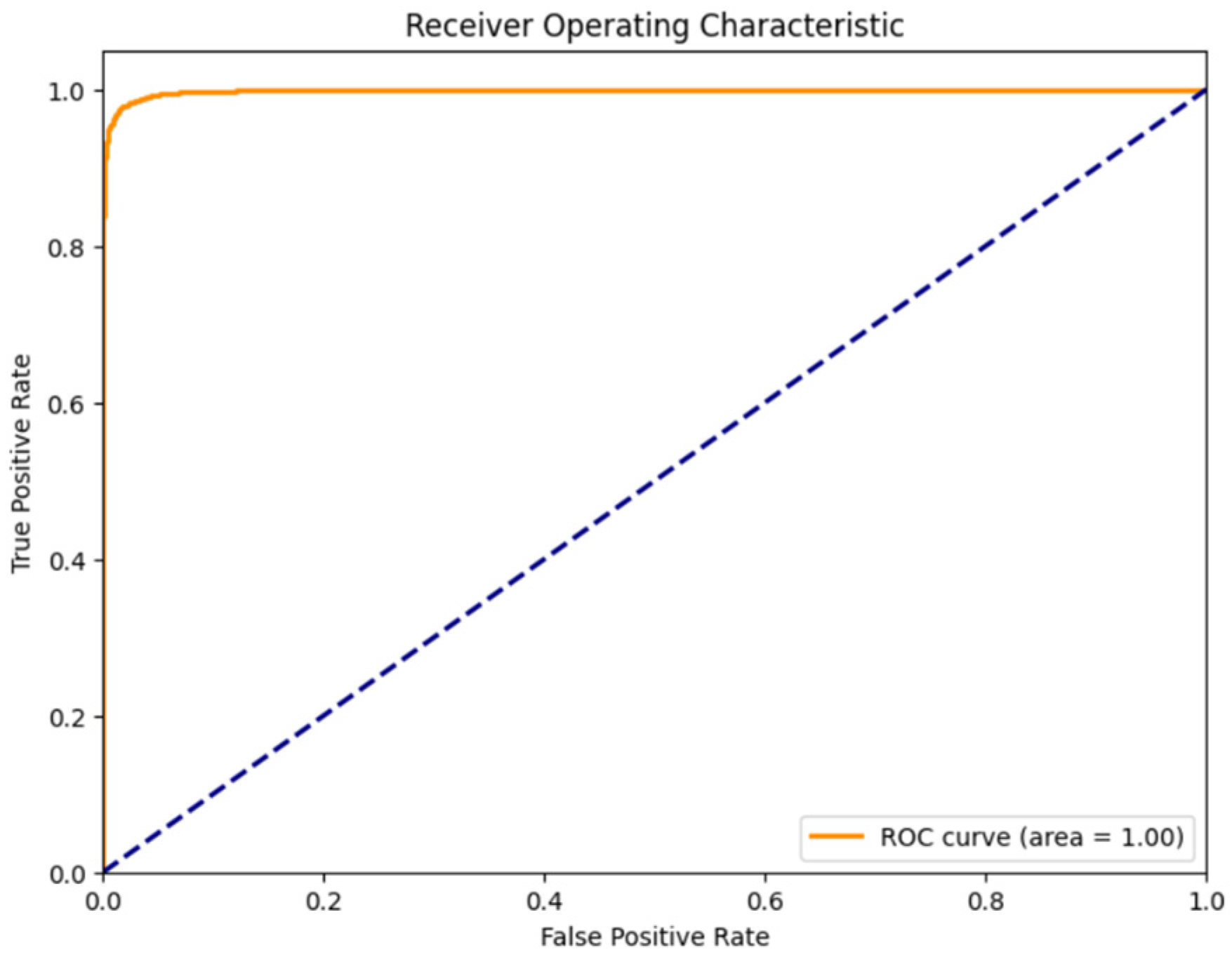
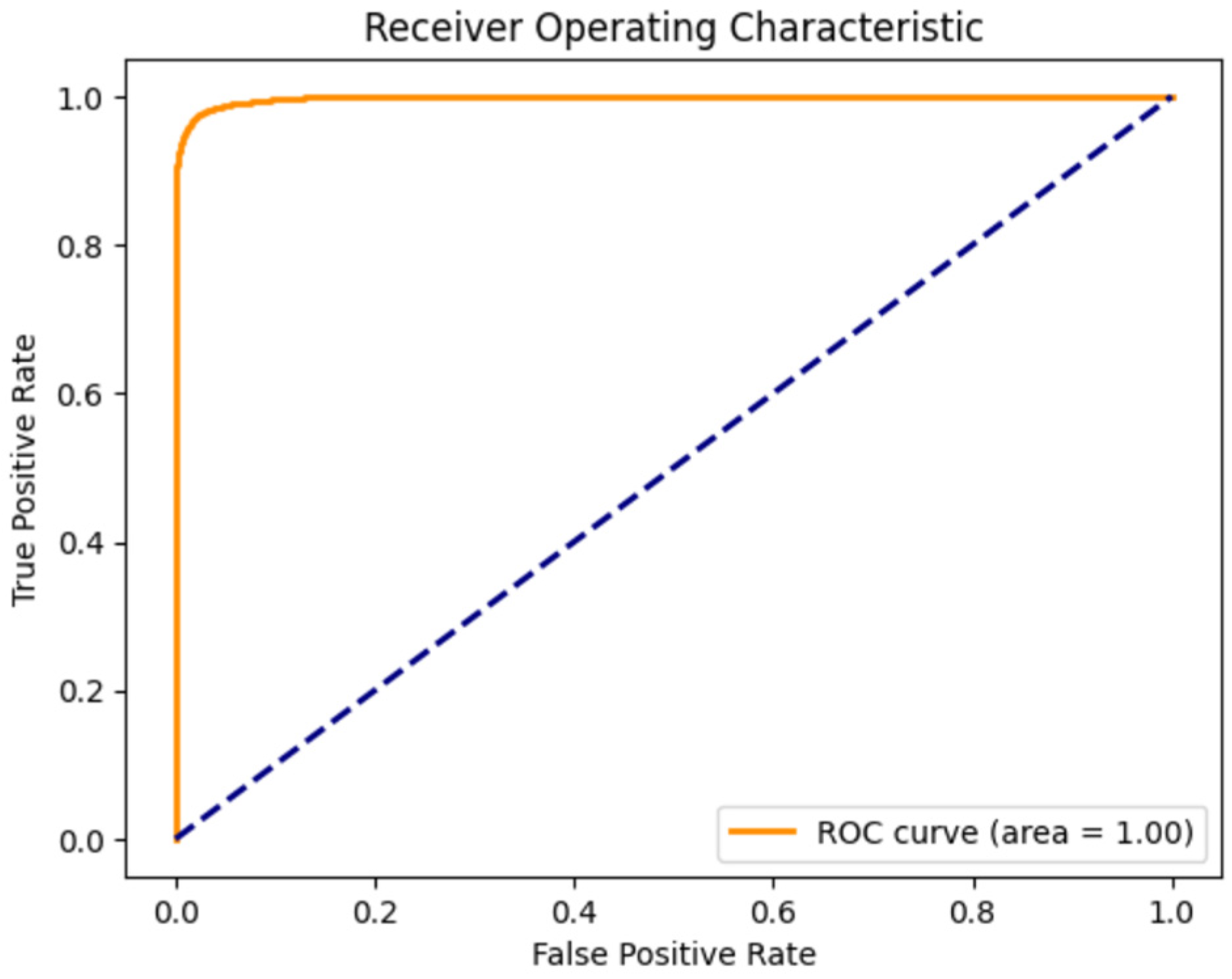
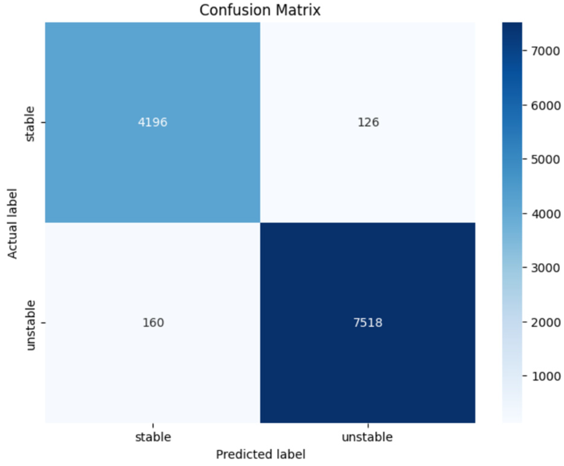
The ensemble model undergoes a meticulous training process using a 3-fold cross-validation [24] setup integrated within the stacking classifier. This strategy ensures that every data segment is used for both training and validation purposes. Such a method is critical for tuning the hyperparameters effectively and validating the model’s performance across different data subsets, thereby improving its generalizability and robustness in real-world scenarios. The final model’s effectiveness is evaluated based on accuracy, and detailed insights are provided through a classification report, ROC curve, and a confusion matrix, providing a comprehensive view of the model’s performance across various metrics. The ROC curve further illustrates the model’s ability to discriminate between classes at various thresholds, while the confusion matrix provides a clear visual of the model’s prediction accuracy across different categories. The various metrics are shown below.
Precision = T r u e   P o s i t i v e   T r u e   P o s i t i v e + F a l s e   p o s i t i v e
Recall = T r u e   P o s i t i v e   T r u e   P o s i t i v e + F a l s e   N e g a t i v e
Accuracy = T r u e   P o s i t i v e + T r u e   N e g a t i v e T r u e   P o s i t i v e + T r u e   N e g a t i v e + F a l s e   P o s i t i v e + F a l s e   N e g a t i v e
F 1 - score = 2 × P r e c i s i o n × R e c a l l P r e c i s i o n + R e c a l l
In these metrics, four terms have been used as stated: True positive (TP) occurs when the model correctly predicts a positive outcome for an instance that is actually positive; true negative (TN) is when the model correctly predicts a negative outcome for an instance that is actually negative; false positive (FP), also known as a type I error, happens when the model incorrectly predicts a positive outcome for an instance that is actually negative; false negative (FN), or type II error, occurs when the model incorrectly predicts a negative outcome for an instance that is actually positive.
Precision as shown in Formula (3) is the ratio of true-positive predictions to all predicted positives. It measures how often the model’s positive predictions are correct. Higher precision means fewer false positives. Recall as shown in Formula (4) is the ratio of true-positive predictions to all actual positives. It measures the model’s ability to identify all relevant positive instances. Higher recall means fewer false negatives. Accuracy as shown in Formula (4) is the ratio of correct predictions (true positives and true negatives) to the total number of predictions. It provides an overall measure of the model’s performance but may not be meaningful with imbalanced classes.
The F1-score as shown in Formula (5) is the harmonic mean of precision and recall, providing a single metric that balances these two aspects of model performance. The multiplication by 2 in the F1-score formula ensures that equal weight is given to both precision and recall, making it especially useful in scenarios where both false positives and false negatives are important to minimize. This balance makes the F1-score a robust measure when dealing with imbalanced datasets or when the costs of false positives and false negatives are similar.

3.1.5. Results and Discussion

Tables shows the comparative performance of the stacked ensemble method and the artificial neural network (ANN) with Bayesian optimization for grid-level classification and highlights their effectiveness in handling complex patterns inherent in grid stability datasets. The stacked ensemble method, which combines the support vector machine (SVM), decision tree, and XGBoost classifiers, achieved an overall accuracy of 0.9799, as seen in Table 1, Figure 3, Figure 4. This method also recorded high precision (0.97 for stable and 0.98 for unstable classes), recall (0.97 for stable and 0.99 for unstable classes), and the F1-score (0.97 for stable and 0.98 for unstable classes). These results indicate that the ensemble method effectively handles the complex patterns within the grid stability dataset by leveraging the strengths of each component algorithm. For instance, the decision tree mitigates overfitting through depth control, SVM excels in high-dimensional spaces, and XGBoost efficiently processes diverse data structures. The ensemble approach’s ability to combine these algorithms leads to a robust classifier with strong generalization capabilities, as reflected in the macro and weighted averages of 0.98 for precision, recall, and the F1-score.
In contrast, the ANN model, optimized using Bayesian optimization, achieved a slightly lower overall accuracy of 0.9762, as shown in Table 2, Figure 5, Figure 6. While still highly effective, the ANN’s performance metrics, including a precision of 0.96 for stable and 0.98 for unstable classes and a recall of 0.97 for stable and 0.99 for unstable classes, indicate that it falls just short of the stacked ensemble method. This slight difference in performance may be due to the challenges inherent in tuning deep learning models solely through data-driven approaches, which lack explicit feature engineering or the diverse algorithmic perspectives that ensemble methods provide. Despite this, the ANN model still showcases a strong performance, particularly in its high F1-scores (0.97 for stable and 0.98 for unstable classes), thanks to the Bayesian optimization process, which effectively balances model complexity and accuracy.
The stacked ensemble method offers a notable improvement over the ANN model, particularly in its overall accuracy and ability to generalize across different classes. This method’s strength lies in its combination of diverse algorithms—SVM, decision tree, and XGBoost—each contributing uniquely to the model’s performance. By leveraging the strengths of these individual models, the stacked ensemble provides a nuanced understanding of complex grid stability data, resulting in superior performance metrics, especially in the precision, recall, and F1-scores across both the stable and unstable classes. This integration of multiple algorithms not only surpasses the ANN in accuracy but also outperforms any single ML model, like the decision tree and random forest, in effectively classifying complex scenarios, making the stacked ensemble a more reliable and balanced approach for grid stability classification.

3.2. Solar Energy Forecasting

3.2.1. Methodology

Harnessing sunlight into electrical energy is central to solar technology as shown in Figure 7, employing either photovoltaic systems or concentrated solar power to achieve this transformation. Solar photovoltaic energy stands out as a key player in the realm of sustainable energy sources, promising a competitive edge. However, the inherent variability of solar energy production, influenced significantly by weather fluctuations such as changes in temperature and sunlight exposure, presents a notable challenge. Therefore, the project is crucially focused on the precise short-term forecasting of photovoltaic power outputs to optimize the operational efficiency of power grids and inform critical energy market strategies.

3.2.2. Dataset

Solar Power Generation Data: This dataset [25] includes detailed records from two solar power plants in India, captured over a period of 34 days. It features data from 22 inverters, with entries every 15 min, detailing the DC power output, AC power output, and cumulative energy outputs, as shown in Table 3.
Weather Sensor Data: Collected concurrently with the generation data, this dataset records ambient temperature, module temperature, and irradiation levels at 15 min intervals, as shown in Table 4. These environmental variables are critical for analyzing the impact of weather conditions on solar power output.

3.2.3. Algorithms

Random Forest (RF): This ensemble learning method uses multiple decision trees to make predictions, reducing the risk of overfitting and providing robustness against noise. In this project, it is used to predict solar power output based on input features like temperature and irradiation. Random forest [26] is valued for its ability to handle large datasets with numerous input variables without the need for extensive tuning of the hyperparameters.
Artificial Neural Network (ANN): ANNs are inspired by biological neural networks and consist of layers of interconnected nodes or neurons. Each connection can transmit a signal from one neuron to another. The receiving neuron processes the signal and signals downstream neurons connected to it. ANNs are used in this project to capture and model complex nonlinear relationships between the environmental conditions and the output power of solar panels.
  • Input Layer: The input layer consists of neurons equal to the number of features used, which, in this case, are the ambient temperature, module temperature, and irradiation. This layer serves as the entry point for data to be processed by subsequent layers.
  • First Hidden Layer: This layer has 256 neurons and uses the ReLU (rectified linear unit) activation function. ReLU is chosen for its ability to introduce nonlinearity into the model, helping to capture complex patterns in the data.
  • Dropout: A dropout rate of 30% is used after the first and subsequent batch normalization layers to prevent overfitting.
  • Second Hidden Layer: This contains 128 neurons, also with ReLU activation, further processing the inputs received from the first hidden layer.
  • Further layers follow a similar structure but gradually reduce the number of neurons (64 and 32 neurons, respectively), applying batch normalization and dropout after each layer to enhance model generalization.
  • Output Layer: The final layer is a single neuron with a linear activation function, which outputs the continuous value predicting the solar power output.
Long Short-Term Memory (LSTM): This is a special type of recurrent neural network (RNN) [27] and is capable of learning order dependence in sequence prediction problems. This is particularly useful in time-series predictions, where classical linear methods might fail. In this project, LSTM [28] networks are employed to predict the future solar energy output based on past data, leveraging their ability to remember information for long periods, which is crucial for the accurate forecasting of time-dependent variables like solar power.
  • Input Layer: This is configured to accept sequences of a specified number of past observations (n_steps), which include the same features as the ANN model. The shape of the input layer is, therefore, n_steps—the number of past observations).
  • LSTM Layer: The core of this model is an LSTM layer with 50 units. LSTM units are well-suited for time-series data because they can maintain long-term dependencies, thus remembering important information for long periods and forgetting unnecessary information.
  • Output Layer: Similar to the ANN model, the LSTM has an output layer with one neuron with a linear activation function to predict the solar power output. This setup directly maps the processed features to a predicted value.

3.2.4. Model Development

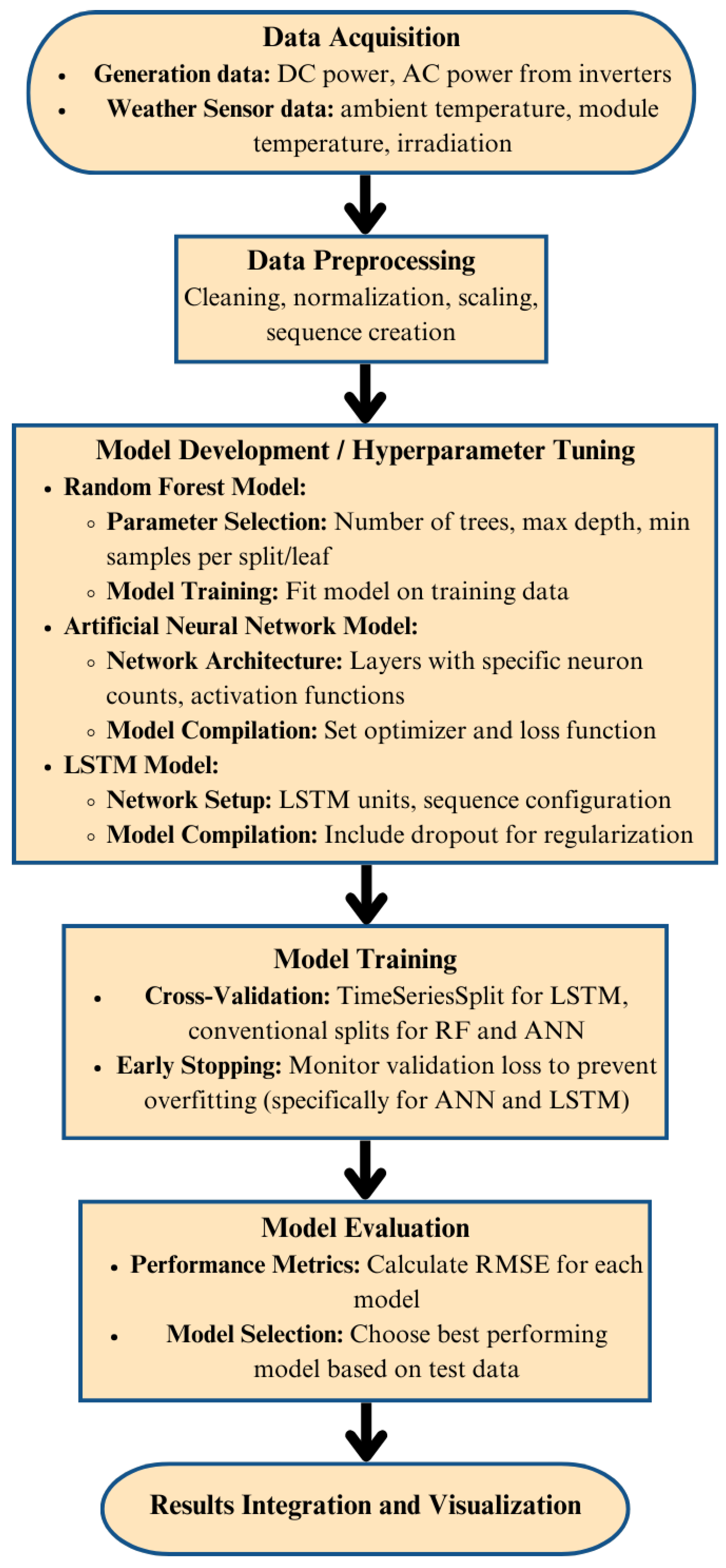
The data preprocessing stage was pivotal in shaping the raw data into a format suitable for detailed analysis and subsequent modeling. Initially, the raw datasets were cleansed of any irrelevant identifiers and corrected for any anomalies, ensuring the integrity of the data for analysis. After cleaning, the weather sensor data and generation data were merged based on their corresponding timestamps. This step was crucial to ensure that each entry in the resultant dataset accurately reflected both the environmental conditions and the corresponding solar power output at each 15 min interval. This alignment was fundamental for exploring the direct impact of weather variations on power generation. The whole process is explained in Figure 8 with a flowchart.
The normalization of features like ambient and module temperatures, along with irradiation levels, was performed using the MinMaxScaler. Additionally, for the LSTM model, a crucial preprocessing step involved transforming the time-series data into sequences. Each sequence, representing a window of past observations (n_steps), was designed to serve as input for predicting the future power output, thereby accommodating the model’s need to learn from historical data trends. The project’s model development phase involved the construction and configuration of three distinct types of predictive models, each chosen for their unique strengths in handling the dataset’s characteristics.
Model training was conducted using a designated training dataset, with careful monitoring of performance to adjust the parameters and configurations as needed. Each model underwent a series of evaluations during training to fine-tune hyperparameters, such as the number of layers in the ANN, the number of hidden units in the LSTM, and the number of trees and depth in the random forest. This hyperparameter optimization was crucial to balance each model’s complexity with its performance, ensuring effective learning without overfitting.
The validation of each model was systematically carried out using a separate set of data reserved for testing. This approach allowed for the unbiased evaluation of each model’s predictive power and generalization capabilities. Validation strategies included the use of techniques like cross-validation and early stopping. Early stopping, particularly with the ANN and LSTM, played a crucial role in preventing overtraining by halting the training process once the model’s performance on the validation set ceased to improve, thereby preserving the model’s ability to perform well on new, unseen data.
The project’s methodology involves iterative training and validation using a time-series split, which assesses the model across various sequence lengths to identify the configuration that minimizes the root mean squared error (RMSE) as shown in Formula (7). This process ensures that the LSTM model is not only tailored to the specific dynamics of the dataset but also robust against overfitting, which is facilitated by early stopping mechanisms during training. The final model, with the best number of steps, demonstrates superior predictive performance, evidenced by the low RMSE on the test data, showcasing its potential as a reliable tool in the management and optimization of solar energy systems.
RMSE = Σ i = 1 N x i x i ^ 2 N
i = variable;
N = number of non-missing data points;
x i = actual observations time series;
x i ^ = estimated time series.

3.2.5. Results and Discussion

Table 5 presents a comparative analysis of the root mean squared error (RMSE) for three different solar forecasting models used in the study. The random forest model exhibited an RMSE of 1.90884, indicating its effectiveness yet slightly less precision compared to the artificial neural network (ANN), which achieved the lowest RMSE of 1.80521, suggesting superior predictive accuracy. In contrast, the bidirectional LSTM model, while highly adept at capturing temporal dependencies, showed a higher RMSE of 2.05595, which may reflect its sensitivity to the complexities of sequential data.
Table 6, shown below, provides a detailed comparison of the actual and predicted solar power generation across three consecutive days, with hourly data spanning from 8 A.M. to 5 P.M. The columns include the date, hour of the day, actual generation in megawatts (MW), predicted generation in MW, and the percentage deviation between the actual and predicted values. The deviation percentages highlight variations in model performance, with the positive values indicating overestimations and the negative values indicating the underestimations by the predictive model.
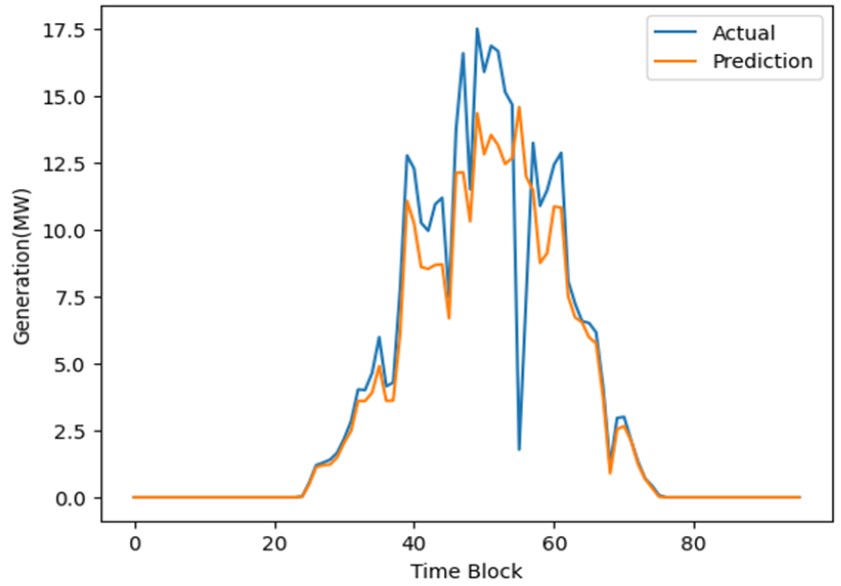
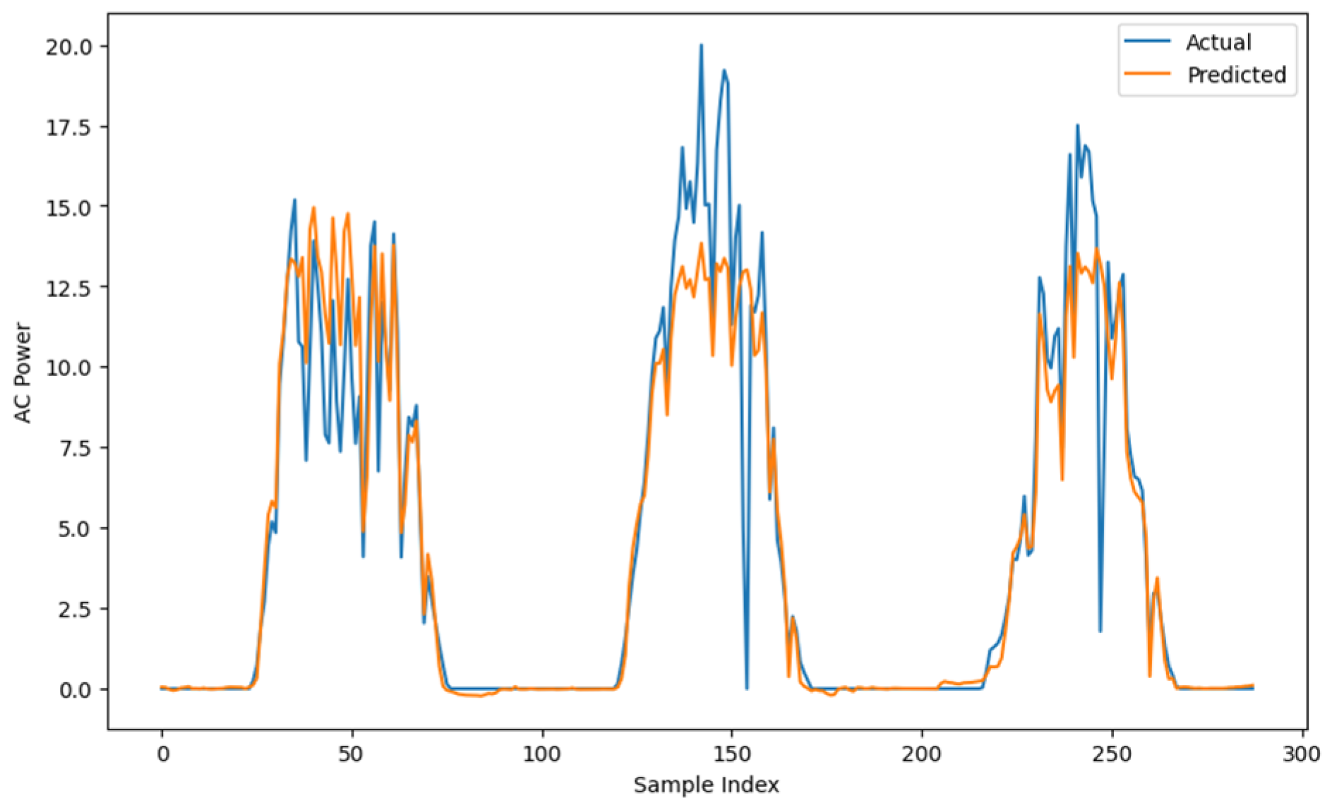
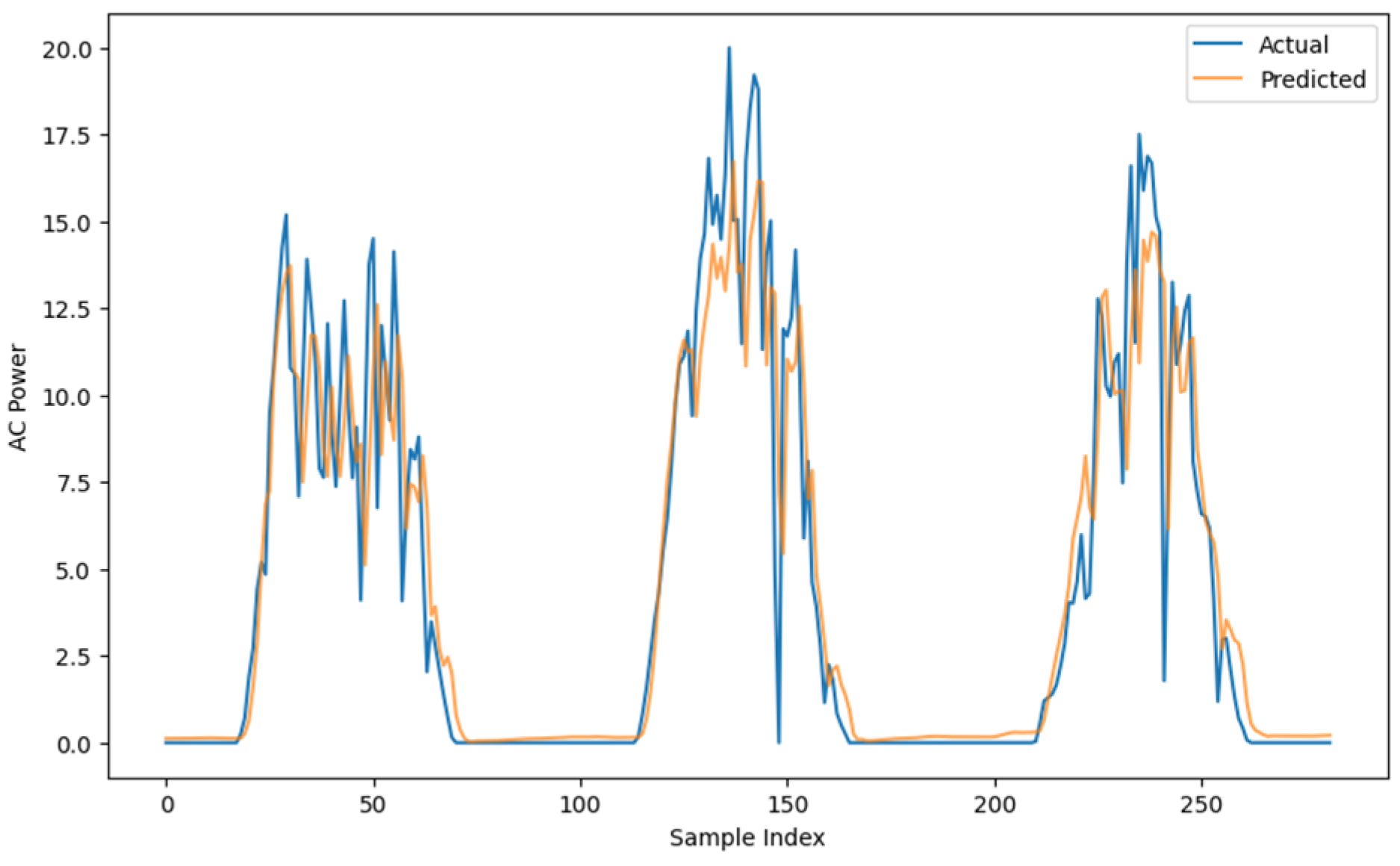
In this study, three predictive models were evaluated for their effectiveness in forecasting solar power generation: random forest as shown in Figure 9, artificial neural network (ANN) as shown in Figure 10, and bidirectional LSTM as shown in Figure 11. These figures illustrate the Actual vs Predicted AC power. Despite the LSTM model displaying a slightly higher RMSE compared to the other models, its performance in accurately capturing the variability and dynamics of solar power generation was notably superior. This observation was particularly evident from the plots, where LSTM consistently mirrored the actual energy production trends, effectively capturing both peaks and troughs. This ability is attributed to LSTM’s sophisticated architecture, which processes data sequences both forward and backward, thereby providing a comprehensive understanding of the temporal dependencies.
On the other hand, both the random forest and ANN models, while demonstrating lower RMSE values, tended to average out the prediction errors across different energy levels. This often resulted in underpredictions at higher energy levels and overpredictions at lower ones, thus not capturing the nuanced fluctuations in solar power generation as effectively as LSTM. This discrepancy suggests that while RMSE is a valuable indicator of overall predictive accuracy, it does not necessarily reflect a model’s ability to adhere to the more complex, variable patterns observed in real-world data.

3.3. Microgrid Energy Management

3.3.1. Methodology

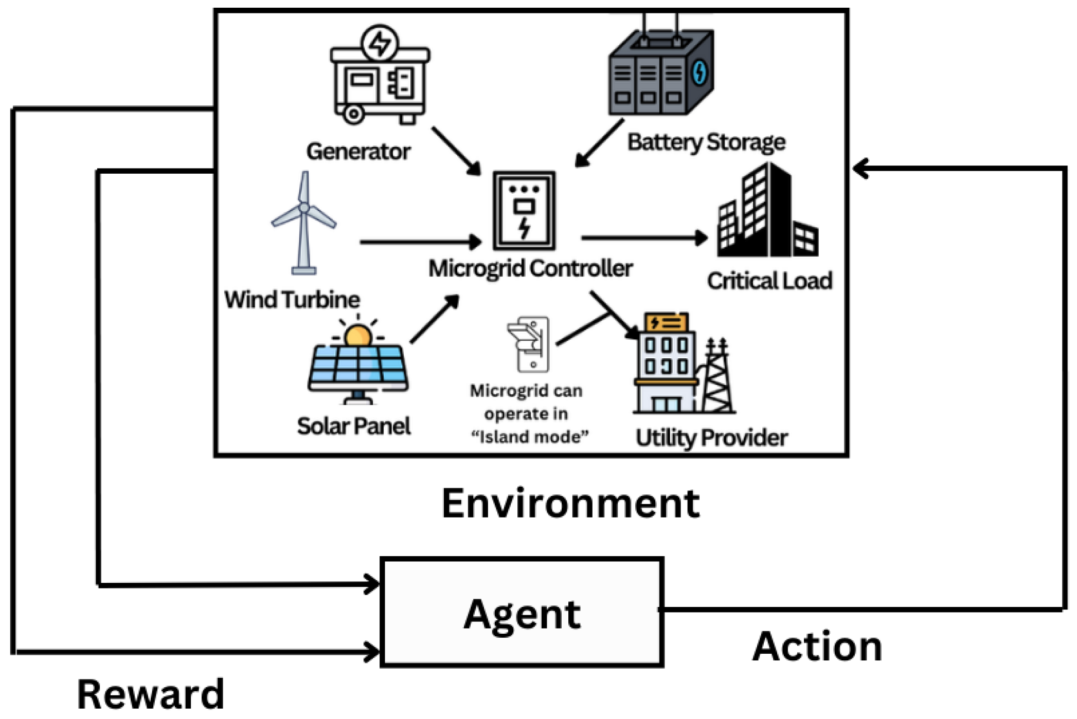
Reinforcement learning [29] is a cutting-edge machine learning approach where an agent learns to make decisions by interacting with an environment. The agent seeks to maximize cumulative rewards over time, adapting its policy based on received feedback from the environment as shown in Figure 12. This method is particularly effective in scenarios requiring complex decision-making and adaptive control, such as energy management. A fundamental challenge in reinforcement learning involves the dilemma between exploring new actions to find more rewarding strategies and exploiting known actions that yield high rewards.

3.3.2. Dataset

This dataset [31] features data with entries every 15 min, detailing the units imported from the grid, as well as the solar energy imported, stored charge, and consumed charge from the battery. The dataset provided encompasses readings from an energy management system with 30,235 observations. Table 7 details the grid electricity imports (‘grid_import’), solar power production (‘pv’), and the activity related to energy storage, and includes ‘storage_charge’ and ‘storage_decharge’, as given in the dataset. The descriptive statistics of the dataset reveal considerable variability, particularly in the photovoltaic output and grid imports, with maximum values reaching 5793.407 and 2293.708, respectively, which suggests significant fluctuations in energy production and consumption. The majority of ‘pv’ values are zero, indicating periods of no solar production, which aligns with the typical diurnal patterns or weather variability. The storage-related features (‘storage_charge’ and ‘storage_decharge’) mostly hover near zero but show occasional higher values, indicating an infrequent use or limited capacity utilization of storage systems. This dataset provides a comprehensive overview of the energy flows within a microgrid, making it crucial for optimizing and managing energy distribution and storage effectively.

3.3.3. Algorithms

Reinforcement Learning (RL): In our study, we have employed a reinforcement learning model tailored to optimize energy management within a microgrid system. This model leverages historical data on electricity imports, solar energy production, and storage behaviors to make real-time decisions aimed at enhancing energy efficiency and sustainability. The RL agent interacts with an environment that simulates the energy system, where it learns to choose actions that minimize energy costs and maximize the use of renewable sources. The framework is designed to adapt over time, improving its strategies through continuous learning and interaction with the environment, thereby ensuring it remains effective as the dynamics of the energy inputs and demands evolve. This approach not only aids in understanding optimal energy usage patterns but also contributes to the broader goal of intelligent energy management in smart grid technologies.
At the core of the DQN architecture is a neural network model that serves as the function approximator for the Q-value. The model is built using TensorFlow and Keras, leveraging a sequential model framework to facilitate the straightforward stacking of layers and clarity in the model definition. The input for this model consists of four features: grid import, photovoltaic (PV) output, storage charge, and storage decharge, reflecting the current state of the energy system.
  • Input Layer: Adjusted to receive the four features of the environment’s state.
  • Hidden Layers: Two hidden layers, each with 24 neurons, employ rectified linear unit (ReLU) activation functions. ReLU is chosen for its nonlinear properties and efficiency, allowing the model to learn complex patterns and interactions between the input features without falling into the pitfalls of gradient-vanishing problems, common with the sigmoid or tanh functions.
  • Output Layer: The final layer of the network consists of two neurons corresponding to the two possible actions: the battery discharge rate and the PV utilization rate. This layer uses a linear activation function, which directly outputs the Q-values for each possible action given the current state.
The network uses the mean squared error (MSE) as the loss function, which effectively measures the difference between the predicted Q-values and the target Q-values, providing a clear gradient for optimization. The Adam optimizer is employed for its adaptive learning rate capabilities, enhancing the convergence speed and stability of the learning process.

3.3.4. Model Development

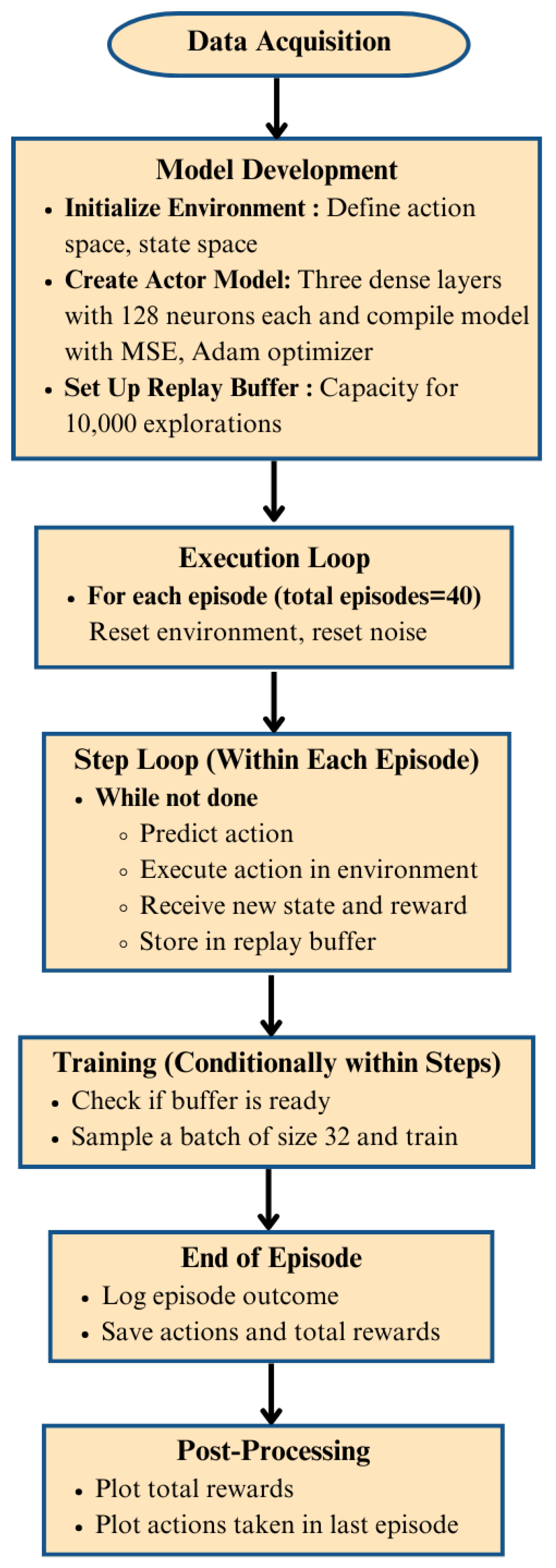
The data preprocessing for this project involves a comprehensive series of steps to ensure that the dataset is optimally prepared for use in the reinforcement learning model. The initial phase of the preprocessing involves cleaning the data, which includes addressing missing values, removing any duplicates, and correcting errors in the data entries. Although our dataset is complete with no missing values, ensuring data integrity remains a crucial step. The whole process is explained in Figure 13 with a flowchart.
Following the cleaning process, we engaged in feature selection to identify the most relevant variables for the model. For this energy management system, the selected features included ‘grid_import’, ‘pv’ (photovoltaic output), ‘storage_charge’, and ‘storage_decharge’. These features are essential for modeling the decision-making process regarding energy management. Normalization is another critical step in our preprocessing routine. Additionally, since the initial dataset presented cumulative readings for certain features, it was necessary to transform these into actual readings per time interval. This transformation was accomplished by calculating the difference between consecutive readings, thereby capturing the actual values for the energy consumed or generated in each interval.
For models that benefit from sequence understanding, like many reinforcement learning architectures, structuring the data as a time series may also be required. This structuring could involve creating lagged versions of features or reformatting the dataset so that each sequence of readings over a defined period, such as every 24 h, is treated as a single training instance. The development of the model for this energy management project involved constructing a reinforcement learning agent capable of making optimal energy usage decisions within a simulated environment. This choice is particularly relevant given the nature of energy systems, where inputs (such as power consumption and generation data) and outputs (actions like energy storage or usage) can vary in continuous ranges.
The DQN incorporates a neural network that approximates the Q-value function, a fundamental component in Q-learning that predicts the quality of a state–action combination. These actions represent various levels of battery discharge and photovoltaic (PV) utilization and are formulated as continuous values between 0 and 1. Training the DQN involves interacting with a custom-built simulation environment based on the OpenAI Gym framework. This environment reflects the dynamics of a microgrid, incorporating variables such as grid imports, PV output, and battery storage levels. As the agent operates within this environment, it learns from the consequences of its actions through a reward function designed to reduce its reliance on the grid and increase the use of stored and renewable energy. The learning process employs the epsilon-greedy strategy for action selection, balancing the need to explore new actions with the exploitation of known strategies that yield high rewards.
Experience replay is a key technique used during training to enhance learning efficiency. By storing the agent’s experiences in a replay buffer and randomly sampling from this buffer to perform updates, the method helps mitigate the risks associated with correlated data and enhances the stability of the learning algorithm. The network’s parameters are continuously updated to minimize the discrepancy between predicted Q-values and target Q-values, which are calculated using the Bellman equation as shown in Formula (8):
Q(st,at) ← Q(st,at) + α[rt+1 + γmaxaQ(st+1,a) − Q(st,at)]
where
  • Q(s,a) is the Q-value for a given state s and action a;
  • α is the learning rate;
  • rt+1 is the reward received after taking action at in state st;
  • γ is the discount factor, which weighs the importance of future rewards;
  • maxaQ(st+1,a) represents the maximum predicted Q-value in the next state across all possible actions.
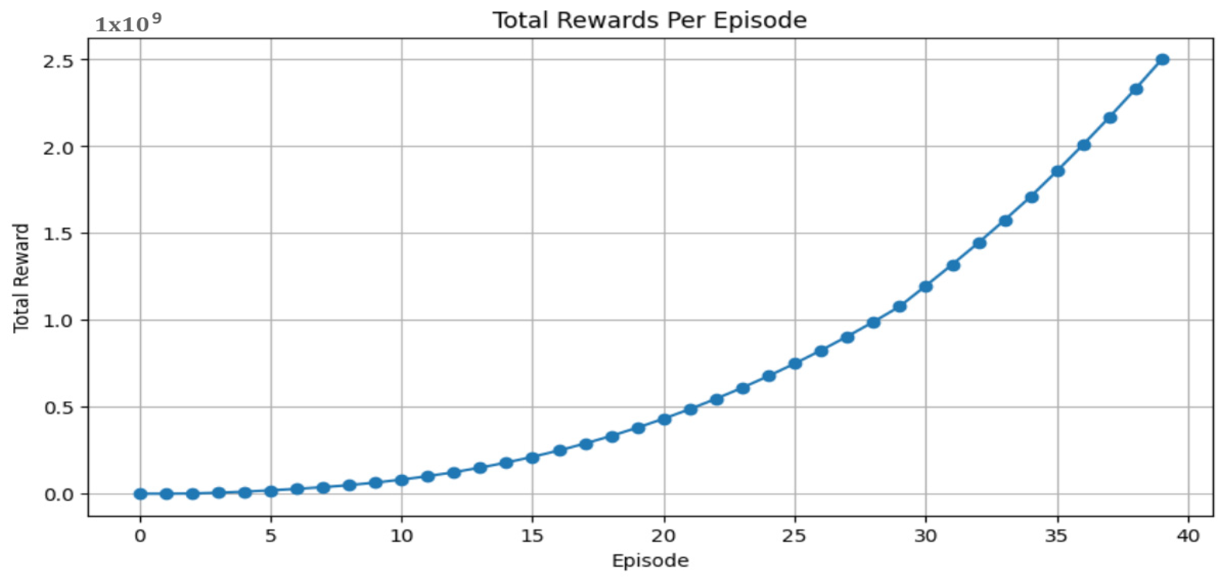
The primary method of validation for this model is through the examination of the reward and loss metrics over episodes. The rewards per episode provide an indication of how well the model is optimizing its decisions to maximize the use of photovoltaic energy while minimizing grid dependence and battery wear (through discharge cycles). An increasing trend in total rewards across the episodes typically suggests that the model is learning effective strategies for energy management.
The reward equation used in the energy management reinforcement learning model is formulated to balance the utilization of photovoltaic (PV) energy, minimize grid imports, and manage battery storage effectively. The specific reward equation implemented in the environment’s step function is
Reward = 0.1 × PV × pv_utilization − 0.1 × grid_import − 0.1 × |storage_chargedischarge|
  • PV Utilization Reward: 0.1 × PV × pv_utilization
    This term rewards the utilization of photovoltaic energy, which encourages the model to maximize the use of solar energy. The coefficient 0.1 scales the reward to ensure balance with other terms in the equation.
  • Grid Import Penalty: −0.1 × grid_import
    This term penalizes the import of energy from the grid, promoting energy independence and incentivizing the model to use locally generated solar power and stored energy. The negative sign ensures it acts as a penalty, reducing the total reward.
  • Battery Discharge Management: −0.1 × |storage_chargedischarge|
    This term penalizes excessive discharge from the battery, ensuring that the battery usage is managed efficiently and sustainability. The absolute difference between the storage charge and the discharge rate is taken to make the penalty symmetric, whether the action results in overcharging or over-discharging.
The coefficient value of 0.1 in Formula (9) was chosen to balance the competing objectives of maximizing the photovoltaic (PV) energy utilization, minimizing grid imports, and efficiently managing battery discharge in the reward function. It scales each term to prevent any one aspect from dominating the learning process, ensuring the reinforcement learning agent focuses equally on all goals. The choice of 0.1 is based on experimentation to provide stability during training, allowing the model to converge towards optimal behavior by balancing the energy efficiency and sustainability objectives effectively.
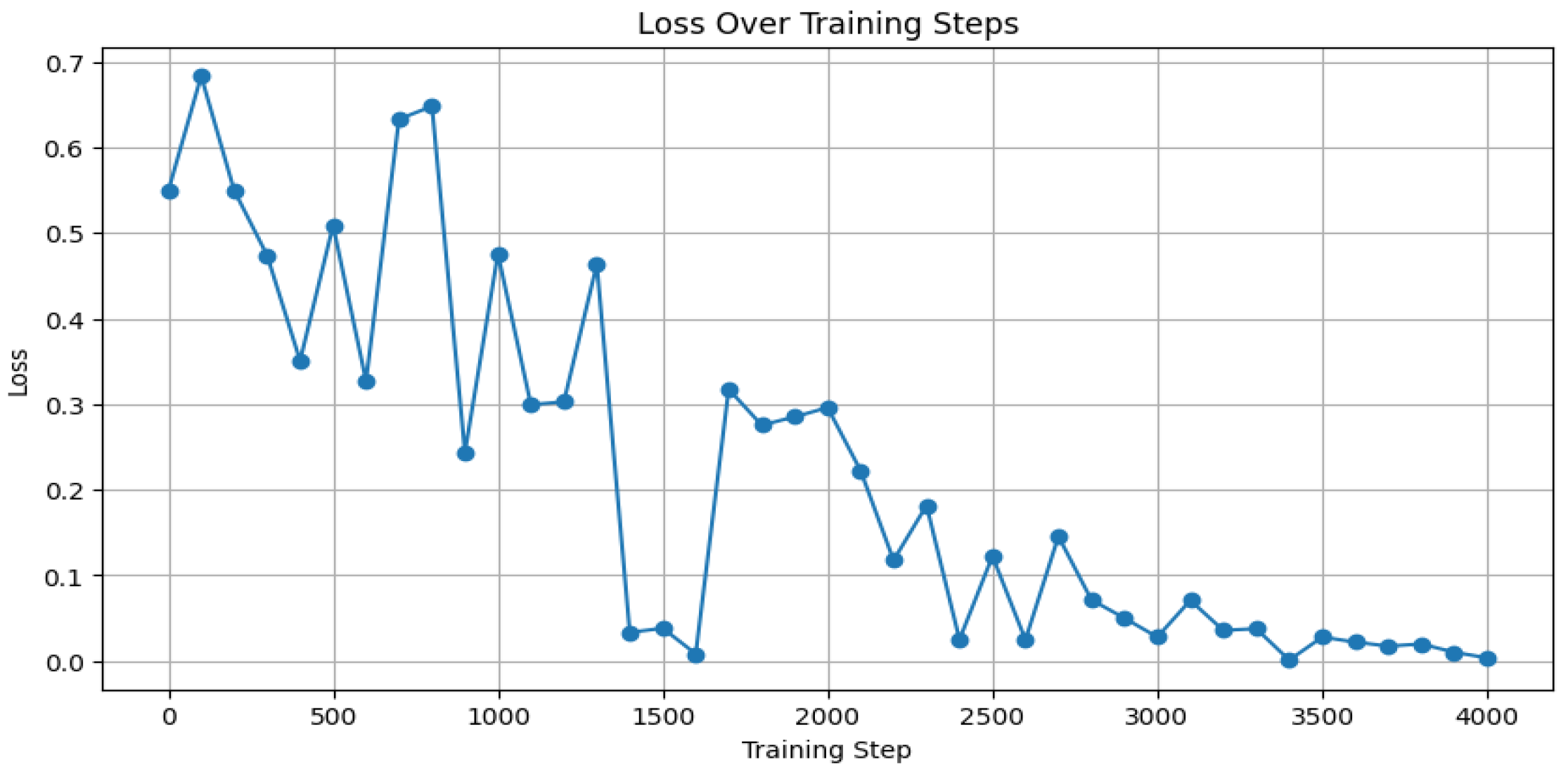
Loss metrics also play a crucial role in validation. They help in understanding how well the Q-learning model’s predictions align with the actual outcomes. A decreasing trend in loss values would indicate that the model is becoming more accurate in predicting the state–action value functions, which is fundamental to Q-learning’s success. In scenarios where the loss metrics might initially increase or fluctuate, further tuning of the hyperparameters—such as the learning rate, discount factor, or even the model architecture—may be necessary to stabilize learning and improve performance.

3.3.5. Results and Discussion

The graph as shown in Figure 14 depicting the total rewards per episode shows a clear upward trend in rewards as the number of episodes increases. This suggests that the reinforcement learning model is effectively learning and optimizing its decision-making strategy over time. As the episodes progress, the model appears to be better at balancing the use of photovoltaic (PV) power, battery storage, and grid imports to maximize rewards, which likely represents a combination of energy cost savings and efficiency.
The initial episodes exhibit relatively lower rewards, which is typical in reinforcement learning scenarios where the agent explores the environment and various actions. The significant increase in rewards in later episodes indicates that the agent has started to exploit the learned policies more effectively, leading to more optimal actions that increase the system’s overall efficiency and effectiveness.
The action distribution from the results clearly shows that the reinforcement learning (RL) agent developed for the energy management system predominantly opts to utilize stored energy, with actions frequently set at the maximum value of 1. This indicates that the agent has learned to prefer using stored energy over importing from the grid or other potential actions within the defined action space. This trend is a strong indicator of successful learning and adaptation by the agent within the simulated energy management system, achieving improved performance through continuous interaction and adjustment of its strategy based on the reward feedback. Such a performance graph is desirable, as it demonstrates that the model is not only learning but also improving in a way that aligns with the goals of minimizing energy costs and maximizing the use of renewable energy sources.
The graph as shown in Figure 15 displays the loss over training steps for the reinforcement learning model, showing a general downward trend in the loss values as training progresses. Initially, the loss fluctuates but remains relatively high, which is typical during the early stages of training, where the model explores the environment and learns from a broader range of experiences. As the training continues beyond 1500 steps, there is a noticeable decline in the loss values, indicating that the model is beginning to converge and stabilize. This reduction in loss suggests that the model’s predictions are growing closer to the actual target values, reflecting an improvement in the model’s ability to estimate the optimal actions accurately.
The decreasing trend in loss is a positive indicator of learning efficacy, suggesting that the model’s updates—guided by the chosen loss function and optimization algorithm—are effectively minimizing the prediction errors. This improvement directly contributes to the model’s ability to make decisions that lead to increased cumulative rewards, as shown in the previous reward graphs. By the end of training, the loss stabilizes at a lower level, which typically denotes that the model has learned a stable policy for the given task. This stable low loss is crucial for ensuring consistent performance when the model is deployed in real-world scenarios or continued simulations.

3.4. Interactive Data Visualization and Analytics

The dashboard provides a comprehensive visualization of electricity usage trends and patterns. It integrates multiple technologies to achieve its goals, such as the Google Cloud platform [32] (GCP) for data storage and management, Google Colab for data preprocessing and analysis, and Looker Studio [33] for creating interactive visualizations. This document outlines the technical specifications of these components and how they are used in the development of the dashboard.

3.4.1. Software Used

GCP is a comprehensive cloud computing suite that offers a range of services, from data storage to advanced analytics and machine learning. Its scalable infrastructure allows for the efficient storage and processing of large datasets, making it an ideal choice for handling complex data pipelines. Colab allows for the easy collaboration and sharing of code, making it a popular choice for data scientists and analysts. Additionally, Colab’s integration with GCP enables seamless data exchanges, providing a smooth workflow from data preprocessing to visualization.
Looker Studio, formerly known as the Google Data Studio, is a business intelligence tool designed for creating interactive data visualizations and reports. It integrates seamlessly with GCP, allowing users to access and visualize data from various sources in a highly customizable and shareable format. With Looker Studio, users can build dashboards, generate insights, and collaborate on data-driven projects. Together, GCP, Looker Studio, and Colab form a powerful ecosystem for managing, analyzing, and visualizing data in a collaborative and scalable manner.

3.4.2. Methodology

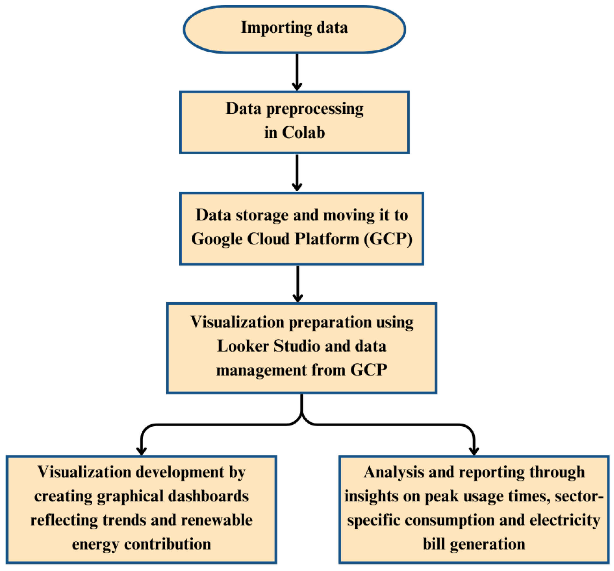
For the visualization, data are initially imported and subsequently preprocessed using Google Collaboratory (Colab), a cloud-based platform that facilitates the efficient preparation of data via a Jupyter notebook interface. The preprocessing phase is critical for ensuring the data’s suitability for advanced analytics by implementing cleaning, normalization, and transformation processes. The whole process is explained in Figure 16 with a flowchart.
A key preprocessing step was the addressing of missing values, which are examined by counting the null values in each column to identify which columns require imputation. To handle the missing values, a function called fill_nan was defined with options for forward filling (ffill), backward filling (bfill), or filling with the column mean. This flexibility allows for customization based on the data characteristics and requirements. The function is then applied to the dataset, primarily using forward-fill to address NaNs. After filling in the missing values, the filled data are saved in CSV. format and optionally as a pickle file for future use. A check for the remaining null values ensures completeness of the imputation process, providing a robust dataset for further analysis.
Post-preprocessing, the data are uploaded from Colab to the Google Cloud platform (GCP), where it is stored securely. The GCP is chosen for its robust infrastructure, which supports scalable and secure data storage solutions. This transition to the GCP is a pivotal step, ensuring that the preprocessed data are maintained in an environment that supports both high availability and integrity.
Further integration into the workflow is achieved through the use of an application programming interface (API), which facilitates access to this preprocessed data from the GCP to Looker Studio—a modern platform for data visualization and exploration. The API ensures that any updates to the data stored on the GCP are automatically synchronized with Looker Studio. This dynamic link means that the visualizations and dashboards in Looker Studio are always current, reflecting the most recent data without manual updates.
In the subsequent phase of the project, Looker Studio is utilized to develop detailed graphical dashboards. These dashboards effectively visualize the trends and contributions from renewable energy sources, offering stakeholders intuitive and actionable insights. This visualization capability is essential for discerning complex data patterns and fostering an understanding of key operational metrics.
The final stage of the project involves comprehensive analyses and reporting, where insights on the peak usage times, sector-specific consumption, and the generation of electricity bills are derived. The API’s real-time data integration allows these analyses to be continuously updated, providing stakeholders with the latest information for decision-making.

3.4.3. Results and Discussions

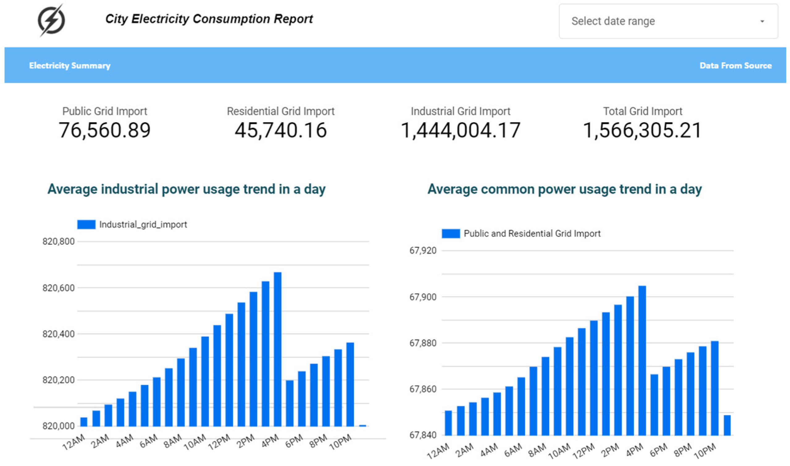
In the dashboard as shown in Figure 17, the three grids, the public grid, residential grid, and industrial grid, are displayed. The industrial sector accounts for a significant 92 percent of the total grid imports. Analyzing the average industrial power usage trend in a day, we can see a spike in the grid imports between 12 p.m. and 4 p.m. Similarly, in the “Average Common Power Usage Trend in a Day” graph, public and residential grid imports peak between 2 p.m. and 4 p.m.
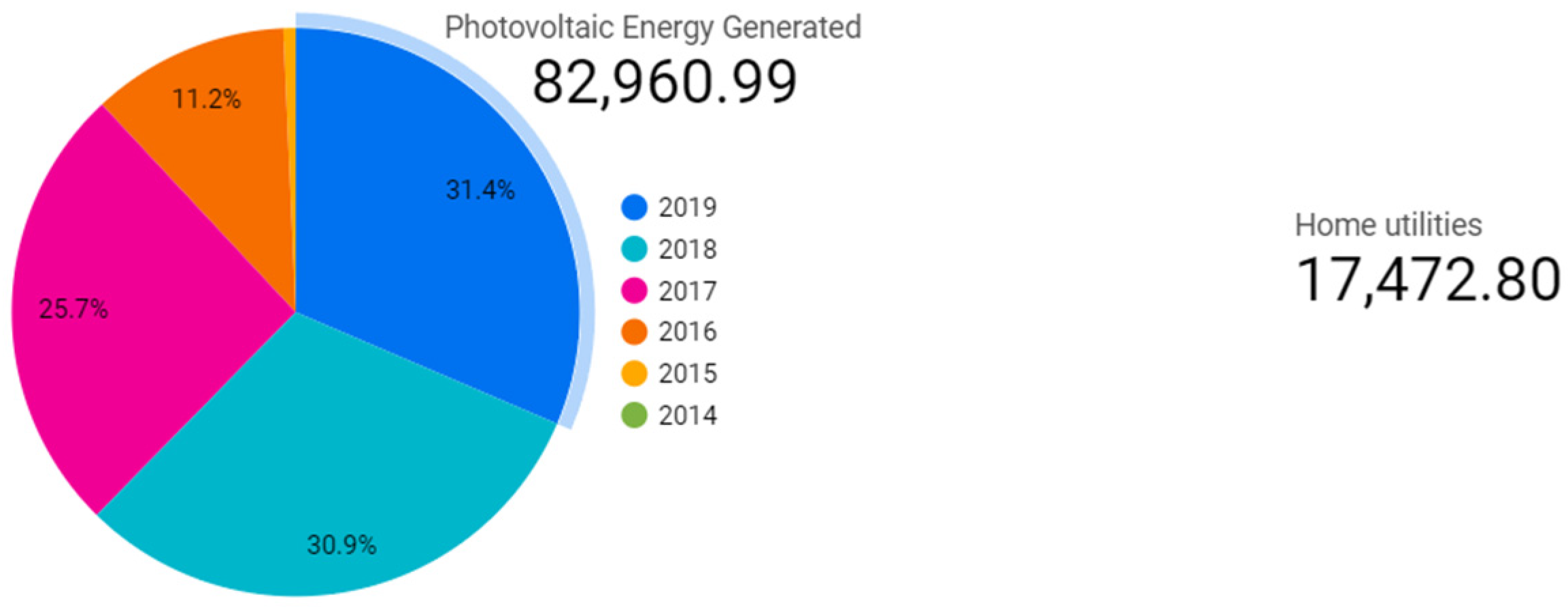
The “Photovoltaic Energy Generated” graph as shown in Figure 18 shows a dramatic increase in solar energy production, which rises from 2015 to 2019, totaling 82,960.99. Of this, 17,472.80 has been used for residential purposes. In 2019, the share of solar energy generated is 31.4 percent, slightly higher than the 30.9 percent in 2018.
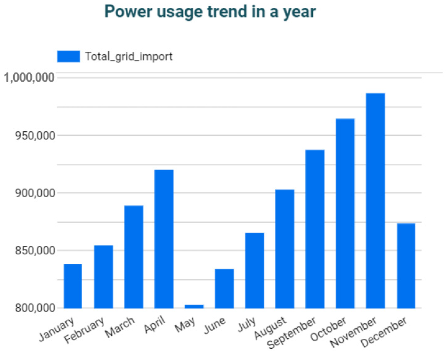
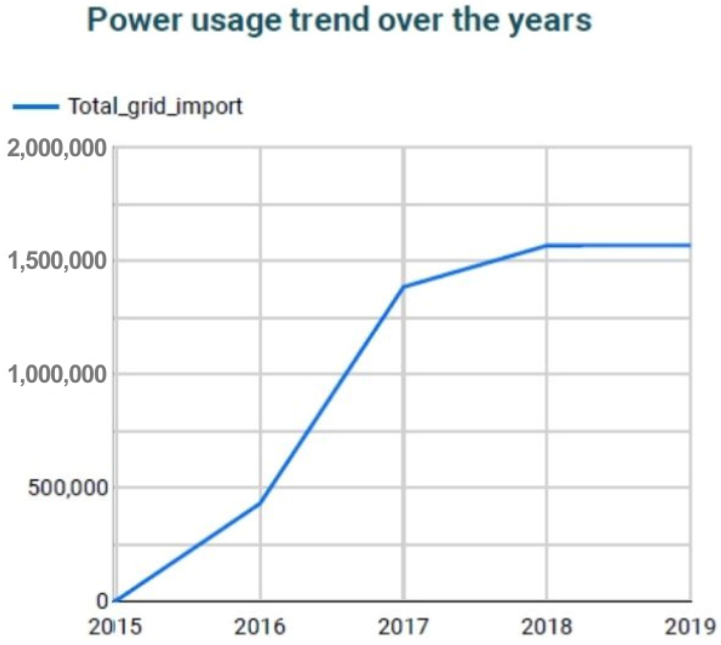
The “Power Usage Trend in a Year” graph as shown in Figure 19 reveals that usage is at its highest from September to November. Meanwhile, the “Power Usage Trend Over the Years” as shown in Figure 20 graph indicates a consistent upward curve from 2015 to 2019. Together, these visualizations offer a multi-dimensional perspective on electricity usage, which is useful for energy analysts and policymakers in understanding and optimizing energy consumption and production.

3.5. Blockchain Integration

Blockchain is a decentralized technology that records transactions across a network of computers, providing a secure and transparent system. For energy grid management, blockchain offers a way to track and verify energy-related transactions without relying on a central authority. This enhances trust among stakeholders, reduces the risk of fraud, and automates various processes through smart contracts. As a result, blockchain can improve the efficiency, reliability, and accountability in managing energy production and distribution.

3.5.1. Software Used

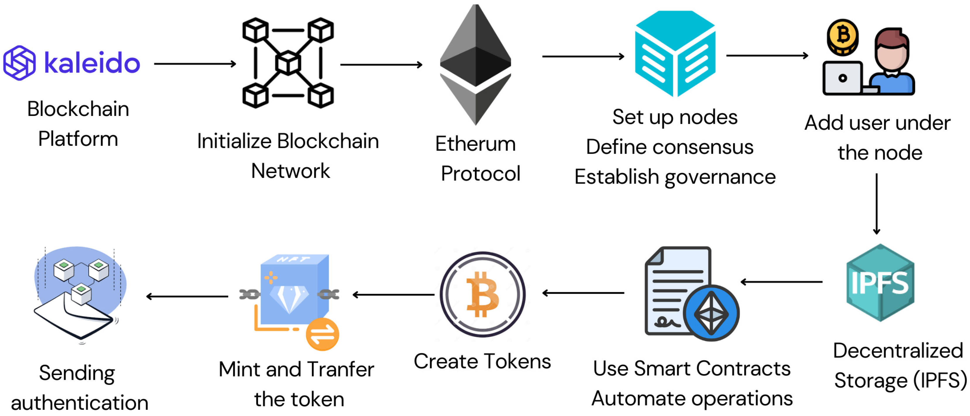
Kaleido is a blockchain-as-a-service platform [34] designed for easy deployment and management of enterprise-grade blockchain networks. Its user-friendly interface allows for the creation of private and consortium networks without needing advanced technical skills. Kaleido supports multiple consensus algorithms, providing flexibility to choose the best method for the needs. With Kaleido, one can deploy blockchain nodes, set up smart contracts [35], and manage network governance in a dedicated sandbox environment. This allows for safe testing and development. A key feature of Kaleido is its integration capabilities, enabling connections with various enterprise tools and services. This makes it easier to link the blockchain network with existing business systems, streamlining operations and improving workflows.
The blockchain network ensures decentralization and data integrity through multiple nodes, each with a complete copy of the blockchain ledger. These nodes validate transactions, achieve consensus, and propagate new blocks. The decentralized structure reduces the risk of fraud and tampering. Consensus mechanisms secure the network by requiring a majority agreement to validate transactions and add new blocks. This approach promotes data integrity and minimizes unauthorized changes. The ability to choose different consensus algorithms also allows for customized security and performance, fostering trust among network participants.
The Hyperledger [36] Firefly framework simplifies deploying and managing blockchain networks. Firefly supernodes act as central hubs, providing an API gateway to integrate with other systems, enabling seamless communication and data exchange. They also manage smart contract deployment and execution, automating processes and reducing intermediaries, thus lowering the risk of errors and fraud. Another key feature of Firefly is its support for tokenization, allowing for the creation of digital tokens to represent assets, rights, or utilities on the blockchain. Tokenization enhances asset tracking, traceability, and flexibility, supporting new business models. Firefly’s tokenization capability streamlines asset management within the blockchain network.
Integrating the IPFS (the Interplanetary File System) into the blockchain network provides decentralized data storage, enhancing resilience and redundancy. IPFS uses content-addressing with unique cryptographic hashes, allowing data to be stored across multiple nodes. This distributed approach offers redundancy, increasing data resilience and reducing the risk of loss due to hardware failures or other disruptions. Including IPFS nodes in the blockchain network ensures that critical data are stored securely, meeting the compliance requirements for data retention and security while improving reliability. This is especially valuable for managing large volumes of data.

3.5.2. Methodology

1.
Start by creating an account on Kaleido’s platform. The full flowchart is explained in Figure 21.
2.
Set Up the blockchain network.
A network was created, with the base region set up using the standard blockchain service, which supports smart contracts and node management. The protocol used was Ethereum, and the consensus algorithm was PoA, thus forming the environment.
3.
Create Memberships
In the Memberships tab, new memberships were created. For this project, memberships were established for “Producer” and “Consumer1.”
4.
Create Firefly Node
To access the Firefly settings, in the Nodes section, add Firefly nodes to manage the smart contracts and facilitate integration. For this project, two Firefly nodes were required, along with corresponding blockchain and IPFS nodes.
5.
Deploy ERC720 Contract
To deploy the ERC720 contract and create and manage the token contracts, we used the FireflyERC720 template and the Token Factory to manage the contract’s deployment.
6.
Teach Firefly About the NFT
Accessing the Firefly tab, using the Web UI of the Consumer node allows interaction with the blockchain network through the Firefly explorer and sandbox. Creating a token pool in the Firefly sandbox initiated the tokenization process.
7.
Mint the NFT
To initiate the minting process within the Firefly sandbox, select the token pool and specify the quantity to mint. Attach a message to the NFT, add additional data, and provide information for the token.
8.
Transfer the NFT and Broadcast a Message
With transfer tokens in the Firefly sandbox, you can initiate a transaction. This can be achieved by selecting the token pool and recipient, transferring the quantity, and adding a message. Then, ensure the tag and topic for traceability, and broadcast a message to the participants about the transaction, thus establishing communication.
9.
Verify That the Producer Has Received the Token
To check the Producer’s node, switch to the producer’s sandbox and Firefly UI to confirm the producer’s interactions. After verifying the token receipt in the Firefly UI and confirming the successful NFT transfer, broadcast a message that the transaction is completed.

3.5.3. Results and Discussions

Kaleido has made setting up the blockchain network straightforward and flexible, with the standard blockchain service and Firefly supernode supporting easy node management as shown in Figure 22. Proof of authority ensured fast validation, while the membership system allowed role-based permissions, creating a secure environment with the producer and consumer roles for the energy grid stakeholders.
The Firefly nodes coordinated the blockchain network and managed smart contracts, facilitating a seamless interaction for the producer and consumer roles. The ERC720 contracts enabled the tokenization of energy assets, while the smart contracts automated processes, reducing intermediaries and errors as shown in Figure 23. Firefly’s tokenization support allowed clear and traceable energy transactions.
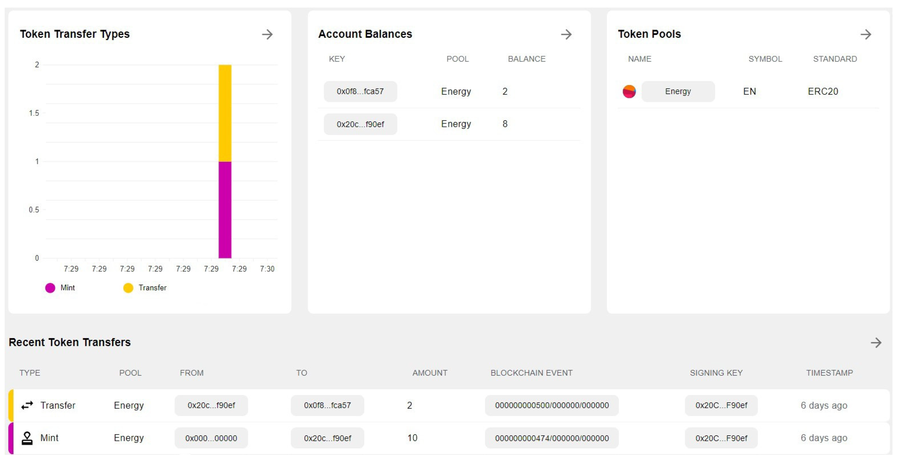
Minting non-fungible tokens (NFTs) using the ERC720 contract demonstrated blockchain’s potential in energy grid management. By creating a token pool and minting NFTs, specific energy units or other assets were represented, enabling efficient asset management and traceability. The ability to transfer NFTs to designated recipients and broadcast messages for context underscored blockchain’s inherent transparency and traceability, allowing enhanced communication among stakeholders as shown in Figure 24.
The final step was to confirm that the producer received the NFT and to broadcast a message to validate the transfer, proving the blockchain network’s successful operation as shown in Figure 25. This step ensured secure and transparent token transfers, with the broadcasted messages providing additional communication and a comprehensive transaction record.
The successful blockchain implementation in energy grid management demonstrated that blockchain technology provided secure, transparent, and traceable transactions, supporting the hypothesis that it could improve security and data integrity. These results suggested that blockchain could reduce the risk of fraud and increase transparency in the energy sector. The use of ERC720 contracts for tokenization opened up new business models, like peer-to-peer energy trading, while the Firefly nodes and smart contracts facilitated automation and enhanced efficiency. Future research could investigate different consensus mechanisms, scalability, and interoperability to ensure that the blockchain networks could adapt to the growing demands of the energy sector.

4. Conclusions

The culmination of this project marks an advancement in revolutionizing energy management frameworks that are universally applicable across different regions and energy systems. By integrating cutting-edge technologies, such as 6G IoT, AI, and blockchain, this study addresses the critical challenges of grid stability, renewable energy integration, and efficient energy management in the context of rapidly increasing global energy demands. As highlighted by the International Energy Agency (IEA), our global energy demand is projected to rise by nearly 50% by 2040, with renewable energy expected to make up about 40% of the global power mix. These trends underscore the urgency of developing robust solutions to manage energy systems more effectively.
The results of this study demonstrate significant improvements in these areas. The stacked ensemble model, which combined SVM, decision tree, and XGBoost, achieved an impressive accuracy of 97.99% in grid-level stability management, outperforming other models in handling complex patterns inherent in the data. In solar energy forecasting, the artificial neural network (ANN) model outperformed others with a root mean squared error (RMSE) of 1.805, indicating superior predictive accuracy. Additionally, reinforcement learning using deep Q networks optimized the microgrid operations, with a clear upward trend in rewards per episode, reflecting the model’s ability to adapt and improve decision-making over time. Furthermore, the introduction of a sophisticated dashboard and blockchain technology has greatly improved transparency and efficiency in energy transactions, highlighting the robustness and scalability of this integrated approach. These findings provide practical solutions for enhancing energy system reliability and sustainability in any region in the world, offering a scalable framework that can be applied to support the integration of renewable energy sources and the development of sustainable smart cities.

5. Additional Explorations

The integration of 6G and optical IoT technologies within smart grid systems offers transformative possibilities that extend beyond our current capabilities. With 6G’s ultra-reliable low-latency communications (URLLC) and optical IoT’s high-bandwidth secure data transmission, the potential for fully autonomous grid management systems becomes increasingly feasible. These systems could dynamically adjust energy distribution and maintenance schedules in real time, leveraging AI-driven predictions to maximize operational efficiency and minimize costs. Additionally, the concept of virtual power plants (VPPs) could be actualized, where diverse renewable energy sources are seamlessly integrated across multiple locations and managed through advanced 6G and optical IoT networks. This would not only optimize energy production based on real-time demands but also substantially enhance the sustainability and resilience of energy networks.
Moreover, the application of these technologies within smart city infrastructures opens up new opportunities for synchronization with other urban utilities, such as water management and transportation systems. The inclusion of state-of-the-art technologies like quantum computing, edge computing, blockchain with smart contracts, digital twins, and Artificial Intelligence of Things (AIoT) further amplifies these advancements. Quantum computing can revolutionize the optimization processes in large-scale grids, while edge computing ensures real-time data processing closer to its source. Blockchain, with smart contracts, can automate and secure energy transactions, and digital twins offer a virtual representation of the grid for real-time monitoring and simulation. The AIoT brings intelligent decision-making directly to edge devices, enabling more autonomous and adaptive grid management. Together, these technologies could revolutionize energy usage patterns, promote greater community engagement in sustainable practices, and significantly contribute to meeting the global sustainability goals while driving future innovation in the energy sector.

Author Contributions

Conceptualization/idea, M.R.A.T.; methodology/software/validation/testing, B.B., M.R.A.T., and S.A.P.R.R.; resources/data curation, M.R.A.T. and B.B.; formal analysis, S.A.P.R.R.; writing-original draft preparation/editing, M.R.A.T., B.B., and S.A.P.R.R.; visualization, B.B.; supervision, R.K.M. and R.C.N.; project administration, R.K.M., P.R., S.R., V.N.K., G.A., and A.M.S. All authors have read and agreed to the published version of the manuscript.

Funding

This research received no external funding.

Data Availability Statement

The datasets used in this study are publicly available and can be accessed through their respective repositories. The Electrical Grid Stability Simulated Dataset [17,18], which was utilized for grid-level stability management research involving artificial neural networks (ANN) and stack ensemble models, is available online. For the Solar Energy Forecasting study, daily and hourly datasets were employed from [25]. These datasets are essential for training and evaluating random forest, ANN, and long short-term memory (LSTM) models and can also be accessed through public repositories. The Microgrid Energy Management research utilized the opsd-household_data-2020-04-15 [31] dataset, which supports the reinforcement learning approaches applied in this study. All datasets mentioned are freely available upon request or can be directly accessed through the provided online repositories.

Conflicts of Interest

All authors declare that they have no conflict of interest.

References

  1. Salam, S.S.A.; Petra, M.I.; Azad, A.K.; Sulthan, S.M.; Raj, V. A Comparative Study on Forecasting Solar Photovoltaic Power Generation Using Artificial Neural Networks. In Proceedings of the 2023 Innovations in Power and Advanced Computing Technologies (i-PACT), Kuala Lumpur, Malaysia, 8–10 December 2023; pp. 1–6. [Google Scholar]
  2. Massaoudi, M.; Abu-Rub, H.; Refaat, S.S.; Chihi, I.; Oueslati, F.S. Accurate Smart-Grid Stability Forecasting Based on Deep Learning: Point and Interval Estimation Method. In Proceedings of the 2021 IEEE Kansas Power and Energy Conference (KPEC), Manhattan, KS, USA, 19–20 April 2021; pp. 1–6. [Google Scholar]
  3. Salam, A.; El Hibaoui, A. Applying Deep Learning Model to Predict Smart Grid Stability. In Proceedings of the 2021 9th International Renewable and Sustainable Energy Conference (IRSEC), Tetouan, Morocco, 23–27 November 2021; pp. 1–9. [Google Scholar]
  4. Abbass, M.J.; Lis, R.; Mushtaq, Z. Artificial Neural Network (ANN)-Based Voltage Stability Prediction of Test Microgrid Grid. IEEE Access 2023, 11, 58994–59001. [Google Scholar] [CrossRef]
  5. Boucetta, L.N.; Amrane, Y.; Arezki, S. Comparative Analysis of LSTM, GRU, and MLP Neural Networks for Short-Term Solar Power Forecasting. In Proceedings of the 2023 (ICEEAT), Batna, Algeria, 19–20 December 2023; pp. 1–6. [Google Scholar]
  6. Singh, A.; Singh, P.; Agrawal, N.; Gupta, P. Estimating the Stability of Smart Grids Using Optimised Artificial Neural Network. In Proceedings of the 2023 International Conference on (REEDCON), New Delhi, India, 1–3 May 2023; pp. 380–384. [Google Scholar]
  7. Redan, R.N.; Othman, M.M.; Hasan, K.; Ahmadipour, M. Random Forest with Daubechies Wavelet and Multiple Time Lags for Solar Irradiance Forecasting. In Proceedings of the 2023 IEEE 3rd (ICPEA), Putrajaya, Malaysia, 6–7 March 2023; pp. 374–378. [Google Scholar]
  8. Foruzan, E.; Soh, L.-K.; Asgarpoor, S. Reinforcement Learning Approach for Optimal Distributed Energy Management in a Microgrid. IEEE Trans. Power Syst. 2018, 33, 5749–5758. [Google Scholar] [CrossRef]
  9. Zhong, Y.-J.; Wu, Y.-K. Short-Term Solar Power Forecasts Considering Various Weather Variables. In Proceedings of the 2020 International Symposium on Computer, Consumer and Control (IS3C), Taichung City, Taiwan, 13–16 November 2020; pp. 432–435. [Google Scholar]
  10. Siriwardana, S.; Nishshanka, T.; Peiris, A.; Boralessa, M.A.K.S.; Hemapala, K.T.M.U.; Saravanan, V. Solar Photovoltaic Energy Forecasting Using Improved Ensemble Method For Micro-grid Energy Management. In Proceedings of the 2022 IEEE 2nd International Symposium on Sustainable Energy, Signal Processing and Cyber Security (iSSSC), Gunupur, Odisha, India, 15–17 December 2022; pp. 1–6. [Google Scholar]
  11. Boumaiza, A.; Sanfilippo, A. AI for Energy: A Blockchain-based Trading market. In Proceedings of the IECON 2022—48th Annual Conference of the IEEE Industrial Electronics Society, Brussels, Belgium, 18–21 October 2022; pp. 1–6. [Google Scholar] [CrossRef]
  12. Sang, Y.; Cali, U.; Kuzlu, M.; Pipattanasomporn, M.; Lima, C.; Chen, S. IEEE SA Blockchain in Energy Standardization Framework: Grid and Prosumer Use Cases. In Proceedings of the 2020 IEEE Power & Energy Society General Meeting (PESGM), Montreal, QC, Canada, 2–6 August 2020; pp. 1–5. [Google Scholar] [CrossRef]
  13. Plaza, C.; Gil, J.; de Chezelles, F.; Strang, K.A. Distributed Solar Self-Consumption and Blockchain Solar Energy Exchanges on the Public Grid Within an Energy Community. In Proceedings of the 2018 IEEE International Conference on Environment and Electrical Engineering and 2018 IEEE Industrial and Commercial Power Systems Europe (EEEIC/I&CPS Europe), Palermo, Italy, 12–15 June 2018; pp. 1–4. [Google Scholar] [CrossRef]
  14. Dimobi, I.; Pipattanasomporn, M.; Rahman, S. A Transactive Grid with Microgrids Using Blockchain for the Energy Internet. In Proceedings of the 2020 IEEE Power & Energy Society Innovative Smart Grid Technologies Conference (ISGT), Washington, DC, USA, 17–20 February 2020; pp. 1–5. [Google Scholar] [CrossRef]
  15. Tiwari, H.; Raj, A.; Singh, U.K.; Fatima, H. Generative AI for NFTs using GANs. In Proceedings of the 2024 11th International Conference on Computing for Sustainable Global Development (INDIACom), New Delhi, India, 28 February–1 March 2024; pp. 488–492. [Google Scholar] [CrossRef]
  16. Hopfield, J.J. Artificial neural networks. IEEE Circuits Devices Mag. 1998, 4, 3–10. [Google Scholar] [CrossRef]
  17. Schäfer, B.; Grabow, C.; Auer, S.; Kurths, J.; Witthaut, D.; Timme, M. Taming instabilities in power grid networks by decentralized control. Eur. Phys. J. Spec. Top. 2016, 225, 569–582. [Google Scholar] [CrossRef]
  18. Arzamasov, V.; Böhm, K.; Jochem, P. Towards Concise Models of Grid Stability. In Proceedings of the 2018 IEEE International Conference on Communications, Control, and Computing Technologies for Smart Grids (SmartGridComm), Aalborg, Denmark, 29–31 October 2018; pp. 1–6. [Google Scholar]
  19. Ho, T.K. The random subspace method for constructing decision forests. IEEE Trans. Pattern Anal. Mach. Intell. 1998, 20, 832–844. [Google Scholar] [CrossRef]
  20. Hearst, M.A.; Dumais, S.T.; Osuna, E.; Platt, J.; Scholkopf, B. Support vector machines. IEEE Intell. Syst. Their Appl. 1998, 13, 18–28. [Google Scholar] [CrossRef]
  21. Chen, T.; Guestrin, C. XGBoost: A Scalable Tree Boosting System. In Proceedings of the 22nd ACM SIGKDD International Conference on Knowledge Discovery and Data Mining (KDD ‘16), San Francisco, CA, USA, 13–17 August 2016; Association for Computing Machinery: New York, NY, USA, 2016; pp. 785–794. [Google Scholar] [CrossRef]
  22. Shahriari, B.; Swersky, K.; Wang, Z.; Adams, R.P.; de Freitas, N. Taking the Human Out of the Loop: A Review of Bayesian Optimization. Proc. IEEE 2015, 104, 148–175. [Google Scholar] [CrossRef]
  23. Bergstra, J.; Bengio, Y. Random Search for Hyper-Parameter Optimization. J. Mach. Learn. Res. 2012, 13, 281–305. [Google Scholar]
  24. Rodriguez, J.D.; Perez, A.; Lozano, J.A. Sensitivity Analysis of k-Fold Cross Validation in Prediction Error Estimation. IEEE Trans. Pattern Anal. Mach. Intell. 2010, 32, 569–575. [Google Scholar] [CrossRef] [PubMed]
  25. Available online: https://github.com/ColasGael/Machine-Learning-for-Solar-Energy-Prediction/tree/master/Datasets/ (accessed on 28 January 2024).
  26. Ho, T.K. Random decision forests. In Proceedings of the 3rd International Conference on Document Analysis and Recognition, Montreal, QC, Canada, 14–15 August 1995; Volume 1, pp. 278–282. [Google Scholar] [CrossRef]
  27. Schuster, M.; Paliwal, K.K. Bidirectional recurrent neural networks. IEEE Trans. Signal Process. 1997, 45, 2673–2681. [Google Scholar] [CrossRef]
  28. Graves, A.; Schmidhuber, J. Framewise phoneme classification with bidirectional LSTM networks. In Proceedings of the 2005 IEEE International Joint Conference on Neural Networks, Montreal, QC, Canada, 31 July–4 August 2005; Volume 4, pp. 2047–2052. [Google Scholar] [CrossRef]
  29. Sutton, R.S.; Barto, A.G.; Learning, R. Reinforcement Learning: An Introduction. IEEE Trans. Neural Netw. 1998, 9, 1054. [Google Scholar] [CrossRef]
  30. Microgrid Controllers: Functions and Benefits. Available online: https://247mesa.com/microgrid-controllers-functions-and-benefits/ (accessed on 12 December 2023).
  31. Open Power System Data. 2020. Data Package Household Data. Version 15 April 2020. Available online: https://data.open-power-system-data.org/household_data/2020-04-15/ (accessed on 10 January 2024).
  32. Gupta; Goswami, P.; Chaudhary, N.; Bansal, R. Deploying an Application using Google Cloud Platform. In Proceedings of the 2020 2nd International Conference on Innovative Mechanisms for Industry Applications (ICIMIA), Bangalore, India, 5–7 March 2020; pp. 236–239. [Google Scholar] [CrossRef]
  33. Pulipati, S. Data Storytelling with Google Looker Studio: A Hands-on Guide to Using Looker Studio for Building Compelling and Effective Dashboards; Packt Publishing: Birmingham, UK, 2022. [Google Scholar]
  34. Samaniego, M.; Jamsrandorj, U.; Deters, R. Blockchain as a Service for IoT. In Proceedings of the 2016 IEEE International Conference on Internet of Things (iThings) and IEEE Green Computing and Communications (GreenCom) and IEEE Cyber, Physical and Social Computing (CPSCom) and IEEE Smart Data (SmartData), Chengdu, China, 15–18 December 2016; pp. 433–436. [Google Scholar] [CrossRef]
  35. Christidis, K.; Devetsikiotis, M. Blockchains and Smart Contracts for the Internet of Things. IEEE Access 2016, 4, 2292–2303. [Google Scholar] [CrossRef]
  36. Thakkar, P.; Nathan, S.; Viswanathan, B. Performance Benchmarking and Optimizing Hyperledger Fabric Blockchain Platform. In Proceedings of the 2018 IEEE 26th International Symposium on Modeling, Analysis, and Simulation of Computer and Telecommunication Systems (MASCOTS), Milwaukee, WI, USA, 25–28 September 2018; pp. 264–276. [Google Scholar] [CrossRef]
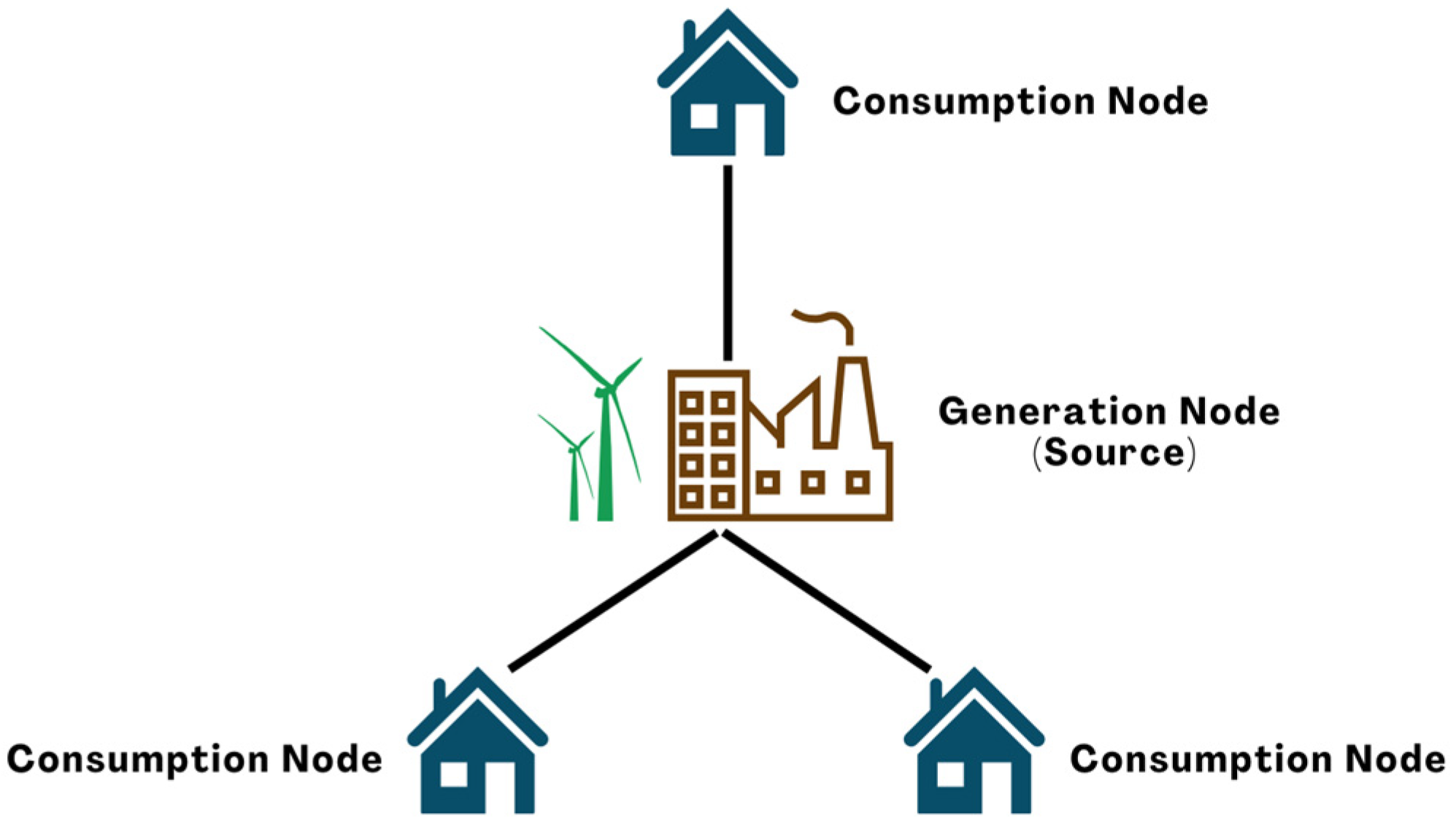
Figure 1. 4 Node star network.
Iot 05 00025 g001
Figure 2. Flowchart of grid-level management.
Iot 05 00025 g002
Figure 3. Stacked ensemble receiver operating characteristic.
Iot 05 00025 g003
Figure 4. Stacked ensemble confusion matrix.
Iot 05 00025 g004
Figure 5. ANN receiver operating characteristic.
Iot 05 00025 g005
Figure 6. ANN confusion matrix.
Iot 05 00025 g006
Figure 7. Workflow diagram of solar energy.
Iot 05 00025 g007
Figure 8. Flowchart of solar energy forecasting.
Iot 05 00025 g008
Figure 9. Prediction by random forest.
Iot 05 00025 g009
Figure 10. Prediction by artificial neural network.
Iot 05 00025 g010
Figure 11. Prediction by LSTM.
Iot 05 00025 g011
Figure 12. Workflow diagram of reinforcement learning [30].
Iot 05 00025 g012
Figure 13. Flowchart of microgrid management.
Iot 05 00025 g013
Figure 14. Total rewards per episode.
Iot 05 00025 g014
Figure 15. Loss over training steps over 40 episodes.
Iot 05 00025 g015
Figure 16. Flowchart of interactive data visualization.
Iot 05 00025 g016
Figure 17. Grid energy import and usage pattern.
Iot 05 00025 g017
Figure 18. The photovoltaic energy generated.
Iot 05 00025 g018
Figure 19. Power usage trend in a year.
Iot 05 00025 g019
Figure 20. Power usage trends over the years.
Iot 05 00025 g020
Figure 21. Workflow of a blockchain transaction.
Iot 05 00025 g021
Figure 22. Blockchain network setup.
Iot 05 00025 g022
Figure 23. Firefly node setup and tokenization.
Iot 05 00025 g023
Figure 24. Minting and transferring tokens.
Iot 05 00025 g024
Figure 25. Dashboard of token transfer.
Iot 05 00025 g025
Table 1. Stacked ensemble classification report.
PrecisionRecallF1-ScoreSupport
Stable0.970.970.974322
Unstable0.980.990.987678
Accuracy 0.9812,000
Macro Avg0.980.980.9812,000
Weighted Avg0.980.980.9812,000
Table 2. ANN with Bayesian optimization classification report.
PrecisionRecallF1-ScoreSupport
Stable0.960.970.974322
Unstable0.980.980.987678
Accuracy 0.9812,000
Macro Avg0.970.980.9712,000
Weighted Avg0.980.980.9812,000
Table 3. Solar power generation data.
ColumnDescription
DATE_TIME15 min timestamp
PLANT_IDConstant value throughout
SOURCE_KEYUnique inverter ID
DC_POWERDC power generated by that inverter
AC_POWERAC power after conversion
DAILY_YIELDTotal power generated that day
TOTAL_YIELDTotal inverter yield
Table 4. Weather sensor data.
ColumnDescription
DATE_TIME15 min timestamp
PLANT_IDConstant value throughout
SOURCE_KEYUnique inverter ID
AMBIENT_TEMPERATUREAmbient temperature at the plant
MODULE_TEMPERATURE AC power after conversion
IRRADIATIONAmount of irradiation
Table 5. Comparison of solar forecasting models with RMSE.
S. No.Model UsedRMSE Error
1Random forest1.908
2Artificial neural network1.805
3Bidirectional LSTM2.055
Table 6. Deviation of actual energy and predicted energy for 3 days.
DateHourActual Gen (MW)Predicted Gen (MW)Deviation %
15-06-2020813.22912.257−7.349
99.74510.5868.635
1011.34810.965−3.376
118.9988.732−2.953
129.9779.366−6.121
138.9527.413−17.198
1410.98010.634−3.150
159.64310.1194.930
168.0176.966−13.115
173.4065.64565.754
182.0542.68830.837
16-06-202089.92710.2843.601
911.90610.767−9.564
1015.52713.166−15.205
1116.45614.503−11.869
1215.37813.143−14.532
1315.83114.591−7.834
147.9709.66221.224
1512.19511.304−7.306
165.6297.49733.170
171.9942.63031.898
180.8352.203163.803
17-06-202084.6655.98528.285
97.2477.6084.980
1010.85811.7428.141
1112.2499.925−18.971
1215.44113.208−14.460
1312.07114.02216.161
1410.76810.040−6.759
1510.15410.4232.645
165.8406.4179.888
172.3213.56753.689
181.3262.951122.454
Table 7. Two solar power plants’ generation.
ColumnDescription
utc_timestamp15 min timestamp
grid_importUnits used from grid
pvSolar energy produced
storage_chargeUnits charged
storage_dechargeUnits discharged
Disclaimer/Publisher’s Note: The statements, opinions and data contained in all publications are solely those of the individual author(s) and contributor(s) and not of MDPI and/or the editor(s). MDPI and/or the editor(s) disclaim responsibility for any injury to people or property resulting from any ideas, methods, instructions or products referred to in the content.