Efficient Sensing Data Collection with Diverse Age of Information in UAV-Assisted System

Abstract

With the high flexibility and low cost of the deployment of UAVs, the application of UAV-assisted data collection has become widespread in the Internet of Things (IoT) systems. Meanwhile, the age of information (AoI) has been adopted as a key metric to evaluate the quality of the collected data. Most of the literature generally focuses on minimizing the age of all information. However, minimizing the overall AoI may lead to high costs and massive energy consumption. In addition, not all types of data need to be updated highly frequently. In this paper, we consider both the diversity of different tasks in terms of the data update period and the AoI of the collected sensing information. An efficient data collection method is proposed to maximize the system utility while ensuring the freshness of the collected information relative to their respective update periods. This problem is NP-hard. With the decomposition, we optimize the upload strategy of sensor nodes at each time slot, as well as the hovering positions and flight speeds of UAVs. Simulation results show that our method ensures the relative freshness of all information and reduces the time-averaged AoI by $96.5\%$, $44\%$, $90.4\%$, and $26\%$ when the number of UAVs is 1 compared to the corresponding EMA, AOA, DROA, and DRL-eFresh, respectively.

1. Introduction

1.1. Growing Volume of Data Generated by IoT

As indicated by Forbes, in light of the exponential expansion of the Internet of Things (IoT) and the surge of big data, it is projected that the volume of generated data will reach an astounding 175 ZB by the year 2025 [1]. This will create enormous opportunities and challenges for applications in various technical fields, such as smart cities, smart transportation, smart grids, natural disaster monitoring, etc. Various data collection methods have been proposed to realize effective data collection to cope with the increasing amount of information.

1.2. Role of UAVs in Data Collection

UAVs have gained significant attention and found numerous applications in data collection and network coverage expansion because of simple deployment, high mobility, and low operating costs. UAVs collect data from various locations and transmit them to the base station (BS) for further processing. Wireless sensor nodes provide timely sensing data for various applications, including search-and-rescue operations, emergency response, and disaster monitoring. The fully controllable maneuverability of UAVs allows them to approach ground equipment and establish a low air-to-ground communication link. In the case of a limited ground Internet infrastructure, UAVs can flexibly collect sensing data from sensor nodes deployed on the ground, save the transmission energy of sensor nodes, and prolong the lifetime of sensor networks. Integrating UAVs into communication networks presents a series of challenging design issues, such as UAV functionality, flight trajectory design, and energy efficiency.

UAVs could act as mobile stations [2] or flying relays [3], providing reliable communication with small and power-limited terrestrial wireless devices. UAVs could also be used as mobile edge computing (MEC) servers [4], transforming them into an effective means of data collection and auxiliary computing. This could reduce the power consumption and computing burden of IoT devices.

1.3. Importance of Energy Efficiency

Liu et al. in [5] proposed an iterative sensor node association and trajectory planning strategy for UAVs. Optimizing the trajectory and speed of the UAV can enhance system performance [6,7,8]. In [9,10], all the authors studied the development of optimal UAV flight trajectories based on energy-efficient strategies. Optimizing the flight trajectories of UAVs can achieve the minimum energy consumption, depending on the flight speed, direction, and acceleration of UAVs.

The size and weight of UAVs are limited, and their onboard energy constrains their performance and range. The energy efficiency of UAV-assisted systems is one of the most important research topics. Zeng et al. in [10] proposed an efficient design to maximize energy efficiency under the constraints of minimum and maximum velocity and acceleration of the UAV. Ahmed et al. in [11] maximized the throughput by optimizing the trajectory and transmission power of the UAV. In [10,12], the authors considered both the communication throughput and energy consumption of UAVs and proposed efficient designs to optimize the behavior of UAVs, including speed and hovering position. Samir et al. in [7] transformed the energy efficiency problem into maximizing the throughput to energy consumption ratio and addressed the component problem with the Dinkelbach method.

1.4. Freshness of Information

The studies mentioned above meticulously investigated the trajectory optimization of the UAV and the improvement of the energy efficiency of the system. UAVs enhance the effectiveness of data collection in IoT systems. Furthermore, there is currently a significant focus on information freshness in the research community.

The age of information (AoI) has been used as a performance metric to evaluate the freshness of collected data. AoI measures the elapsed time since the generation of the last received update. Unlike throughput or latency, which are packet-centric measures, AoI focuses on the destination node and is better suited for assessing the timeliness of updates. The vast majority of studies concentrate on obtaining fresh data. In [2,4,5,13,14,15,16], the authors aimed to minimize the average AoI of all tasks to achieve the freshness of the entire system. In [3,5,12], the authors attempted to estimate the freshness of information by the concept of peak AoI, as it provides the peak value of the AoI. On the other hand, in [6,7], the authors focused on the age of overall information.

1.5. Contribution of Our Work

The studies above did not consider the diverse AoI requirements of different tasks. In particular, users have varying needs across different applications. In some IoT applications, the status of the sensing target changes rapidly, requiring a high frequency of data collection and transmission to keep the sensing data up to date. For instance, road traffic monitoring requires real-time data, updated once every minute, while environmental monitoring data can be updated less frequently, such as once every hour. Therefore, it is not necessary to equally reduce the AoI for all tasks. The focus should be on considering the relative freshness of information to meet the update requirements of different tasks. Given the diverse AoI requirements of different tasks, optimizing the UAVs’ trajectory and flight speed becomes crucial to ensure the relative freshness of information for each task. Moreover, the flight speed of the UAV is directly linked to energy consumption, making it essential to strike a balance between maximizing system utility, minimizing energy consumption, and maintaining the relative freshness of information for various tasks. Achieving this delicate balance presents a significant challenge.

In this paper, we jointly consider the diverse needs of different tasks for the update period and the maximization of the amount of data collected by UAVs with the lowest energy consumption. The main contributions of this paper are as follows:

• We propose an efficient data collection method to ensure the relative freshness of the sensing data of different tasks rather than blindly minimizing the age of all information. We consider the data collection for tasks with different update requirements. Not all types of data require high-frequency updates.
• We propose an algorithm to maximize the system utility. The flight speeds and flight trajectories of the UAVs at each time slot are optimized. UAVs consume energy during the movement stage, the data collection stage, and the data transmission stage. Throughout the process, the objective is to collect more data while minimizing energy consumption and maintaining the relative freshness of different types of information.
• Our proposed method outperforms the other four methods in terms of average AoI. Specifically, the proposed method can reduce the time-averaged AoI by $96.5\%$, $44\%$, $90.4\%$, and $26\%$ compared with the counterparts EMA, AOA, DROA, and DRL-eFresh, respectively, when the number of UAVs is 1. In addition, our proposed method can achieve the relative freshness of information for the collected sensing data with different update periods.

The remainder of this paper is organized as follows. Section 2 summarizes the related works. The system model is described in Section 3. We introduce the problem formulation and propose the iterative optimization algorithm in Section 4. We then discuss the performance evaluation in Section 5. Finally, the conclusions of the paper are in Section 6.

2. Related Works

This section presents the related works, which consist of UAV-aided communication and the AoI in IoT systems.

Table 1. Comparison of our method with other state-of-the-art approaches.

Year	Reference	Main Focus	Energy Efficiency	Trajectory Design	Security	UAV-Swarm	AoI
2023	Proposed work	Diverse AoI requirements	√	√		√	√
2023	[9]	Delay-sensitive, geographical fairness	√	√		√
2023	[17]	Energy recharging	√	√			√
2023	[15]	Total average AoI		√		√	√
2022	[18]	Real-time trajectory plan	√	√		√
2022	[19]	Security challenges			√
2022	[20]	UAV swarm control				√

depicts the comparison of the current work with other state-of-the-art approaches.

In recent years, there has been a growing interest in leveraging UAVs as an auxiliary method for data collection within the IoT domain. Some articles focus on data transmission in communication. Refs. [3,7] proposed UAV-assisted intelligent systems that can collect data packets from vehicles. Refs. [2,5] analyzed the communication between UAVs and ground sensors.

Some studies focused on the energy consumption of UAVs. Zeng et al. in [10] proposed that the propulsion energy consumption of UAVs is determined by their flight speed and acceleration. The authors maximized the data transmission rate while minimizing energy consumption, and energy-efficient systems could be designed. In addition, Yang et al. in [11] considered the energy efficiency of the system and also optimized the flight trajectory of the UAV. The team jointly considered the UAV throughput and propulsion energy consumption. The flight path, transmission power, and flight speed of the UAV were optimized to maximize the throughput. Che et al. in [21] proposed UAV-assisted wireless energy transmission and wireless information transmission modes, where the UAV transmitted wireless information and energy to a low-power terminal. The authors in [18] proposed a continuous and real-time path planning model and a task allocation model, where heterogeneous teams of UAVs from different BSs are used to collect readings from ground sensors and pass these readings to ground sensors.

UAVs are highly susceptible to cyberattacks due to their open operational characteristics, leading to significant security vulnerabilities, including cyberattacks and eavesdropping on navigation and communication links. Considering the widespread use of UAVs, the demands for UAV communication security escalated significantly. Military UAVs are relatively secure, and in [22], the authors proposed a secure UAV communication system specifically designed for military environments. This system ensures perfect forward secrecy, maintains secure UAV-to-UAV (and UAV-to-global control system) communications, and supports non-repudiation. However, all other UAVs are vulnerable to being hijacked or misused, similar to any other connected device. In [19], the focus was on the security challenges related to UAV usage. They aimed to identify the primary types of security attacks that might target UAVs and explored various countermeasures that could be implemented to address these threats and attacks effectively. The authors in [23] addressed the issue of secure communication between UAVs and multiple ground users. They proposed a Q-learning-based approach aimed at maximizing the average secrecy rate (ASR) and enhancing the overall security of the communication system.

When UAVs operate with a certain level of autonomy, the careful planning of task execution and resource optimization becomes crucial to achieve specific objectives. In [20], the authors proposed a UAV swarm communication model for search and rescue applications, utilizing machine learning methods. They analyzed a dataset comprising five triangular swarm formations using the K-means clustering method and studied dendrograms to identify correct swarm formations. In [24], a UAV swarm model was developed with a multilevel-based clustering approach. The authors proposed a tree-based multi-stage scheme employing clustering localization and designed a localization algorithm using a coalitional game framework to explore the model’s features. In [25], the authors enhanced the multi-UAV collaborative tasking algorithm by incorporating fuzzy mean (FCM) clustering and ant colony optimization (ACO) algorithm concepts. Qu et al. in [26] investigated the challenge of efficient edge intelligence (e-EIC) within a UAV swarm network clustering context. They focused on jointly optimizing computation resource allocation and UAV clustering to minimize the total energy consumption of the UAV swarm.

AoI is considered a key performance metric in UAV-assisted IoT systems. Dai et al. in [9] jointly considered the amount of collected data, geographic fairness, and energy consumption and utilized data durability to ensure its freshness. In [2], Dai et al. proposed using MU-MIMO techniques between UAVs and sensor nodes to collect data and minimize the average AoI, characterizing the freshness of the system.

Furthermore, both [2,9] focused on optimizing the overall AoI of the system. Zhang et al. in [6] considered the sensing time, transmission time, and UAV path optimization to minimize the total AoI of the tasks. Liu et al. in [5] defined the sum of data upload time and UAV flight time for all sensor nodes as AoI and optimized both the peak and average AoI.

However, little research has considered the relative freshness of information from tasks with diverse update periods. We need to consider not only the diverse needs of different tasks and the optimization of the flight trajectories and flight speeds of UAVs. In addition, we need to achieve a trade-off between the energy consumption and the AoI of tasks.

3. System Model

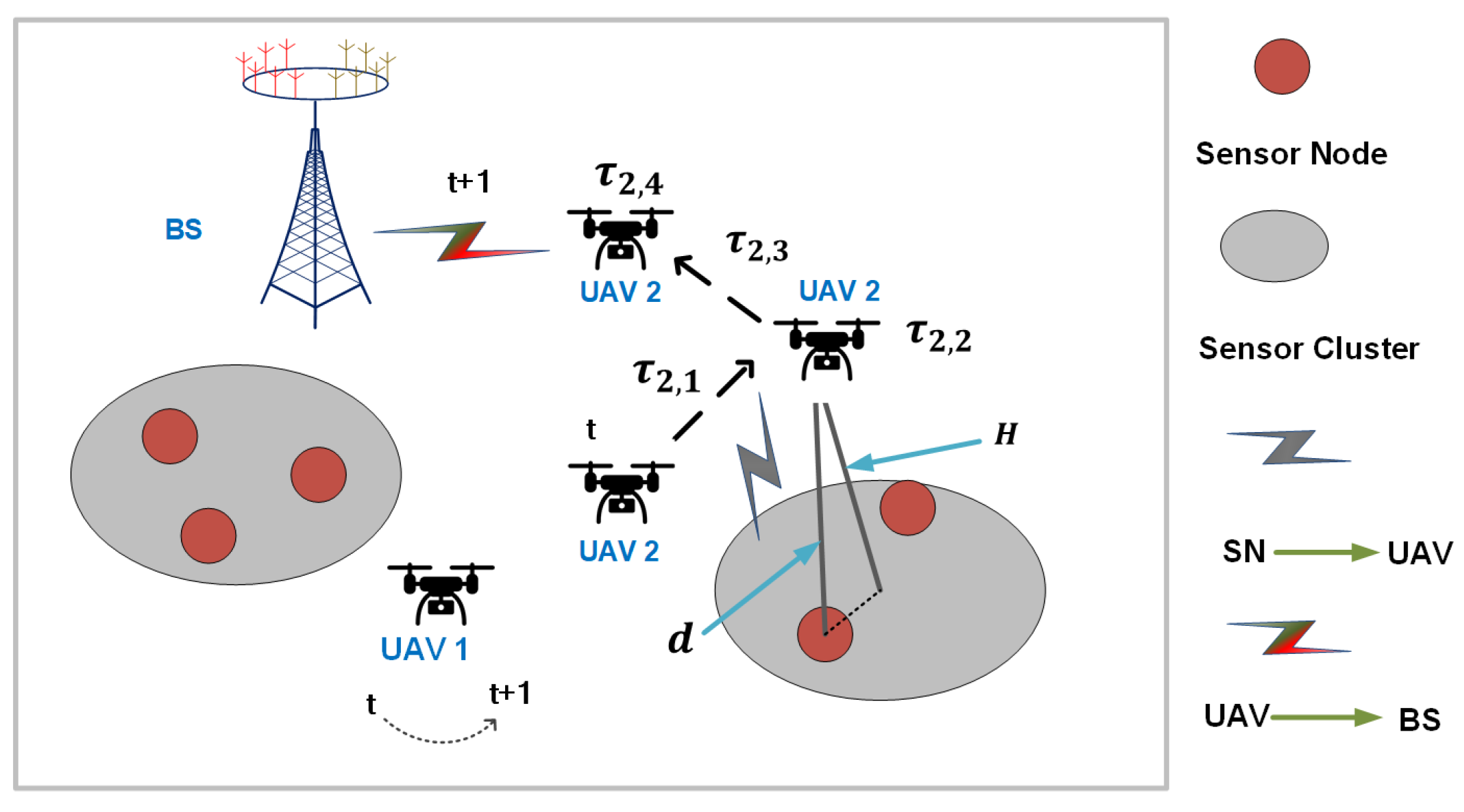
As shown in Figure 1, we consider a UAV-assisted sensing data collection system consisting of one BS, several UAVs, and multiple sensor nodes. Let $\mathcal{N}=\{1,2,\dots ,N\}$ and $\mathcal{M}=\{1,2,\dots ,M\}$ denote the set of UAVs and sensor nodes, respectively. UAVs are scheduled to collect data from sensor nodes and transmit the collected data back to the BS. The location of each sensor node $j\in \mathcal{M}$ and the BS is represented by three coordinates as $l_j^{sn}=(x_j^{sn},y_j^{sn},0)$ and $l^{bs}=(x^{bs},y^{bs},H^{bs})$, respectively. We consider a time-slotted system with $\mathcal{T}=\{1,2,\dots ,T\}$, and the time duration of each time slot is denoted as $t_f$.

We assume that UAVs fly at a fixed altitude H. Then, the UAV trajectory can be considered two-dimensional movement on the horizontal plane. At each time slot t, UAV $i\in \mathcal{N}$ has two stop locations denoted as $l_{i,1}^{uav}(t)=(x_{i,1}^{uav}(t),y_{i,1}^{uav}(t),H)$ and $l_{i,2}^{uav}(t)=(x_{i,2}^{uav}(t),y_{i,2}^{uav}(t),H)$, respectively. At the first stop location $l_{i,1}^{uav}(t)$, UAV i is arranged to collect data from sensor nodes. At the second stop location $l_{i,2}^{uav}(t)$, UAV i transmits the collected data to the BS.

3.1. Channel Models

Channel model between UAV and sensor node: We consider both line-of-sight (LoS) and non-line-of-sight (NLoS) channels between UAVs and sensor nodes. According to the channel modeling in [27], the probability that there exists LoS and NLoS link between UAV i and sensor node j can be expressed as

$$p_{i,los}^j={(1+aexp(-b[\frac{180}{\pi }arcsin(\frac{H}{d_i^j(t)})-a]))}^{-1}$$

(1)

and

$$p_{i,nlos}^j=1-p_{i,los}^j,$$

(2)

respectively, where a and b are environment parameters. $d_i^j(t)$ is the distance between UAV i and sensor node j, which can be expressed as

$$d_i^j(t)=\parallel l_{i,1}^{uav}(t)-l_j^{sn}\parallel .$$

(3)

The channel gain for the communication channel between UAV i and sensor node j can be given as [27]

$$h_i^j(t)=\frac{{\beta }_0}{{(\frac{4\pi f_c}{c})}^2{(d_i^j(t))}^2[p_{i,los}^j{\mu }_{los}+p_{i,nlos}^j{\mu }_{nlos}]},$$

(4)

where $f_c$ is the UAVs carrier frequency, and c is the speed of light. ${\mu }_{los}$ and ${\mu }_{nlos}$ are average additional losses to free space propagation for LoS and NLoS connections, which depend on the environment. ${\beta }_0$ is the channel gain at the reference distance $d_0=1$ m. The data transmission rate of sensor node j to UAV i is expressed as [28]

$$R_i^j(t)=B_i{log}_2[1+\frac{P_j(t)h_i^j(t)}{{\sigma }^2}],$$

(5)

where $B_i$ is the bandwidth allocated to UAV i, and ${\sigma }^2$ denotes the noise power. $P_j(t)$ is the transmission power of sensor node j.

Channel model between UAV and BS: We consider LoS channels between UAVs and the BS. Therefore, the channel gain between UAV i and the BS can be expressed as follows [27]:

$$h_{uav,i}^{bs}(t)=\frac{{\beta }_0}{{(\frac{4\pi f_c}{c})}^2{(d_{uav,i}^{bs}(t))}^2},$$

(6)

where $d_{uav,i}^{bs}(t)$ is the distance between UAV i and the BS, $d_{uav,i}^{bs}(t)=\parallel l_{i,2}^{uav}(t)-l^{bs}\parallel$. Therefore, the data transmission rate can be expressed as [28]

$$R_{uav,i}^{bs}(t)=B_i{log}_2[1+\frac{P_i(t)h_{uav,i}^{bs}(t)}{{\sigma }^2}],$$

(7)

where UAV i transmits data and reuses bandwidth $B_i$. $P_i(t)$ is the transmission power of UAV i.

3.2. UAVs’ Behavior and Features

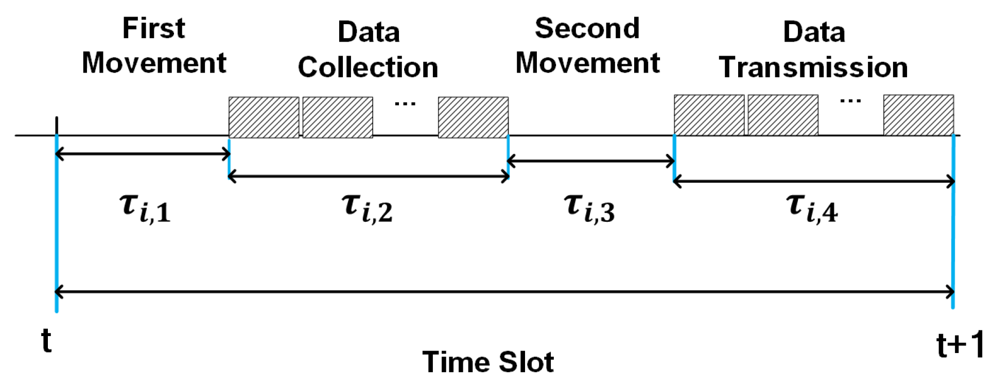
At each time slot, UAV i firstly moves to the first stop location to collect data from sensing nodes within its coverage. Then, with the collected sensing data, UAV i moves to the second stop location and transmits the collected sensing data to the BS. Therefore, we divide the behavior of UAV i at each time slot into four stages as shown in Figure 2: the first movement stage, the data collection stage, the second movement stage, and the data transmission stage.

The energy consumption of UAV i consists of three parts: (1) propulsion energy during two movement stages denoted as $E_{i,1}(t)$ and $E_{i,3}(t)$ respectively; (2) hovering energy during the data collection stage denoted as $E_{i,2}(t)$; and (3) transmission energy during the data transmission stage denoted as $E_{i,4}(t)$. The corresponding energy consumption of UAV i at each stage is elaborated in detail as follows.

• The first movement stage: Given that UAV i will fly to the first stop location $l_{i,1}^{uav}(t)$ with a constant speed $v_{i,1}(t)$, the flight distance is $\parallel l_{i,1}^{uav}(t)-l_{i,0}^{uav}(t)\parallel$, where $l_{i,1}^{uav}(t)$ and $l_{i,0}^{uav}(t)$ are the first stop location and initial location of UAV i at time slot t, respectively. So the time duration of the first movement stage is

  $${\tau }_{i,1}(t)=\frac{\parallel l_{i,1}^{uav}(t)-l_{i,0}^{uav}(t)\parallel }{v_{i,1}(t)}.$$

  (8)
  The propulsion energy consumed by UAV i during the first movement stage can be expressed as [29]

  $$\begin{array}{c}\hfill \begin{array}{cc}& \hfill E_{i,1}(t)=[s_1(1+\frac{3{(v_{i,1}(t))}^2}{{(v_{tip})}^2})+s_2{(\sqrt{1+\frac{{(v_{i,1}(t))}^4}{4{(v_0)}^4}}-\frac{{(v_{i,1}(t))}^2}{2{(v_0)}^2})}^{\frac{1}{2}}+\frac{1}{2}{s}_3{(v_{i,1}(t))}^3]·{\tau }_{i,1}(t),\hfill \end{array}\end{array}$$

  (9)

  where $s_1$, $s_2$, $s_3$ are constants corresponding to the blade profile power, derived power, and air resistance, respectively; $v_{tip}$ represents the tip speed of the rotor blade; and $v_0$ is the mean rotor induced velocity in hovering, a constant for each UAV.
• The data collection stage: At this stage, UAV i hovers at the first stop location $l_{i,1}^{uav}(t)$ to collect data from sensor nodes within its coverage. The associated sensor nodes are scheduled to upload their sensed data to the UAV using multiple access schemes. In this paper, we apply the time division multiple access (TDMA) scheme, where each sensor node j performs its current sensing task and packs data into a packet of length $L_j$. The corresponding sensor nodes then sequentially upload data to UAV i. Thus, the data collection time is denoted as

  $${\tau }_{i,2}(t)=\sum _{j\in \mathcal{M}}{\alpha }_j(t)\frac{L_j}{R_i^j(t)},$$

  (10)
  ${\alpha }_j(t)$ is the data uploading decision of sensor node j at time slot t.
  The energy consumption by UAV i when hovering for data collection can be given as follows:

  $$E_{i,2}(t)=P_0\times {\tau }_{i,2}(t),$$

  (11)

  where $P_0$ is the hovering power for each UAV.
• The second movement stage: After all data are uploaded, UAV i will fly to the second stop location $l_{i,2}^{uav}(t)$ with speed $v_{i,2}(t)$. Location $l_{i,2}^{uav}(t)$ is determined by the movement time ${\tau }_{i,3}(t)$ and UAV i’s data transmission rate $R_{uav,i}^{bs}(t)$, which corresponds to the distance between UAV i and the BS. The time it takes for UAV i to perform the second movement is

  $${\tau }_{i,3}(t)=\frac{\parallel l_{i,2}^{uav}(t)-l_{i,1}^{uav}(t)\parallel }{v_{i,2}(t)}.$$

  (12)
  The propulsion energy consumed by UAV i during the second movement stage can be expressed as [29]

  $$\begin{array}{c}\hfill \begin{array}{c}\hfill E_{i,3}(t)=[s_1(1+\frac{3{(v_{i,2}(t))}^2}{{(v_{tip})}^2})+s_2{(\sqrt{1+\frac{{(v_{i,2}(t))}^4}{4{(v_0)}^4}}-\frac{{(v_{i,2}(t))}^2}{2{(v_0)}^2})}^{\frac{1}{2}}+\frac{1}{2}{s}_3{(v_{i,2}(t))}^3]·{\tau }_{i,3}(t).\end{array}\end{array}$$

  (13)
• The data transmission stage: At this stage, the collected data are transmitted to the BS. The data transmission time depends on the amount of data and the second stop location of UAV i. It can be expressed as follows:

  $${\tau }_{i,4}(t)=\sum _{j\in \mathcal{M}}{\alpha }_j(t)\frac{L_j}{R_{uav,i}^{bs}(t)}.$$

  (14)
  The energy consumption by UAV i during the transmission stage can be expressed as

  $$E_{i,4}(t)=P_i(t)\times {\tau }_{i,4}(t).$$

  (15)

In summary, when a UAV $i\in \mathcal{N}$ is arranged to collect data, it either moves or hovers to complete tasks (e.g., data collection or data transmission), consuming different amounts of energy. It is important to note that not all UAVs are assigned to collect sensing data during each time slot. For those UAVs that are not assigned to collect data during a particular time slot (e.g., UAV 1 in Figure 1), they simply keep hovering with an energy consumption of $P_0\times t_f$, where $P_0$ is the hovering power of each UAV, and $t_f$ is the duration of one time slot.

3.3. Diverse AoI Requirements of Tasks

In a smart city, government departments have to collect various types of information for a wide range of public services. This information includes environmental monitoring data, traffic information, tourist attractions, the flow of people, parking space information, and so on. Users have different update requirements for each type of information. For example, the parking space availability in the city center may need to be updated more frequently, such as in intervals of minutes. In contrast, environmental monitoring data can be updated periodically, such as in intervals of hours. Due to the diverse AoI requirements of different types of sensing information, corresponding sensing nodes will generate sensing data with varying update periods. The update frequency of sensor node $j\in \mathcal{M}$ is denoted as ${\lambda }_j$, and the update period of sensor node j is denoted as ${\nu }_j=\frac{1}{{\lambda }_j}$. Each sensor node will generate fresh data periodically, and UAVs will be optimally arranged to collect the latest data within one update period ${\nu }_j$ for sensor node j. Otherwise, if the data are not collected within the update period, the sensor node will generate new data at the next generation time, and the previous data will become invalid even if they remain uncollected.

In this paper, we propose an efficient scheduling method for sensor nodes to update their sensing data, ensuring the AoI of the data at the BS side and avoiding the invalidity of generated data at the sensor node side. Considering the diverse requirements of different types of information, we optimize the flight trajectories of UAVs to ensure the relative freshness of information according to the specific needs of tasks.

3.4. AoI Evolution

Most of the literature generally focuses on minimizing the age of all information, and a strategy that immediately generates new data once it has been transmitted to its destination can achieve this goal very well. However, minimizing the overall AoI may lead to high costs and significant energy consumption. Moreover, not all types of data need to be updated highly frequently. In this paper, we consider both the diversity of different tasks in terms of the data update period and the AoI of the collected sensing information. We aim to design an efficient data collection scheme that ensures the freshness of information relative to their respective update periods. 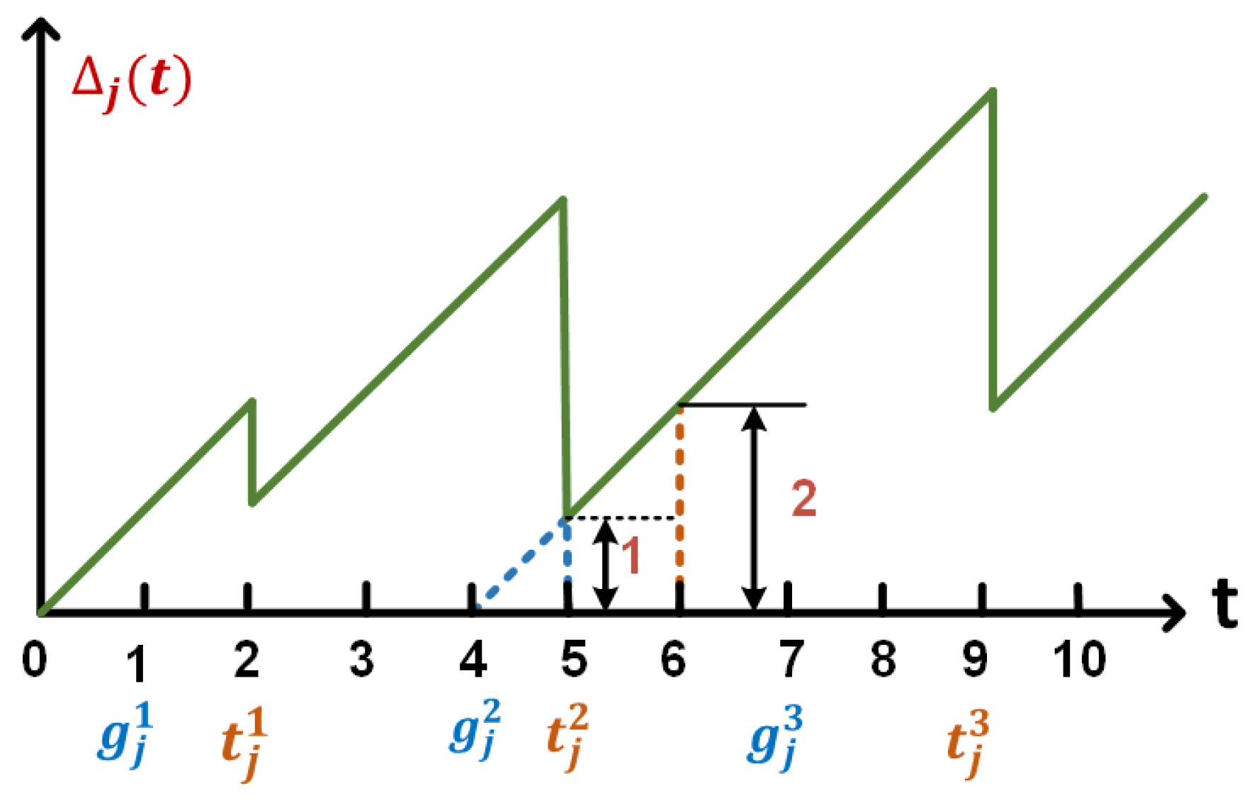Figure 3 depicts the AoI update process of the data generated by sensor node $j\in \mathcal{M}$. The set of data generation instants is denoted as $G_j=\{g_j^1,g_j^2,\dots ,g_j^{\phi },\dots \}$, where $g_j^{\phi }=(\phi -1)\times {\nu }_j+1$, $\phi$ is the index of data generated by sensor node j, and ${\nu }_j$ is the time period of sensing data generation for the sensor node j. $\{t_j^1,t_j^2,\dots \}$ is the set of the transmission instants for sensor node j. For example, for sensor node j, the data update period ${\nu }_j=3$, the first data generation time is $g_j^1=1$, and $g_j^{\phi }$ will update to $g_j^2={\nu }_j+1=4$ when the second sensing data are generated.

All data must be transmitted as soon as possible before new data are generated. Therefore, at time slot t, based on the uploading decision of sensor node j, the AoI for sensor node j will be updated as

$${\Delta }_j(t+1)=\left\{\begin{array}{c}{\Delta }_j(t)+1,{\alpha }_j(t)=0;\\ t-g_j^{\phi }+1,{\alpha }_j(t)=1.\end{array}\right.$$

(16)

As shown in Figure 3, at the time slot $t=4$, sensor node j generates its second sensing data (i.e., $g_j^2=4$), and it decides not to upload the newly generated data (i.e., ${\alpha }_j(t)=0$). The AoI for sensor node j increases linearly in this time slot since the BS does not receive new data updates from sensor node j. Therefore, the corresponding AoI will be updated to ${\Delta }_j(t)+1$ at the next time slot $t+1$. At the time slot $t=5$, sensor node j uploads the second sensing data with ${\alpha }_j(t)=1$. Thus, at the next time slot $t+1$, the corresponding AoI is updated to $t-g_j^{\phi }+1$, which is the time interval from the second data generation instant to the data upload instant plus 1 unit, where $g_j^{\phi }$ and t are the second data generation instant and transmission instant, respectively, $t_f=1$ unit is the time interval from the data transmission instant t to the time slot $t+1$, and $\phi =2$. Therefore at time slot $t=6$, the AoI is updated to 2.

3.5. Value Function of the Collected Data

For each task, when a sensor node generates new data, the old data become invalid if they are not collected by UAVs. In order to collect more valid data, tasks that need to be updated frequently are more urgent in data collection. At the same time, we aim to minimize the AoI of all tasks. Therefore, we define that the value of the collected data depends on two factors: ${\nu }_j$ and ${\Delta }_j(t)$, $j\in \mathcal{M}$.

For the sensing data of two tasks with the same update period, the smaller the AoI of the collected sensing data, the higher the value of the sensing data. Additionally, for a task, a smaller update period means that it is more urgent to collect the generated sensing data. Therefore, with the same AoI of the collected sensing data from different tasks, the shorter its update period ${\nu }_j$, the higher the value of the collected data. Based on the aforementioned features, we define the value of the collected data from sensor node j as

$$F_j(t)=\gamma (\frac{{\omega }_1}{{\nu }_j}+\frac{{\omega }_2}{{\Delta }_j(t)}),$$

(17)

where ${\omega }_1$ and ${\omega }_2$ are parameters used to balance data uploading decisions of sensor nodes with different update periods, for example, ${\omega }_1$ can be set to a high value when the update requirements of sensor nodes in the system are more urgent, and vice versa. $\gamma$ is a scaling parameter about the value of the collected data.

When ${\alpha }_j(t)=1$, sensor node j decides to upload sensing data to a UAV, the UAV needs to move to and hover above the sensor node j to collect the sensing data, and the energy consumption during the flight is related to the distance and speed of the flight. As a result, there is a trade-off between collecting more valid data and minimizing the energy consumption of the UAV.

4. Problem Formulation

Considering the value of all collected data and the energy consumption of all UAVs, we define the system utility function as the value of collected data minus the total energy consumption of all UAVs, which is described as

$$\begin{array}{c}\hfill \begin{array}{cc}\hfill U(t)=& \sum _{i\in \mathcal{N}}\sum _{c_k\in \mathcal{C}(t)}{\eta }_i^{c_k}(t)\sum _{j\in c_k}{\alpha }_j(t)\times F_j(t)-\sum _{i\in \mathcal{N}}\sum _{c_k\in \mathcal{C}(t)}{\eta }_i^{c_k}(t)[E_{i,1}(t)+E_{i,2}(t)\hfill \\ & +E_{i,3}(t)+E_{i,4}(t)]-\sum _{i\in \mathcal{N}}[1-\sum _{c_k\in \mathcal{C}(t)}{\eta }_i^{c_k}(t)]P_0\times t_f.\hfill \end{array}\end{array}$$

(18)

${\eta }_i^{c_k}(t)=1$ represents that UAV i is arranged to collect data from sensor nodes of cluster $c_k$ at time slot t. $c_k$ denotes one cluster which covers several sensor nodes. At each time slot t, the cluster set $\mathcal{C}(t)=\{c_1,c_2,\dots ,c_k,\dots \}$, $\forall c_k\in \mathcal{C}(t)$ is divided according to the upload decisions of sensor nodes, and the details are discussed in Section 4.2. When UAV i is not arranged to collect any sensing data (i.e., it will keep hovering at its current location), we have ${\sum }_{c_k\in C(t)}{\eta }_i^{c_k}(t)=0$.

Our objective is to maximize the system utility given in (18) while satisfying different data freshness requirements during the whole sensing period. There exists a trade-off between collecting more valuable data and consuming less energy. Therefore, we optimize the UAVs trajectories, the UAVs flight speeds, and the sensor nodes’ upload decisions with the constraints of diverse AoI requirements. We formulate the whole problem as follows:

$$\begin{array}{cc}\hfill \mathrm{P}1:& \hfill \underset{\alpha ,\eta ,l^{uav},v}{max}U(t)\hfill \end{array}$$

(19)

$$\begin{array}{cc}\hfill s.t.& {\tau }_{i,1}(t)+{\tau }_{i,2}(t)+{\tau }_{i,3}(t)+{\tau }_{i,4}(t)=t_f,\forall i\in \mathcal{N},\hfill \\ \hfill & {\alpha }_{i,j}(t)\in \{0,1\},\forall i\in \mathcal{N},\forall j\in \mathcal{M},\hfill \end{array}$$

(19a)

$$\begin{array}{cc}\hfill & \hfill {\alpha }_j(t)\in \{0,1\},\forall j\in \mathcal{M},\hfill \end{array}$$

(19b)

$$\begin{array}{cc}\hfill & \hfill \sum _{i\in \mathcal{N}}{\eta }_i^{c_k}(t)\in \{0,1\},\hfill \end{array}$$

(19c)

$$\begin{array}{cc}\hfill & \hfill \sum _{c_k\in \mathcal{C}(t)}{\eta }_i^{c_k}(t)\in \{0,1\},\hfill \end{array}$$

(19d)

$$\begin{array}{cc}\hfill & \hfill \underset{T\to \infty }{lim}\frac{1}{T}\sum _{t=0}^T{\Delta }_j(t)\le {\nu }_j,\forall j\in \mathcal{M},\hfill \\ \hfill & \hfill v_{min}\le v_{i,1}(t)\le v_{max},\forall i\in \mathcal{N},\hfill \end{array}$$

(19e)

$$\begin{array}{cc}\hfill & \hfill v_{min}\le v_{i,2}(t)\le v_{max},\forall i\in \mathcal{N}.\hfill \end{array}$$

(19f)

The constraint (19a) indicates that each UAV must perform the four stages within a time slot. At time slot t, the data upload decision ${\alpha }_j(t),\forall j\in \mathcal{M}$ and the UAV cluster-matching decision ${\eta }_i^{c_k}(t),\forall i\in \mathcal{N},\forall c_k\in \mathcal{C}(t)$ are integer variables in (19b–19d). Sensor node j can only upload data to one UAV at a time, denoted as ${\alpha }_j(t)={\sum }_{i\in \mathcal{N}}{\alpha }_{i,j}(t)\le 1$. In case UAV i is arranged to collect data from sensor node j, it is denoted as ${\alpha }_{i,j}(t)=1$; otherwise, ${\alpha }_{i,j}(t)=0$. Therefore, we need to optimize the location of UAVs and try to avoid overlapping coverage of UAVs. The time to collect data ${\tau }_{i,2}(t)$, the time to transmit data ${\tau }_{i,4}(t)$, the movement time ${\tau }_{i,1}(t)$ and ${\tau }_{i,3}(t)$ are non-integer variables no less than zero as are $v_{i,1}(t)$ and $v_{i,2}(t)$, the flying velocities of UAV i. The speeds of UAVs during the two movement stages cannot exceed the limit in (19f). In order to maintain the freshness of the information, the average AoI cannot exceed the update period of each sensor node as in (19e). The flight speed and flight trajectory require optimal decision making at each time slot. The optimization problem $\mathrm{P}1$ becomes complicated and intractable when all these variables are coupled at each time slot.

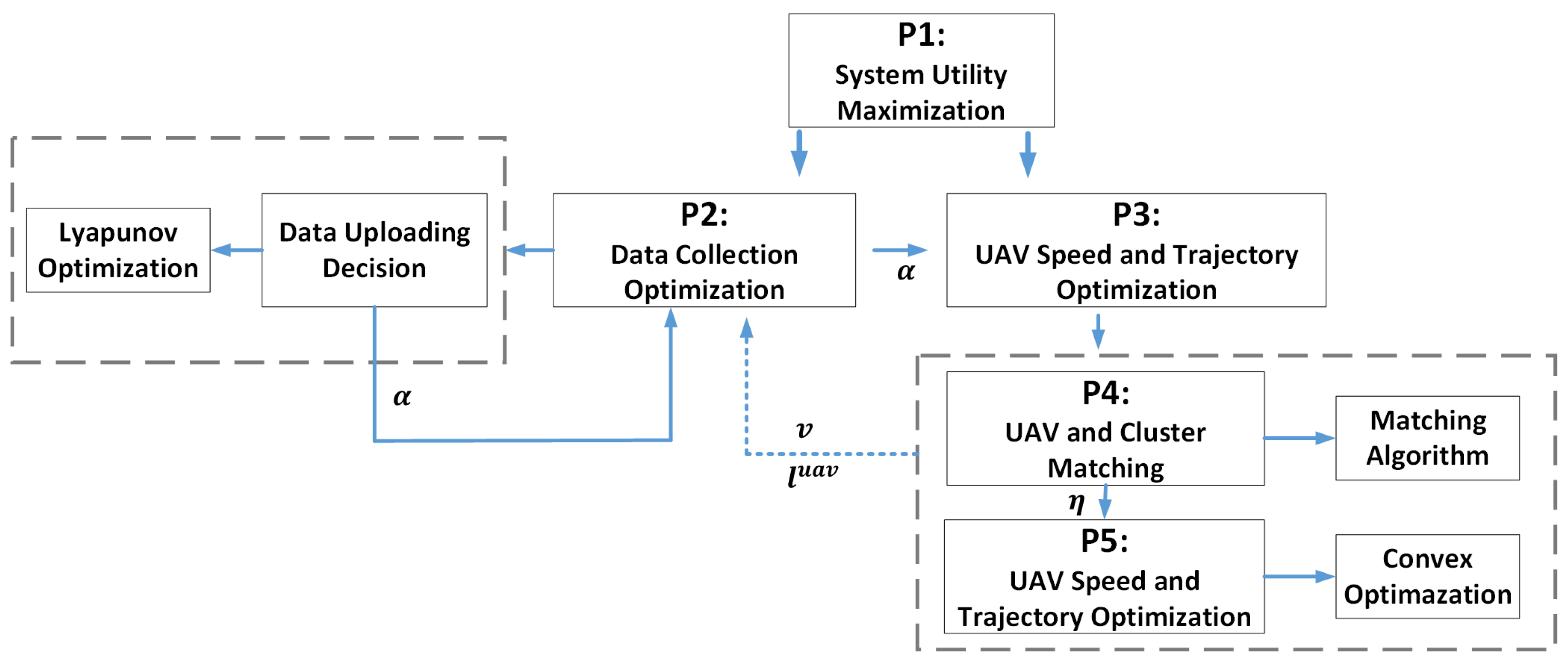
Therefore, we decompose problem $\mathrm{P}1$ into two sub-problems $\mathrm{P}2$ and $\mathrm{P}3$. As shown in Figure 4, in problem $\mathrm{P}2$, we solve the upload decision of sensor nodes given the initial location and flight speed of UAVs. Then, we determine the flight trajectory and flight speed of UAVs in problem $\mathrm{P}3$, according to the obtained uploading decision of sensor nodes:

$$\begin{array}{cc}\hfill \mathrm{P}2:& \hfill \underset{\alpha }{max}U(t)\hfill \\ \hfill s.t.& \hfill (19\mathrm{b},19\mathrm{e}).\hfill \end{array}$$

(20)

$$\begin{array}{cc}\hfill \mathrm{P}3:& \underset{\eta ,l^{uav},v}{max}U(t)\hfill \\ \hfill s.t.& (19\mathrm{a},19\mathrm{c},19\mathrm{d},19\mathrm{f}).\hfill \end{array}$$

(21)

Problem $\mathrm{P}3$ is also difficult to solve directly since the variables are complicated. We then decouple problem $\mathrm{P}3$ into two sub-problems $\mathrm{P}4$ and $\mathrm{P}5$. $\mathrm{P}4$ is to determine the first stop location of UAVs and the matching outcome $\eta$ while maximizing system utility; the matching algorithm is used to solve this problem. Then we solve the UAVs speed $v_1,v_2$ and the second stop location in problem $\mathrm{P}5$, which is a convex optimization problem. At last, we perform $\mathrm{P}2$ and $\mathrm{P}3$ iteratively to obtain the solution.

4.1. Data Collection Optimization

The data collection optimization problem $\mathrm{P}2$ is to solve the uploading decision of sensor nodes as follows:

$$\begin{array}{cc}\hfill \mathrm{P}2:& \hfill \underset{\alpha }{max}U(t)\hfill \\ \hfill s.t.& \hfill (19\mathrm{b},19\mathrm{e}).\hfill \end{array}$$

(22)

With distinct requirements for data freshness, each sensor node updates its sensing data with a different update period. To ensure the relative freshness of different types of information, the average AoI must not exceed the update period of sensing data for each sensor node, which is the time-average constraint given in (19e). To address this, we employ Lyapunov optimization [30] and first construct the dynamic virtual queue $Q_j(t)$, representing the relative update period increment of the AoI for sensor node j at time slot t:

$$Q_j(t+1)=max\{Q_j(t)+{\Delta }_j(t)-{\nu }_j,0\},$$

(23)

where ${\Delta }_j(t)$ is the AoI for sensor node j at time slot t, and ${\nu }_j$ is the time interval between successive data generated at sensor node j. The larger the difference between them, the lower the freshness of the collected data.

Then, we construct the Lyapunov function denoted as $L(t)=\frac{1}{2}Q{(t)}^2$. In order to keep the virtual queue $Q(t)$ rate stable at each time slot, the Lyapunov drift [30] should be minimized as follows:

$$\begin{array}{cc}\hfill min\Delta L(t)& =\frac{1}{2}\sum _{j\in \mathcal{M}}[Q_j{(t+1)}^2-Q_j{(t)}^2]\hfill \\ \hfill & =\frac{1}{2}\sum _{j\in \mathcal{M}}[max{\{Q_j(t)+{\Delta }_j(t)-{\nu }_j,0\}}^2-Q_j{(t)}^2]\hfill \\ \hfill & =\frac{1}{2}\sum _{j\in \mathcal{M}}[max{\{Q_j(t)+(1-{\alpha }_j(t))({\Delta }_j(t)+1)+{\alpha }_j(t)(t-g_j^{\phi }+1)-{\nu }_j,0\}}^2-Q_j{(t)}^2].\hfill \end{array}$$

(24)

Our objective is to maximize system utility while ensuring the average AoI constraint in (19e). As the flight speed and the stop location of UAVs are known, we can calculate the energy consumption during the two movement stages of UAVs. Consequently, we only need to focus on energy consumption during the stages of data collection and data transmission. Therefore, at each time slot, our aim is to minimize the Lyapunov drift minus the system utility [30], which can be expressed as follows:

$$\begin{array}{cc}\hfill & \Delta L(t)-\chi \sum _{j\in \mathcal{M}}{\alpha }_j(t)[F_j(t)-P_0\frac{L_j}{R_i^j(t)}-P_i(t)\frac{L_j}{R_{uav,i}^{bs}(t)}]\hfill \\ \hfill & \le W+\sum _{j\in \mathcal{M}}[Q_j(t)+{\Delta }_j(t)+1-{\nu }_j][t-g_j^{\phi }-{\Delta }_j(t)]{\alpha }_j(t)\hfill \\ \hfill & +\chi [P_0\sum _{j\in \mathcal{M}}\frac{L_j}{R_i^j(t)}+\sum _{j\in \mathcal{M}}{P}_i(t)\frac{L_j}{R_{uav,i}^{bs}(t)}-F_j(t)]{\alpha }_j(t).\hfill \end{array}$$

(25)

$\chi$ is a control parameter for a trade-off between the queue length of the AoI relative increment and the system utility. W is a constant. We assume that UAV i collects data from sensor node j at time slot t.

Theorem 1.

At time slot t, given UAV i’s stop location and flight speed, namely $l_{i,1}^{uav}(t),l_{i,2}^{uav}(t)$, $v_{i,1}(t)$, and $v_{i,2}(t)$, the optimal uploading decision ${\alpha }_j(t)$ is given as

$$\begin{array}{cc}\hfill & \hfill {\alpha }_j(t)=\left\{\begin{array}{cc}1,& Q_j(t)\le \chi [F_j(t)-P_0\frac{L_j}{R_i^j(t)}-P_i(t)\frac{L_j}{R_{uav,i}^{bs}(t)}]{(t-g_j^{\phi }-{\Delta }_j(t))}^{-1}-{\Delta }_j(t)-1+{\nu }_j;\\ 0,& else.\end{array}\right.\hfill \end{array}$$

(26)

Proof of Theorem 1.

To minimize the drift minus utility, we need to find the upper bound of the right side of inequality (25). If the virtual queue length $Q_j(t)$ is no more than $\chi [F_j(t)-P_0\frac{L_j}{R_i^j(t)}-P_i(t)\frac{L_j}{R_{uav,i}^{bs}(t)}]{(t-g_j^{\phi }-{\Delta }_j(t))}^{-1}-{\Delta }_j(t)-1+{\nu }_j$, this means the relative AoI increment of sensor node j is larger, and the urgency of the next data update of sensor node j is much higher. Otherwise, ${\alpha }_j(t)=0$.    □

4.2. UAV and Cluster Matching Problem

After all sensor nodes decide whether to upload data at time slot t, we cluster all sensor nodes with ${\alpha }_j(t)=1$ using the K-means clustering method [31]. This divides all sensor nodes with ${\alpha }_j(t)=1$ into several clusters. The cluster set is denoted as $\mathcal{C}(t)=\{c_1,c_2,\dots ,c_k,\dots \}$, where each $c_k\in \mathcal{C}(t)$ includes several sensor nodes. At each time slot, the sensing data from sensor nodes in one cluster are collected by one UAV. Problem $\mathrm{P}4$ aims to solve the arrangement of the first stop location of UAVs to efficiently collect the sensing data for different clusters:

$$\begin{array}{cc}\hfill & \hfill \mathrm{P}4:\underset{\eta }{max}U(t)\hfill \\ \hfill & \hfill s.t.(19\mathrm{c},19\mathrm{d}).\hfill \end{array}$$

(27)

Since the decision of each sensor node is determined, the problem of maximizing the system utility can be transformed into the problem of minimizing energy consumption. That is, the problem $\mathrm{P}4$ is equivalent to the following problem:

$$\begin{array}{cc}\hfill \underset{\eta }{min}& E(t)=\sum _{i\in \mathcal{N}}{\eta }_i^{c_k}(t)[E_{i,1}(t)+E_{i,2}(t)+E_{i,3}(t)+E_{i,4}(t)]-\sum _{i\in \mathcal{N}}[1-\sum _{c_k\in \mathcal{C}(t)}{\eta }_i^{c_k}(t)]P_0\times t_f\hfill \\ \hfill & s.t.(19\mathrm{c},19\mathrm{d}).\hfill \end{array}$$

(28)

We apply a one-to-one matching algorithm [32] to solve this problem. With a set of clusters composed of different sensor nodes and a set of UAVs $\mathcal{N}$, our objective is to decide the outcome of the one-to-one matching between the set of clusters and the set of UAVs, denoted as the matching pair set $\kappa =\{(i,c_k),\dots \},i\in \mathcal{N},c_k\in \mathcal{C}(t)$.

The one-to-one matching of UAVs and clusters is the result of the first stopping locations of UAVs. UAV i will match with, at most, one of the clusters at each time slot, or fail to match, which means that UAV i keeps hovering at its location in this time slot. If UAV i does not match any cluster, the matching pair is denoted as $(i,c_0)$, where $c_0$ denotes the unmatched state of each UAV. Cluster $c_k$ will also match, at most, one UAV, or fail to match, which means that no UAV will go over to cluster $c_k$ to collect data at this time slot, corresponding to constraint (19c,19d).

Let $V_i(c_k)$ denotes the utility function of UAV i and the cluster $c_k$, which is given as

$$\begin{array}{cc}\hfill V_i(c_k)=& {\eta }_i^{c_k}(t)[E_{i,1}(t)+E_{i,2}(t)+E_{i,3}(t)+E_{i,4}(t)]+[1-{\eta }_i^{c_k}(t)]P_0\times t_f,\hfill \\ \hfill & \forall c_k\in \mathcal{C}(t),\forall i\in \mathcal{N}.\hfill \end{array}$$

(29)

According to the utility function, at each time slot, each UAV can choose one cluster that is most willing to match or stay in place, and the cluster can find the most preferred UAV to pair with. Algorithm 1 gives the detailed process to solve $\eta (t)$ and matching pair set $\kappa$. At the beginning, we compute the utility of all UAVs and clusters. Next, for each $i\in \mathcal{N}$, we find the UAV i’s preferred cluster $c_k$ from the set ${\mathcal{C}}^{†}(t)$ based on (29); ${\mathcal{C}}^{†}(t)$ is equivalent to the cluster set $\mathcal{C}(t)$. Then, for the cluster $c_k$, when it is successfully matched with UAV i, UAV i will move to cluster $c_k$ for data collection at time slot t, and ${\eta }_i^{c_k}(t)=1$. Then we remove UAV i from the set $\mathcal{N}$ and remove $c_k$ from $\mathcal{C}(t)$. If cluster $c_k$ is not successfully matched with UAV i, we will delete cluster $c_k$ from the set ${\mathcal{C}}^{†}(t)$; UAV i continues to match with the other clusters in the set ${\mathcal{C}}^{†}(t)$ until this set is empty. UAVs that are not successfully matched will stay in place.

Algorithm 1 UAV cluster-matching algorithm

1: Compute the utility of all UAVs and clusters based on (29);   2: Matching pair set $\kappa \leftarrow \varnothing ,{\eta }_i^{c_k}(t)=0,\forall i\in \mathcal{N},\forall c_k\in \mathcal{C}(t)$;   3: for each UAV $i\in \mathcal{N}$ do   4:     ${\mathcal{C}}^{†}(t)=\mathcal{C}(t)$   5:     while ${\mathcal{C}}^{†}(t)\ne \varnothing$ do   6:        $c_k=argmax\{V_i(c_k),c_k\in {\mathcal{C}}^{†}(t)\}$;   7:        $\rho =argmax\{V_i(c_k),i\in \mathcal{N}\}$;   8:        if $\rho =i$ then   9:           ${\eta }_i^{c_k}(t)=1,\kappa \leftarrow (i,c_k)$; 10:           Delete $c_k$ from $\mathcal{C}(t)$, Delete i from $\mathcal{N}$; 11:           break; 12:        else 13:            Delete $c_k$ from $\mathcal{C}†(t)$, 14:         end if 15:      end while 16: end for 17: return   Matching pair set $\kappa$ and $\eta (t)$.

4.3. UAV Trajectory and Speed Optimization

At time slot t, we obtain the upload decision $\alpha (t)$ for sensor nodes and the matching variable $\eta (t)$ for UAVs and sensor clusters. With these determined parameters, the flight speed and flight trajectory of UAVs at each time slot can be solved in the problem $\mathrm{P}5$:

$$\begin{array}{cc}\hfill & \hfill \mathrm{P}5:\underset{l^{uav},v}{max}U(t)\hfill \\ \hfill & \hfill s.t.(19\mathrm{a},19\mathrm{f}).\hfill \end{array}$$

(30)

Since the uploaded decision and matching variable are already determined, we transform the objective function of problem $\mathrm{P}5$ into minimizing the energy consumption of UAVs with four stages:

$$\begin{array}{cc}\hfill \underset{l^{uav},v}{min}{E}_2(t)=\hfill & \sum _{i\in \mathcal{N}}\sum _{c_k\in \mathcal{C}(t)}{\eta }_i^{c_k}(t)[E_{i,1}(t)+E_{i,2}(t)+E_{i,3}(t)+E_{i,4}(t)]\hfill \\ \hfill s.t.\hfill & (19\mathrm{a},19\mathrm{f}).\hfill \end{array}$$

(31)

It can be proved that the function $E_2(t)$ is a convex function [33] and the variables $v_1$ and $v_2$ can be solved with the CVX solver. The energy consumption function $E_2(v_{i,1},v_{i,2})$ of UAV i is expressed as follows:

$$\begin{array}{cc}\hfill & E_2(v_{i,1},v_{i,2})=E_{i,1}(t)+E_{i,2}(t)+E_{i,3}(t)+E_{i,4}(t)\hfill \\ \hfill =& [s_1(1+\frac{3{(v_{i,1}(t))}^2}{{(v_{tip})}^2})+s_2{(\sqrt{1+\frac{{(v_{i,1}(t))}^4}{4{(v_0)}^4}}-\frac{{(v_{i,1}(t))}^2}{2{(v_0)}^2})}^{\frac{1}{2}}+\frac{1}{2}{s}_3{(v_{i,1}(t))}^3]·{\tau }_{i,1}(t)+P_0\times {\tau }_{i,2}(t)\hfill \\ \hfill & +P_i\times {\tau }_{i,4}(t)+[s_1(1+\frac{3{(v_{i,2}(t))}^2}{{(v_{tip})}^2})+s_2{(\sqrt{1+\frac{{(v_{i,2}(t))}^4}{4{(v_0)}^4}}-\frac{{(v_{i,2}(t))}^2}{2{(v_0)}^2})}^{\frac{1}{2}}+\frac{1}{2}{s}_3{(v_{i,2}(t))}^3]·{\tau }_{i,3}(t)\hfill \\ \hfill & s.t.{\tau }_{i,1}(t)+{\tau }_{i,2}(t)+{\tau }_{i,3}(t)+{\tau }_{i,4}(t)=t_f,\hfill \\ \hfill & v_{min}\le v_{i,1}(t)\le v_{max},\hfill \\ \hfill & v_{min}\le v_{i,2}(t)\le v_{max}.\hfill \end{array}$$

(32)

Since ${\tau }_{i,2}(t)$ and ${\tau }_{i,4}(t)$ are determined, $E_2(v_{i,1},v_{i,2})$ is the function with respect to variables $v_{i,1}$ and $v_{i,2}$.

Theorem 2.

The function $E_2(v_{i,1},v_{i,2})$ is a convex function with respect to $v_{i,1},v_{i,2}$.

Proof of Theorem 2.

$$\begin{array}{cc}\hfill & \frac{\partial E_2}{\partial v_{i,1}}=3\frac{s_1}{{(v_{tip})}^2}+s_3{v}_{i,1}+\frac{s_2{(v_{i,1})}^2}{{[(\sqrt{1+\frac{{(v_{i,1})}^4}{4{(v_0)}^4}}-\frac{{(v_{i,1})}^2}{2{(v_0)}^2})(1+\frac{{(v_{i,1})}^4}{4{(v_0)}^4})]}^{\frac{1}{2}}4{(v_0)}^4}\hfill \\ \hfill & -\frac{s_2}{{(\sqrt{1+\frac{{(v_{i,1})}^4}{4{(v_0)}^4}}-\frac{{(v_{i,1})}^2}{2{(v_0)}^2})}^{\frac{1}{2}}2{(v_0)}^2}-\frac{s_2{(\sqrt{1+\frac{{(v_{i,1})}^4}{4{(v_0)}^4}}-\frac{{(v_{i,1})}^2}{2{(v_0)}^2})}^{\frac{1}{2}}+s_1}{{(v_{i,1})}^2}.\hfill \end{array}$$

(33)

$$\begin{array}{cc}\hfill & \frac{{\partial }^2}{\partial v_{i,1}\partial v_{i,1}}{E}_2=s_3+\frac{s_2}{2{(v_0)}^4{[(\sqrt{1+\frac{{(v_{i,1})}^4}{4{(v_0)}^4}}-\frac{{(v_{i,1})}^2}{2{(v_0)}^2})(1+\frac{{(v_{i,1})}^4}{4{(v_0)}^4})]}^{\frac{1}{2}}}\hfill \\ \hfill & +\frac{s_2{(v_{i,1})}^3}{8{(v_0)}^8{(\sqrt{1+\frac{{(v_{i,1})}^4}{4{(v_0)}^4}}-\frac{{(v_{i,1})}^2}{2{(v_0)}^2})}^{\frac{1}{2}}{(1+\frac{{(v_{i,1})}^4}{4{(v_0)}^4})}^{\frac{3}{2}}}\frac{s_2}{{(\sqrt{1+\frac{{(v_{i,1})}^4}{4{(v_0)}^4}}-\frac{{(v_{i,1})}^2}{2{(v_0)}^2})}^{\frac{1}{2}}}[\frac{{(v_{i,1})}^3}{4{(v_0)}^4{(1+\frac{{(v_{i,1})}^4}{4{(v_0)}^4})}^{\frac{1}{2}}}\hfill \\ \hfill & -\frac{1}{2{(v_0)}^2}][\frac{1}{2{(v_0)}^2}-\frac{{(v_{i,1})}^2}{4{(v_0)}^4{(1+\frac{{(v_{i,1})}^4}{4{(v_0)}^4})}^{\frac{1}{2}}}-\frac{1}{{(v_{i,1})}^2}]+\frac{2s_2{(\sqrt{1+\frac{{(v_{i,1})}^4}{4{(v_0)}^4}}-\frac{{(v_{i,1})}^2}{2{(v_0)}^2})}^{\frac{1}{2}}}{{(v_{i,1})}^3}+\frac{2s_1}{{(v_{i,1})}^3}.\hfill \end{array}$$

(34)

$$\frac{{\partial }^2}{\partial v_{i,1}\partial v_{i,2}}{E}_2=0,\frac{{\partial }^2}{\partial v_{i,2}\partial v_{i,1}}{E}_2=0.$$

(35)

The energy consumption function $E_2(v_{i,1},v_{i,2})$ of UAV i is a function with respect to two variables $v_{i,1}$ and $v_{i,2}$ with the range $[v_{min},v_{max}]$. The function $E_2(v_{i,1},v_{i,2})$ has continuous second derivatives on the definition domain, and $\frac{{\partial }^2}{\partial v_{i,2}\partial v_{i,2}}{E}_2$ gives the similar result as in (34).

The second-order partial derivative matrix of the function $E_2$ is denoted as follows [33]:

$$H=\left[\begin{array}{cc}\frac{{\partial }^2}{\partial v_{i,1}\partial v_{i,1}}{E}_2& \frac{{\partial }^2}{\partial v_{i,1}\partial v_{i,2}}{E}_2\\ \frac{{\partial }^2}{\partial v_{i,2}\partial v_{i,1}}{E}_2& \frac{{\partial }^2}{\partial v_{i,2}\partial v_{i,2}}{E}_2\end{array}\right]\ge 0.$$

(36)

For $(v_{i,1},v_{i,2})$ and $(v_{o,1},v_{o,2})$, $\forall i,o\in \mathcal{N}$, and $0\le \theta \le 1$, the following inequality is held [33]:

$$E_2(\theta v_{i,1}+(1-\theta )v_{o,1},\theta v_{i,2}+(1-\theta )v_{o,2})\le \theta E_2(v_{i,1},v_{i,2})+(1-\theta )E_2(v_{o,1},v_{o,2}).$$

(37)

   □

The first-order derivative of the function $E_2$ exists and is continuous, and the second-order derivative exists and is semi-positive definite. We demonstrate that the problem $\mathrm{P}5$ is a convex optimization problem. Therefore, the flight speeds $v_{i,1},v_{i,2}$ of UAV i can be solved by convex optimization. The second stopping location $l_{i,2}^{uav}$ of UAV i can be determined by the flight speeds $v_{i,1},v_{i,2}$ and movement time ${\tau }_{i,1},{\tau }_{i,3}$ of UAV i.

4.4. Iteration Algorithm

We propose the Algorithm 2 to solve the upload decision $\alpha (t)$ of the sensor nodes, the trajectories $l_1^{uav}(t),l_2^{uav}(t)$, and the flight speeds $v_1(t),v_2(t)$ of UAVs at time slot t. For the first iteration with $n=1$, the problem $\mathrm{P}1$ is decoupled into two sub-problems: $\mathrm{P}2$ and $\mathrm{P}3$. In $\mathrm{P}2$, we know the initial flight speeds $v_1^0$ and $v_2^0$ of UAVs, which allows us to solve the uploading strategy ${\alpha }^1$. Efficient data upload decision for sensor nodes with different update requirements can be achieved using Lyapunov optimization while ensuring the relative AoI for each task.

Algorithm 2 Optimal diversified demands algorithm (ODDA)

1: Input: $Q(t),\Delta (t)$   2: Output: $l_1^{uav}(t),l_2^{uav}(t),U(t)$;   3: Initialize $v_1^0,v_2^0$, $E^0$, $l_1^{uav,0},l_2^{uav,0}$;   4: $n=1$;   5: while$\left|E^n-E^{n-1}\right|\ge ϵ$ and $n\le n^{max}$ do   6:    Determine the uploading decision ${\alpha }^n$ by Lyapunov optimization;   7:    Determine the clusters $C^n$ for all sensor nodes with ${\alpha }^n=1$;   8:    Perform Algorithm 1 to obtain the matching pair set $\kappa$ and the first stop location $l_1^{uav,n}$ of UAVs;   9:    Perform convex optimization to obtain flight speed $v_1^n,v_2^n$ and the second stop location $l_2^{uav,n}$ of UAVs; 10:    Compute the energy consumption $E^n$ with (28); 11:    $n=n+1$; 12: end while 13:    Update the AoI $\Delta (t+1)$ with (16); 14: Update the queue $Q(t+1)$ with (23); 15: Compute the system utility $U(t)$ with (18).

Next, we further decouple the problem $\mathrm{P}3$ into problem $\mathrm{P}4$ and problem $\mathrm{P}5$. Based on the determined upload decision ${\alpha }^n$, all sensor nodes with ${\alpha }^n=1$ are clustered, and each cluster may serve as the first stop location of UAVs in $\mathrm{P}4$. Notably, each UAV can cover at most one cluster, and sensor nodes in each cluster can upload data to, at most, one UAV. Therefore, by using a one-to-one matching algorithm, we can determine the first stop locations $l^{uav,n}1$ of UAVs. Subsequently, with the first stop locations of UAVs, the value of the collected data, and the time consumed to upload the data to UAVs, we can transform problem $\mathrm{P}5$ into a convex optimization problem aiming to minimize the energy consumption of UAVs. Solving this convex optimization problem yields the flight speeds $v_1^n$ and $v_2^n$, as well as the second stopping locations of UAVs $l^{uav,n}2$.

The first iteration is then completed, and we proceed with subsequent iterations until the difference in energy consumption $E^n$ of UAVs between two consecutive iterations is less than the given threshold $ϵ$, or the number of iterations exceeds the maximum specified number of iterations $n^{max}$. At that point, the iteration terminates, and we move on to the next time slot $t+1$.

5. Performance Evaluation

In this section, we present simulation results to demonstrate the performance of our proposed method ODDA. We consider a UAV-assisted sensing data collection system that consists of one BS, N UAVs, and M sensor nodes. The sensor nodes are randomly distributed in a rectangular area with a length of 20 km and a width of 15 km. The whole sensing time is divided into $T=1000$ time slots. Other parameters are listed in

Table 2. Simulation parameter.

Designation	Notation	Value
The maximal UAV flight velocity	$v_{max}$	20 m/s
The minimal UAV flight velocity	$v_{min}$	5 m/s
The UAV flight height	H	50 m
Time duration of each time slot	$t_f$	150 s
Transmission power of UAV i	$P_i$	0.1 watt
Carrier frequency	$f_c$	2 GHz
Noise power	${\sigma }^2$	$-110$ dBm
The speed of light	c	$3\times {10}^8$ m/s
The channel gain at $d_0=1$ m	${\beta }_0$	$-60$ dB
Average additional loss of LoS link	${\mu }_{los}$	1 dB
Average additional loss of NLoS link	${\mu }_{nlos}$	10 dB
Environment constants	$a,b$	$10, 0.3$
System bandwidth allocate to UAV i	$B_i$	10 MHz
The data packet length	L	1 Mbits
Data update period of sensor nodes	$\nu$	1∼8

.

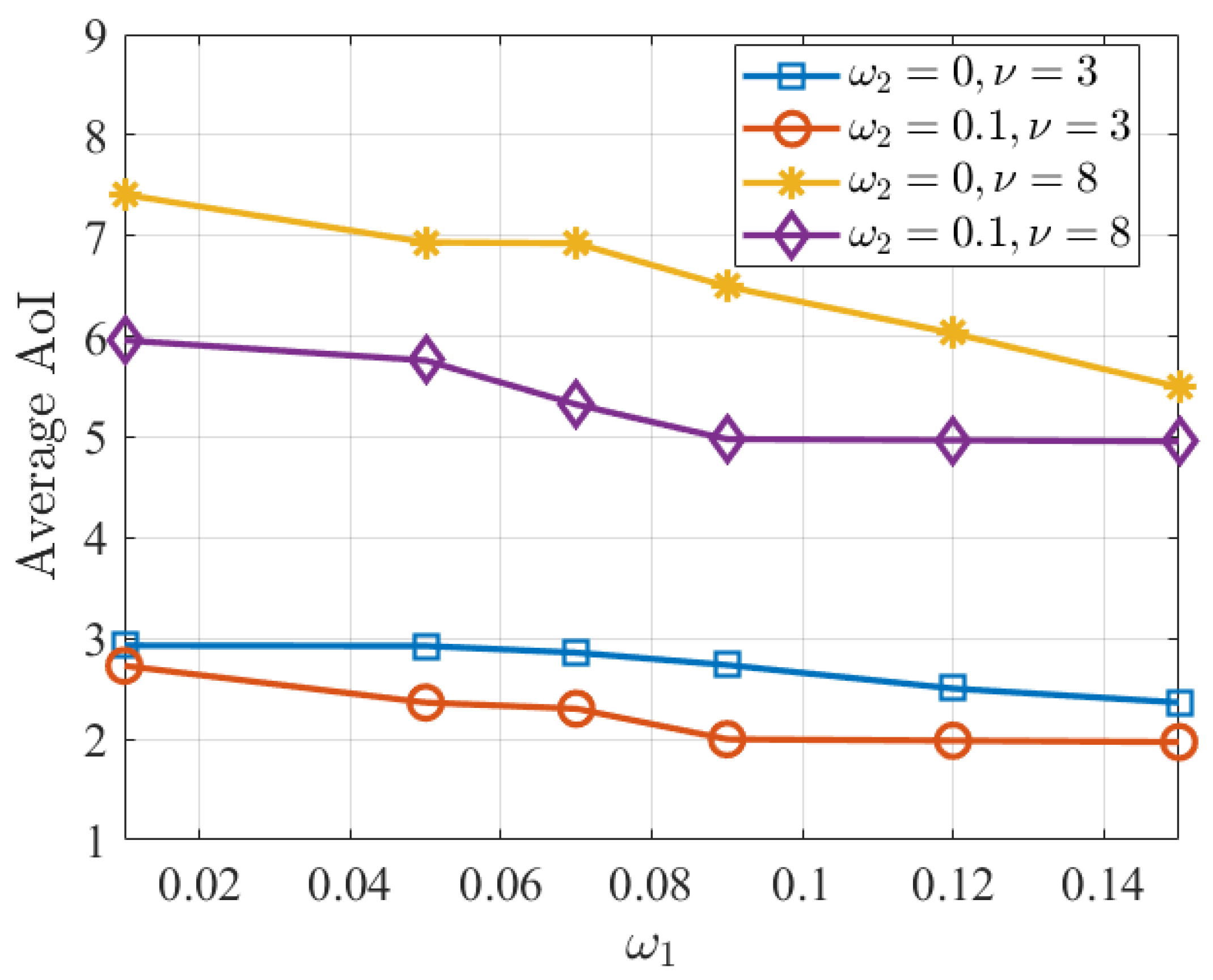
Figure 5 depicts the average AoI versus different weights ${\omega }_1$, where the number of UAVs and the sensor nodes are set as $N=2$ and $M=10$, respectively. Each of the ten sensor nodes has a data update period of either 3 or 8. $\nu =3$ represents the sensor node that requires a higher frequency of information updates, and $\nu =8$ represents the sensor node that requires a lesser frequency of updates. It is observed that with the increase in ${\omega }_1$, the shorter average AoI can be achieved. We define the average AoI as the ratio of the sum of the information ages of the corresponding sensor nodes to the total time slot T. Meanwhile, the average AoI for sensor nodes with short update periods (e.g., $\nu =3$) is smaller than the average AoI for sensor nodes with long update periods (e.g., $\nu =8$) since we consider the relative AoI for sensor nodes with different update periods, rather than blindly minimizing the age of all information. With the same value of ${\omega }_1$, the average AoI of the sensor node gradually decreases as the weight ${\omega }_2$ increases for sensor nodes with $\nu =3$ or $\nu =8$. Meanwhile, it is also observed that ${\omega }_1$ has more significant impacts on the sensor node with a shorter data update period (e.g., $\nu =3$).

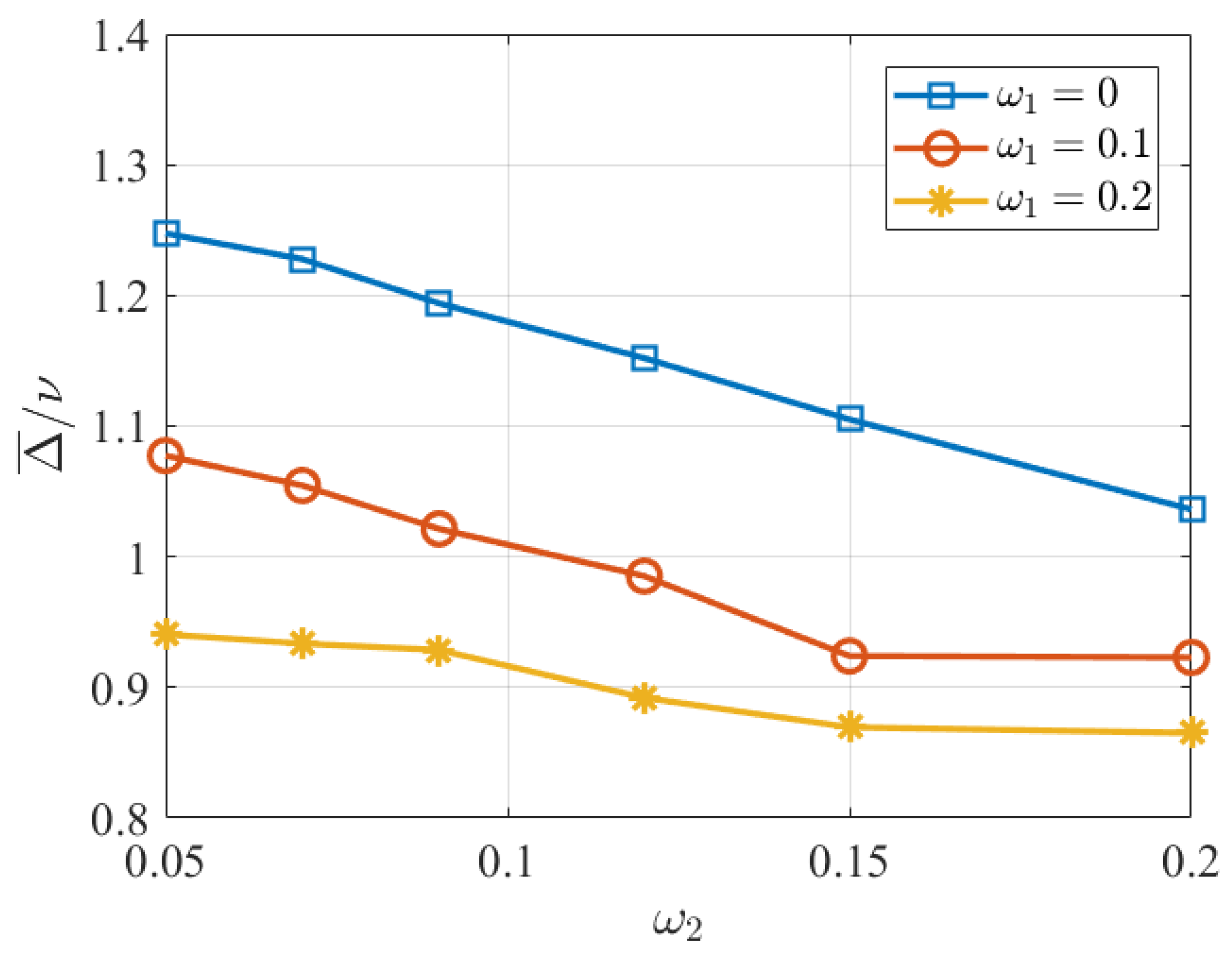
To further demonstrate the achieved AoI with respect to the corresponding sensing data update period, we define the relative AoI as the ratio of the achieved average AoI to the update period of the corresponding sensing data denoted as $\overline{\Delta }/\nu$. Figure 6 depicts $\overline{\Delta }/\nu$ for sensor nodes with $\nu =3$ versus different values of the weight ${\omega }_2$ for different sets of the weight ${\omega }_1$. It is observed that the relative AoI decreases with the increase in ${\omega }_2$. In addition, with the same value of ${\omega }_2$, the relative AoI decreases with increases in ${\omega }_1$. This is because increasing ${\omega }_1$ enhances the importance of sensor nodes with a short update period, resulting in faster data collection and consequently lower relative AoI for sensor nodes with an update period $\nu =3$.

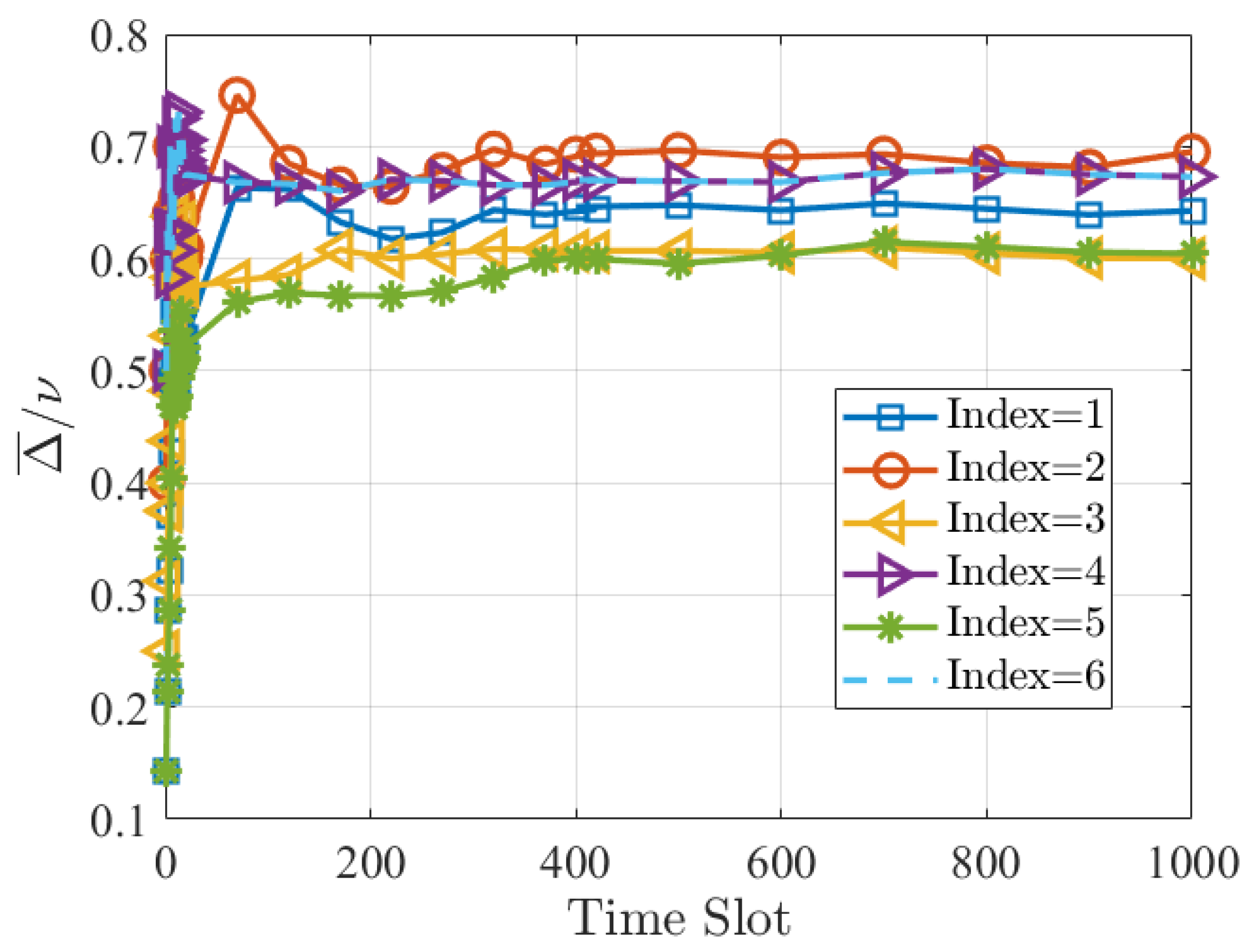
Figure 7 shows the convergence of relative AoI for sensor nodes with different update periods. We set the update periods for six sensor nodes as $\nu \in \{2,3,4,5,6,8\}$, indicating that the AoI requirements vary across sensor nodes. It is observed that the relative AoI gradually converges to a constant value. It is also observed that the relative AoI $\overline{\Delta }/\nu$ for each sensor node is less than 1, demonstrating that our proposed method ensures the relative freshness of information from sensor nodes with various update periods.

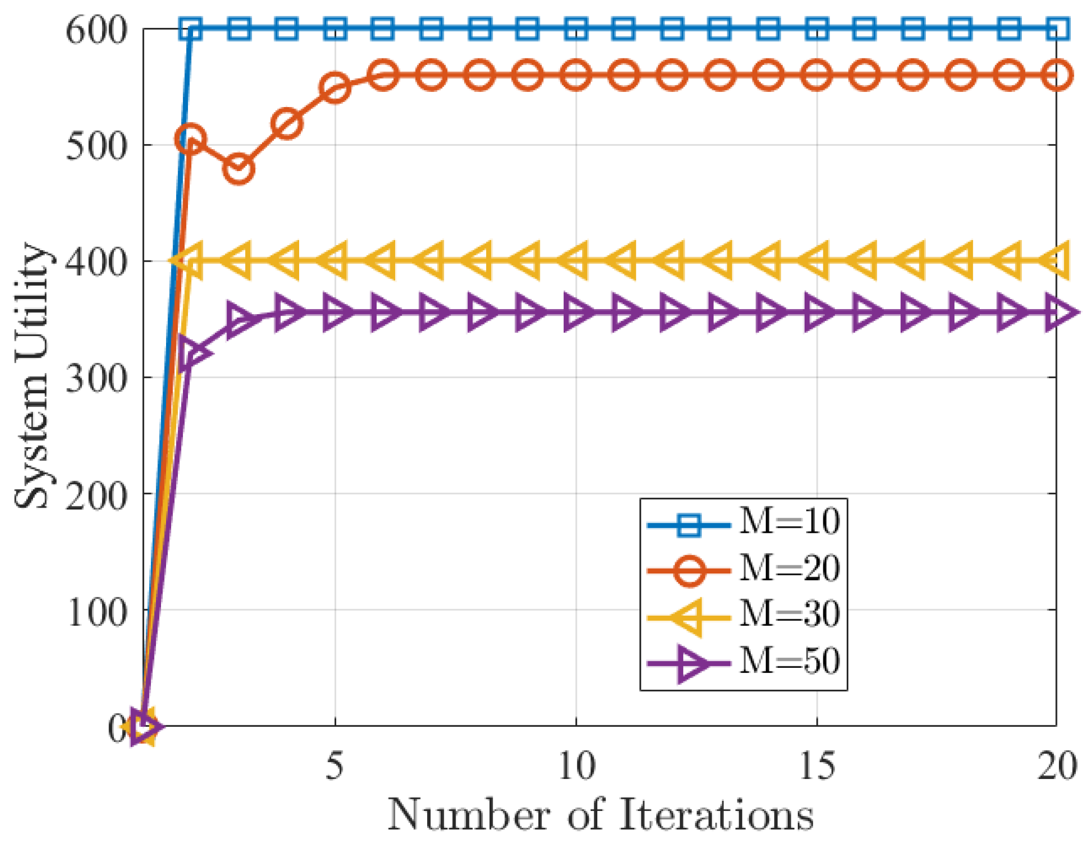
Figure 8 demonstrates the algorithm convergence with different settings of M (i.e., the number of sensor nodes). It is observed that the system utility can quickly converge to a stable value in different settings.

We then compare the performance of our proposed method with the following four methods:

(1)

Age optimal algorithm (AOA): Based on our proposed method, at each time slot t, we consider a strategy in that sensing data are collected as early as possible after their generation, aiming to minimize the AoI of all sensor nodes without considering the diversity of sensor nodes’ update periods. In computing $F(t)$, we omit the effect of ${\omega }_1$. Other parameters are set in the same way as in our method.

(2)

Diverse requirement optimal algorithm (DROA): Based on our proposed method, at each time slot t, we consider a strategy that only focuses on the diversity of sensor nodes’ update periods. It does not take into account the overall system’s AoI. The effect of weight ${\omega }_2$ is omitted. Other parameters are set in the same way as in our method.

(3)

Energy minimizing algorithm (EMA): Based on our proposed method, at each time slot t, we consider a strategy that focuses on minimizing the energy consumption of UAVs. It disregards the overall system’s AoI and the diversity of sensor nodes’ update periods. We do not consider the effect of data values. The effects of ${\omega }_1$ and ${\omega }_2$ are ignored. The objective function is to minimize energy consumption. The other parameters are set in the same way as in our method.

(4)

DRL-eFresh [8]: DRL-eFresh guarantees data freshness by setting a deadline in each time slot, aiming to maximize the collected data amount and geographical fairness without considering the diversity of the sensor nodes’ update periods.

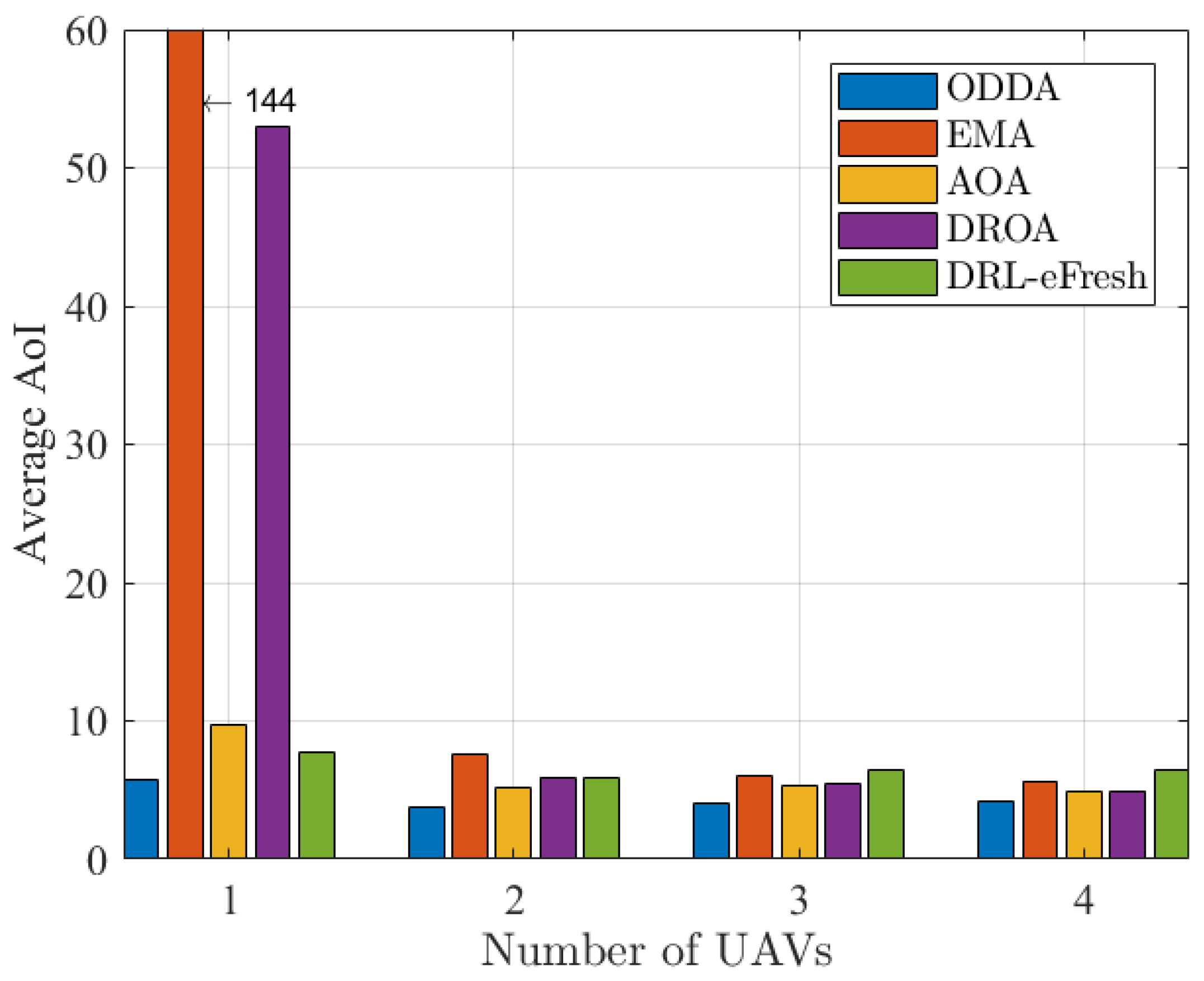
Figure 9 depicts the average AoI versus different numbers of UAVs, where the number of sensor nodes is set as $M=10$. The number of sensor nodes is set to 10, which assumes that when the number of UAVs is 4, it is possible for all UAVs to cover all sensor nodes through scheduling. It is observed that our proposed method ODDA can achieve a shorter average AoI compared with the other four methods. EMA focuses solely on minimizing energy consumption, disregarding the timeliness of information. DROA only considers the urgency of different types of data to ensure timeliness by prioritizing frequently updated data while neglecting the less frequently updated data. It is observed that DROA and EMA perform much worse than our proposed ODDA, AOA, and DRL-eFresh when the number of UAVs is 1. AOA aims to reduce the age of all information but overlooks the varying urgency levels of different types of sensing data. DRL-eFresh focuses on the collected data amount and geographical fairness but neglects the different levels of data urgency requirements. With the increase in the number of UAVs, the average AoI reduces due to the increased flexibility of the UAVs’ operation, which allows for more dynamic and efficient data collection.

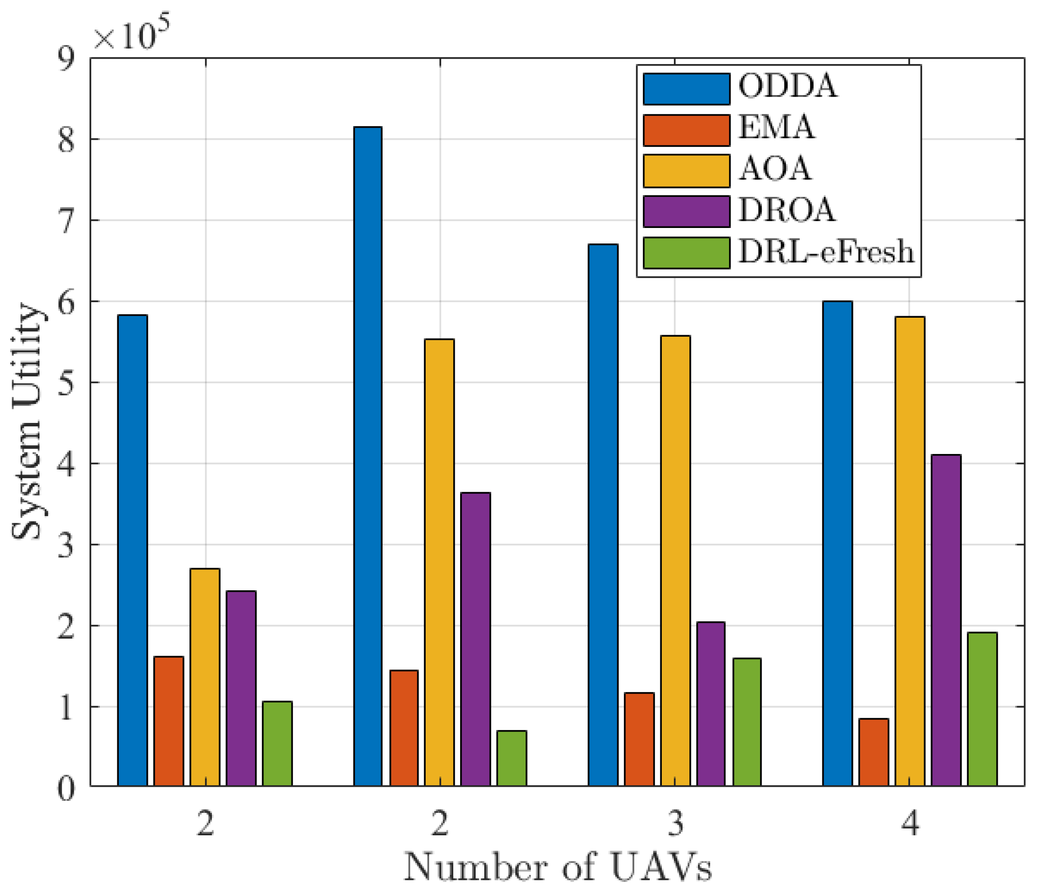
Figure 10 depicts the achieved system utility versus different numbers of UAVs. It is observed that our proposed method ODDA outperforms the other four methods. Specifically, our proposed method can improve the system utility by $714\%$, $47\%$, $124\%$, and $1088\%$ with the setting of 2 UAVs compared to EMA, AOA, DROA, and DRL-eFresh, respectively. It is also observed the system utility with our proposed method increases at first, then decreases with the increasing numbers of UAVs. The change in the number of UAVs will have impacts on both the number of data collected and the energy consumption of UAVs. On the one hand, increasing the number of UAVs leads to an increase in the amount of collected sensing data, which can positively impact the system’s utility. On the other hand, increasing the number of UAVs results in an increase in the energy consumption of UAVs. In the beginning, the positive impacts outweigh the negative impacts of the increasing energy consumption, leading to an increase in the achieved system utility. Gradually, however, the increase in energy consumption starts to outweigh the benefits of collecting more data. Consequently, the system utility tends to decrease. Thus, employing a larger number of UAVs may not be the most efficient approach in terms of system utility performance.

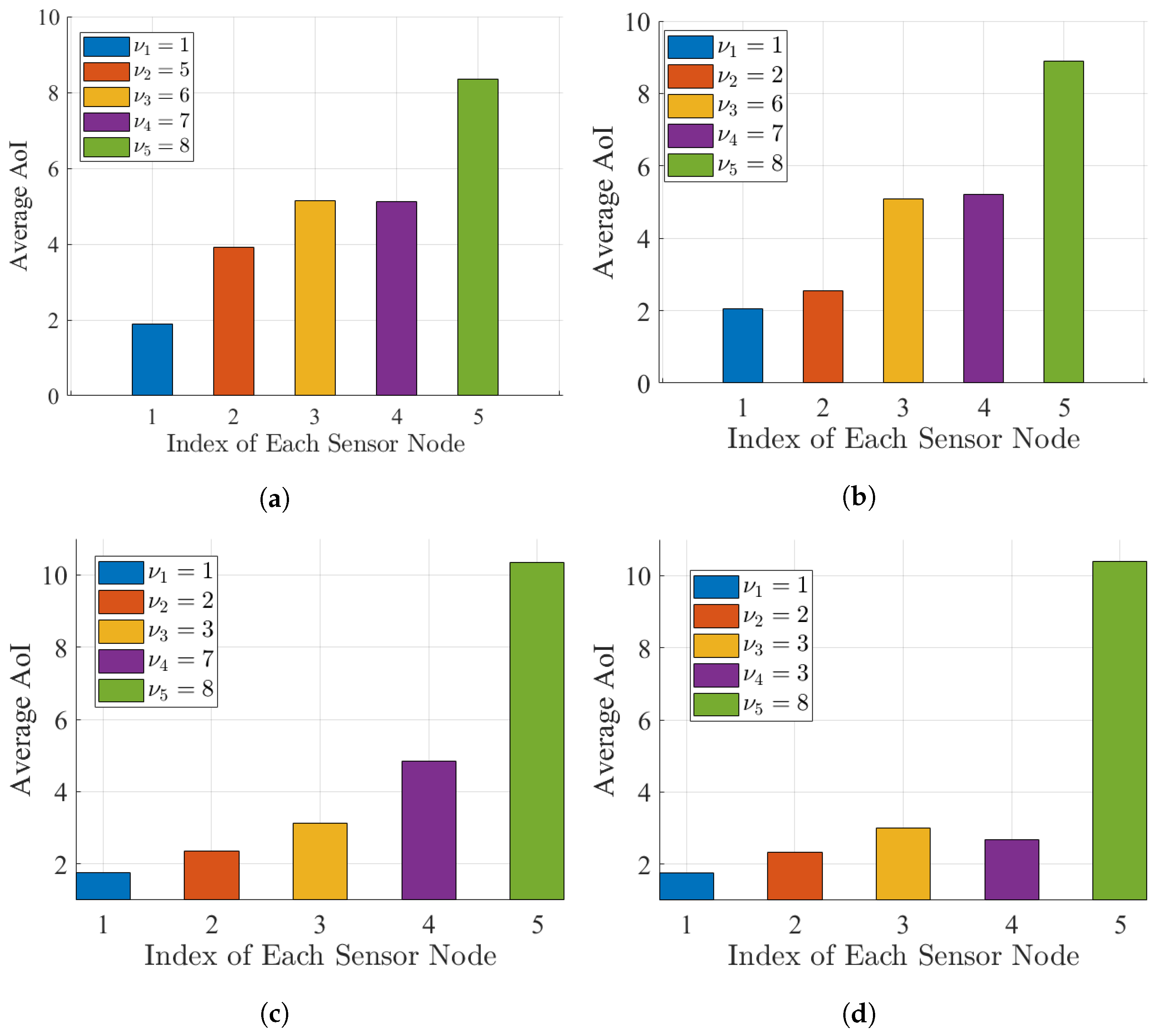
In different application scenarios, the requirements for data freshness can vary. In Figure 11, we consider four scenarios with different percentages of urgent sensing data: $\{20\%,40\%,60\%,80\%\}$, where we set the data update period for urgent demand as $\nu \in \{1,2,3\}$ and the number of sensor nodes as $M=5$, and ${\nu }_j,j\in \{1,2,3,4,5\}$ denotes the data update period of sensor node j. It can be observed in Figure 11 that the average AoI increases with the increase in the sensor node’s update period. Specifically, the first sensor node with the most urgent update period achieves the shortest AoI, while the 5th sensor node with the longest update period obtains the longest AoI. This is due to the consideration of the relative freshness of sensor nodes at different update periods. As the percentage of urgent data increases, the average AoI for the sensor node with a large update period (e.g., ${\nu }_5=8$) also increases. This is because higher priority is put on the urgent data.

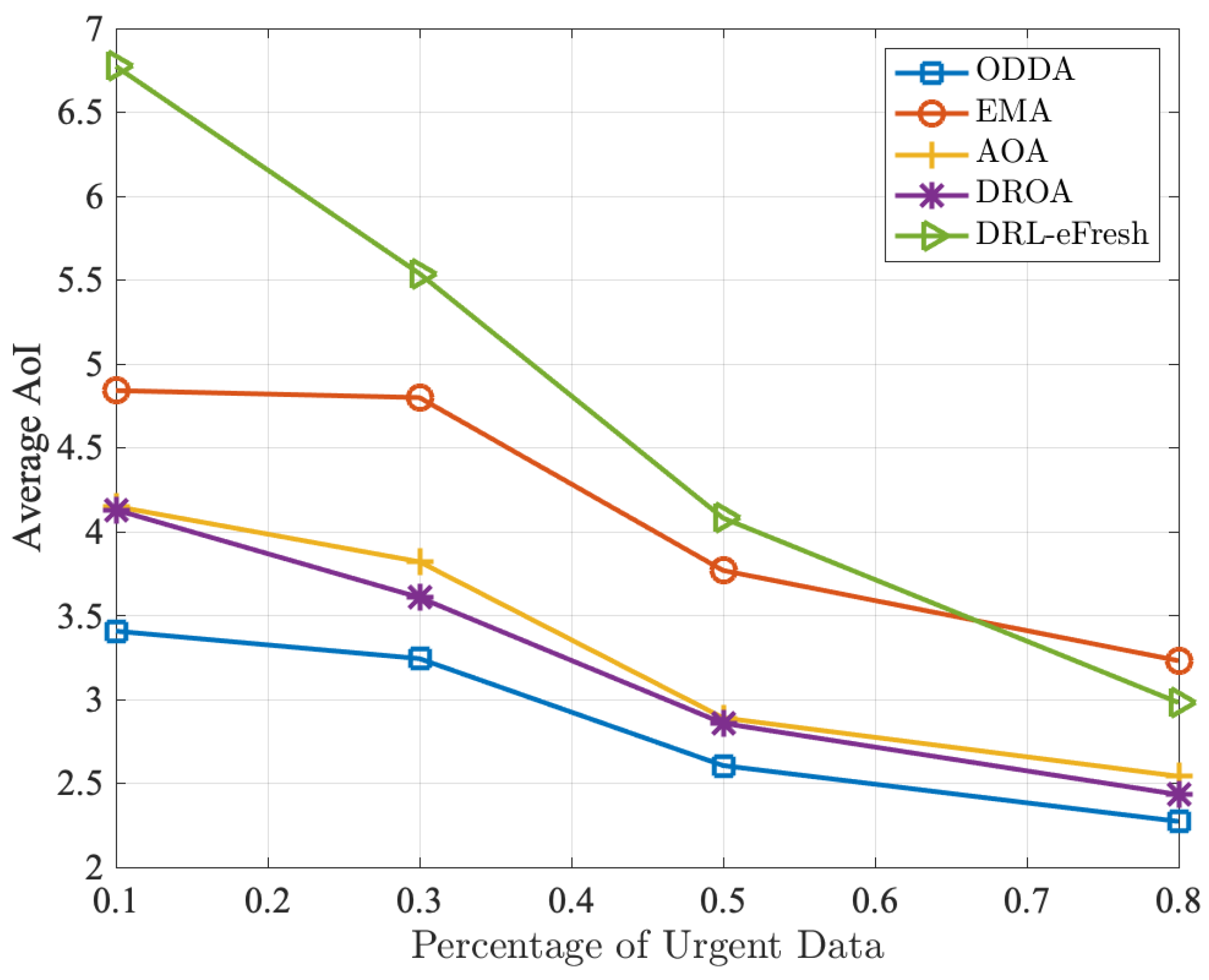
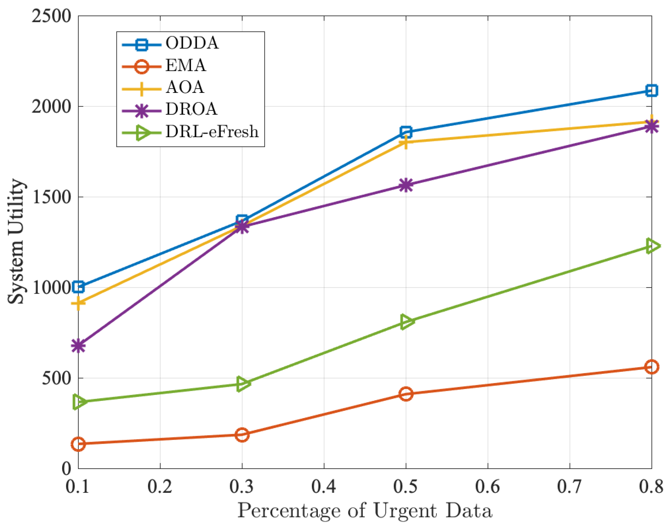
Figure 12 and Figure 13 depict the average AoI and system utility versus the percentage of data with urgent requirements, respectively. It is observed that our method ODDA can achieve the smallest average AoI among the five methods. As the percentage of sensing data with urgent update requirements increases, more sensor nodes update their sensing data faster, leading to a higher frequency of collecting sensing data. Consequently, the average AoI decreases, and the system utility increases.

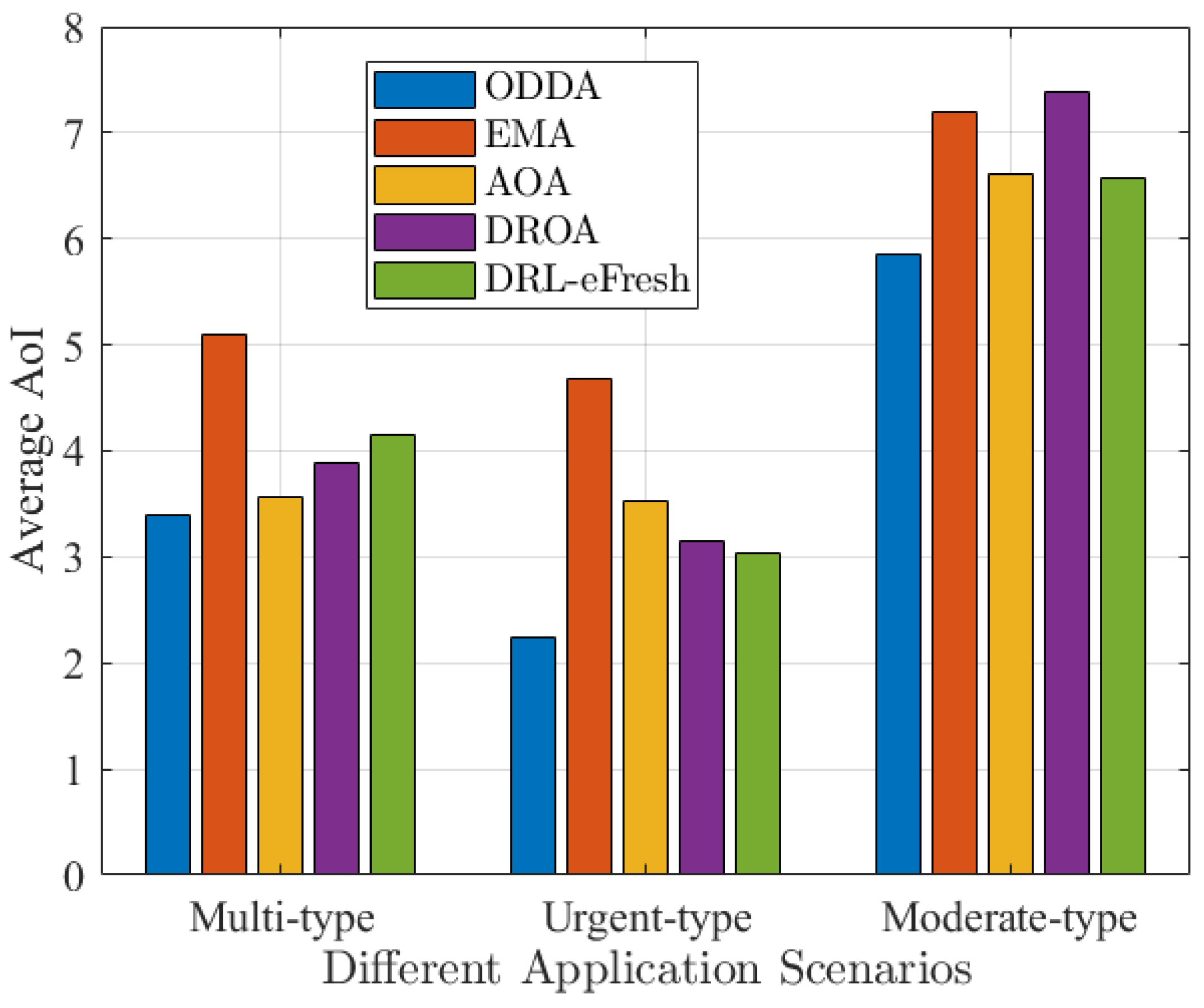
Figure 14 shows the average AoI with three scenarios (denoted as multi-type, urgent type, and moderate type). In the smart city, the multi-type scenario includes diverse types of sensor nodes with the update periods ranging from $\nu \in [1,8]$. The urgent-type scenario emphasizes relatively urgent update requirements, with the update periods for all sensor nodes set in the range of $\nu \in [1,3]$. For example, traffic monitoring and public safety require real-time data collection for timely decision making and response to emergencies. In the moderate-type scenario, the update periods of all sensor nodes are relatively lenient, with the update periods set in the range of $\nu \in [6,8]$. Applications such as environmental monitoring, for example, where data can be updated less frequently, can follow a certain cycle of data collection. It is observed that our proposed method ODDA outperforms the other four counterparts in all three scenarios. Specifically, in the urgent-type scenario, our method can achieve average AoI reductions of $56\%$, $40\%$, $34\%$, and $26\%$ compared to EMA, AOA, DROA, and DRL-eFresh, respectively. It is also observed that the achieved average AoI is the smallest in the urgent-type scenario and the largest in the moderate-type scenario. More sensor nodes update their sensing data faster in the urgent-type scenario, leading to a higher frequency of collecting sensing data.

Our method employs an efficient data collection strategy to meet various information updating requirements. By monitoring the data update period and timeliness requirements of different tasks, we can flexibly adjust the task execution order and path planning of UAVs in each time slot based on the urgency and priority of different tasks. For tasks with relatively urgent update requirements, UAVs can be prioritized for data collection and transmission to ensure timely data transmission. On the other hand, for tasks with lenient update requirements, data collection can be scheduled for subsequent time periods, thereby reducing system energy consumption and improving overall efficiency.

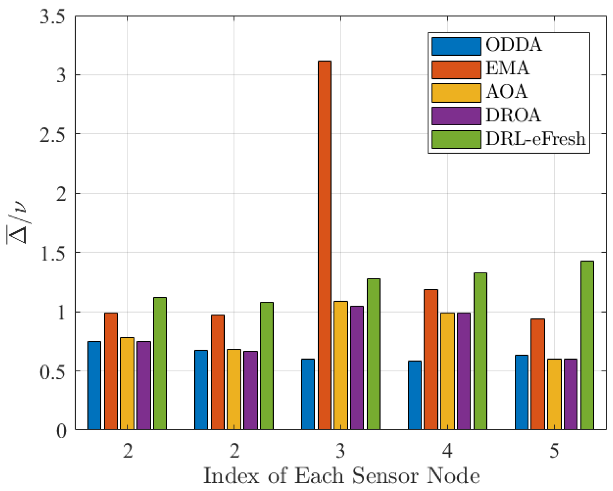
Figure 15 illustrates the relative AoI for sensor nodes with different update periods, where the update periods of sensor nodes 1 to 5 are set as 2, 3, 5, 6, and 7, respectively. The result clearly demonstrates the superior performance of our method compared to the other four methods in terms of the relative AoI of each sensor node. Our method ensures that the relative information freshness $\overline{\Delta }/\nu$ of each sensor node remains below 1, rather than simply minimizing the overall AoI for the system. This highlights its ability to outperform other methods for tasks with different update requirements.

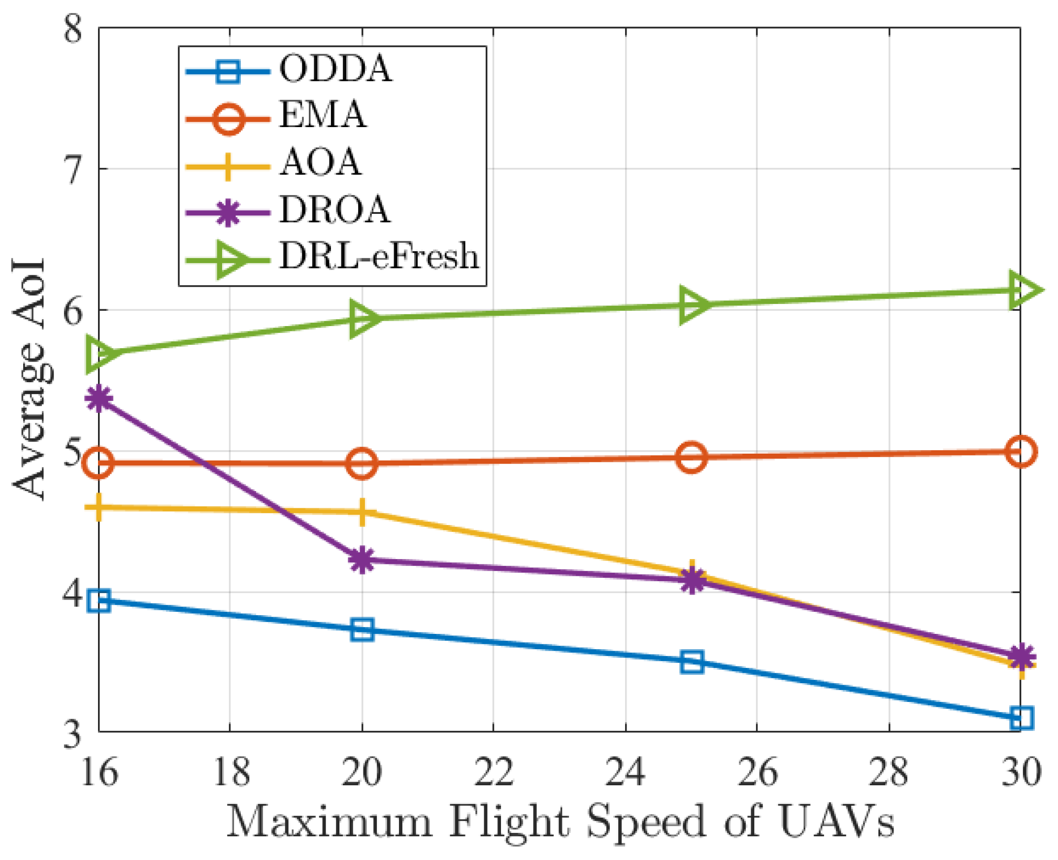
Figure 16 shows the average AoI versus the maximum flight speeds of UAVs, where the maximum flight speeds of UAVs are set as $v_{max}\in \{16,20,25,30\}$. Evidently, our proposed method ODDA outperforms the other four methods. By increasing the maximum UAV flight speed and implementing a scheduling strategy that optimizes data collection, more data can be efficiently collected, resulting in a notable decrease in the average AoI.

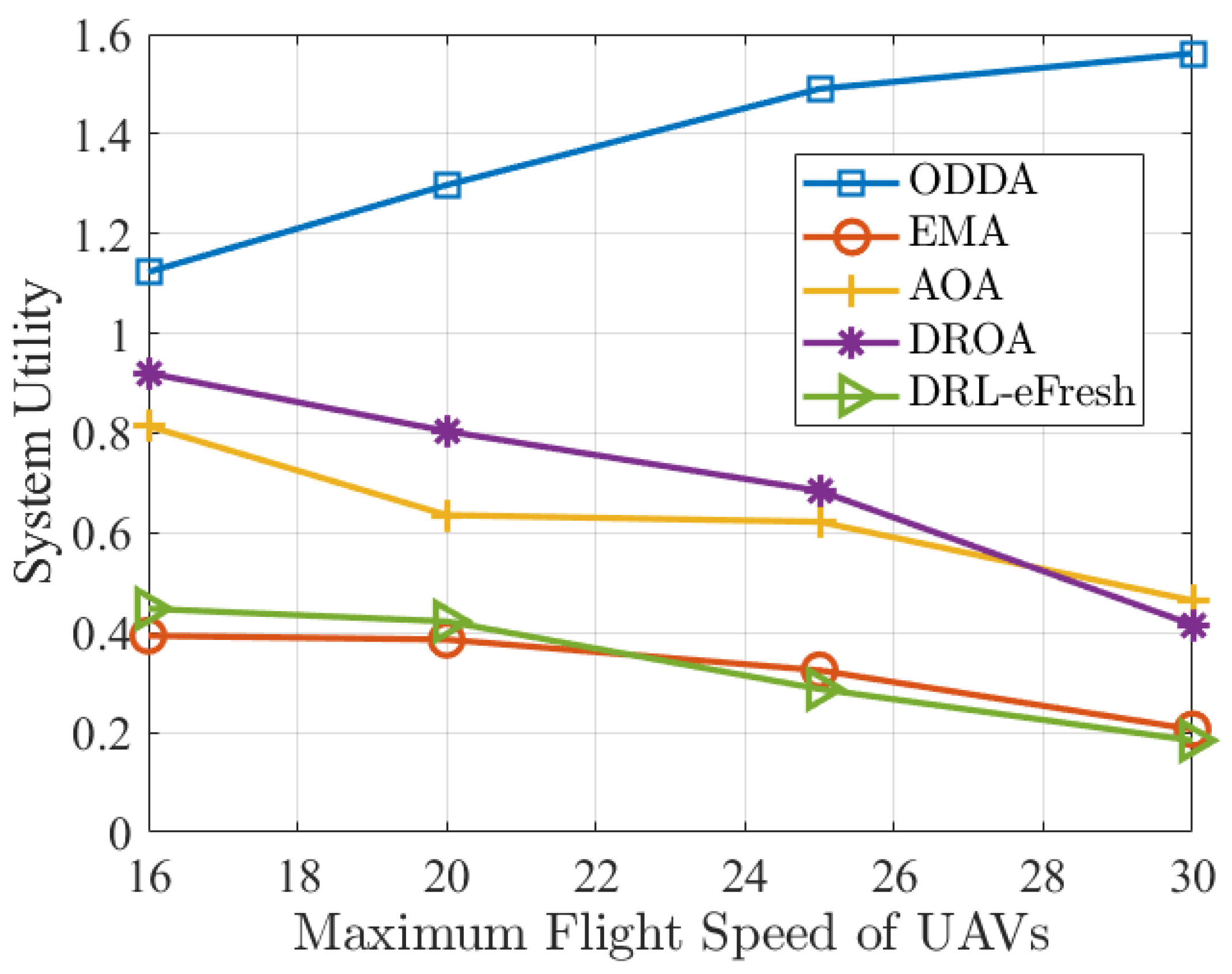
Figure 17 shows the system utility versus the maximum flight speeds of UAVs. It is observed that our proposed method ODDA outperforms the other four methods. The maximum UAV flight speed is increased, and our method enables us to optimize both the data collection scheduling and UAV flight speed, resulting in an enhanced system utility. However, the system utility of the other four methods diminishes with rising maximum flight speeds, as higher UAV energy consumption leads to reduced system utility.

6. Conclusions

In this paper, we consider both the diversity of different tasks in terms of the data update periods and the AoI of the collected sensing information in the UAV-assisted sensing data collection system. We propose an efficient data collection method that takes advantage of the high flexibility and low cost of the deployment of UAVs to maximize the system utility while ensuring the freshness of the collected information relative to their respective update periods. Then, we propose an algorithm to solve the proposed optimization problem and optimize the data upload strategy of sensor nodes, and the hovering locations and flight speeds of UAVs.

The simulation results demonstrate that the proposed method outperforms the other four counterparts in terms of the achieved average AoI when the number of UAVs is 1. And our method outperforms the other four methods in terms of the relative AoI for sensor nodes with different update periods.